Bloch Oscillations in the Chains of Artificial Atoms Dressed with Photons

School of Electrical Engineering, Tel Aviv University, Tel Aviv 39040, Israel
*
Author to whom correspondence should be addressed.
Appl. Sci. 2018, 8(6), 937; https://doi.org/10.3390/app8060937
Submission received: 28 April 2018
/
Revised: 31 May 2018
/
Accepted: 2 June 2018
/
Published: 6 June 2018
(This article belongs to the Special Issue Nano-Antennas)
Abstract
:We present a model of one-dimensional chain of two-level artificial atoms driven with DC field and quantum light simultaneously in a strong coupling regime. The interaction of atoms with light leads to electron-photon entanglement (dressing of the atoms with light). The driving via dc field leads to the Bloch oscillations (BO) in the chain of dressed atoms. We consider the mutual influence of dressing and BO and show that scenario of oscillations dramatically differs from predicted by the Jaynes-Cummings and Bloch-Zener models. We study the evolution of the population inversion, tunneling current, photon probability distribution, mean number of photons, and photon number variance, and show the influence of BO on the quantum-statistical characteristics of light. For example, the collapse-revivals picture and vacuum Rabi-oscillations are strongly modulated with Bloch frequency. As a result, quantum properties of light and degree of electron-photon entanglement become controllable via adiabatic dc field turning. On the other hand, the low-frequency tunneling current depends on the quantum light statistics (in particular, for coherent initial state it is modulated accordingly the collapse-revivals picture). The developed model is universal with respect to the physical origin of artificial atom and frequency range of atom-light interaction. The model is adapted to the 2D-heterostructures (THz frequencies), semiconductor quantum dots (optical range), and Josephson junctions (microwaves). The data for numerical simulations are taken from recently published experiments. The obtained results open a new way in quantum state engineering and nano-photonic spectroscopy.
1. Introduction
The early quantum theory of electrical conductivity in crystal lattices by Bloch, Zener and Wannier [1,2,3,4] led to the prediction that a homogeneous dc field induces an oscillatory rather than uniform motion of the electrons. These so-called Bloch oscillations (BO) have been observed in bulk N-doped GaAs at a lattice temperature of 300 K in high fields up to 300 kV/cm [5], as well as different types of artificial systems such as semiconductor superlattices [6], interacting atoms in optical lattices [7,8], ultracold atoms [9,10,11,12,13,14], light intensity oscillations in waveguide arrays [15,16,17,18,19,20,21], acoustic waves in layered and elastic structures [22], and atomic oscillations in Bose-Einstein condensates [23] among others. Several recent studies have investigated the dynamics of cold atoms in optical lattices subject to ac forcing; the theoretically predicted renormalization of the tunneling amplitudes has been verified experimentally. The recent observations include global motion of the atom cloud, such as giant “super-Bloch oscillations” [24]. As a result, BO transformed from the specific contra intuitive model to the general experimentally-supported physical concept of oscillatory motion of wave packets placed in a periodic potential when driven by a constant force [8,25].
Rabi oscillations (RO) are periodical transitions of a two-level quantum system between its stationary states under the action of an AC driving field [26,27]. The phenomenon was theoretically predicted by Rabi for the nuclear spins in radio-frequency magnetic field [28] and afterwards, discovered in various physical systems, such as electromagnetically driven individual atoms [29] including the case of Rydberg atomic states [30], semiconductor quantum dots (QDs) [31] and different types of solid-state qubits (superconducting charge qubits based on Josephson junctions [32,33,34], spin qubits [35], semiconductor charge qubits [36]). The textbook picture of the Rabi effect is given by the Jaynes-Cummings model [26,27]. It implied that the concept of the dressed atom with light was correspondent to the quantum entanglement of electrons and photons. This model can be essentially modified by a set of additional features, such as the broken inversion symmetry [37], the propagation of RO over the chains of coupled atoms in the form of special waves (Rabi-waves), and depolarization due to the local fields [38,39,40,41,42,43]. It opens the possibility of the generation of a variety of entangled quantum states, which could have a great impact on the search for universal and efficient quantum computation processes [44], the electrically tunable optical nano-antennas with highly directive emission [39,40,43], quantum sensing [45], and metrology [46]. Recent theoretical progress in this area is associated, in particular, with the novelty of inter-atomic coupling mechanisms [47,48], which manifests themselves in surprising thermodynamic behavior of the specific waveguiding arrays, which recently was experimentally verified [49].
In this paper, we build a theoretical model of a chain of coupled two-level quantum elements exposed to quantum light and driven via bias voltage. We consider the case of strong coupling of light with charge carriers, which lead to the entanglement of electron-photon quantum states. This model describes BO of electrons dressed with light and their mutual influence with RO. Our model has a significant degree of generality: It relates to the systems of different physical origin and various frequency ranges. We consider its application to semiconductor heterostructures (THz frequencies), semiconductor quantum dots (visible frequencies), and Josephson junctions (microwaves). For brevity, we refer to every of these artificial two-level quantum objects as an “atom” regardless of its physical implementation.
We develop the model taking into account conditions of real experiments. For example, the coherent inter-sub-band excitation of heterostructure in THz region has been done by the ultrashort (femtosecond) pulses [50]. On this account, we generalized our model for the case of electromagnetic pulse, advancing the secondary quantization of fields to the case of pulses. Our model is based on some conventional simplifications. We use rotating-wave approximation (RWA) and neglect any damping. This requires the fulfillment of certain relations between the frequencies (transmission frequency, light frequency, Rabi frequency, and Bloch frequency) and between some characteristic times (coherence time and attenuation time). Our calculations have been made for real physical parameters of atoms and their environment, and accessibility of these relations have been supported by the achievements of modern technologies and the data of published experiments. It allows the design of installations for potential future experiments in this branch.
The classical analog of our investigation is Rabi-Bloch oscillations (RBO) predicted in [51,52]. The quantum origin of light makes the subject dramatically changing. The classical light in the RBO case does not undergo a reverse reaction from electrons due to their transitions from the lower level to upper one and vice versa. Therefore, the light plays role of the effective refractive medium for the electron wavepacket, which guides the spatial propagation of the Rabi-wave [38,39,40,41]. For the case of quantum light, the quantum electron transitions are accompanied by time-by-time emission-absorption of photons. Therefore, it is impossible to consider the individual electrons in the capacity of consistent Bloch oscillators. The main aim of the present paper is the analysis of mutual influence of RO and BO for the case of quantum light based on the fundamental principles of quantum optics [26]. Exactly, electrons dressed with photons compose the type of quasi-particles, which are helpful for description of the considered complicated dynamics, using the picturesque BO language. The main novel predictions are: (i) The electron-photon entanglement is modulated with Bloch frequency via BO in dc field; and (ii) the motion of quasiparticle as a comprehensive whole is modulated with Rabi frequency via inter-band optical transitions. We hope that these basic results will be able to stimulate the statement of new experiments.
The paper is organized as follows. In Section 2, we review the model and basic assumptions, formulate Hamiltonian at the Wannier-Fock basis and obtain equations of motion for probability amplitudes. In Section 3, we obtain the approximate analytical solution of equations of motion basing on quasi-classical concept. In Section 4, we describe and discuss the results of numerical calculations for electron Gaussian wave packets and different initial states of light (coherent state, vacuum field, double-Fock state entangled with Gaussian wave packet). In Section 5, we analyze the potential implementations of future experiments. The main results of the work and some promising tasks for future activity are formulated in Section 6.
2. Statement of the Problem and Calculation Technique
2.1. Physical System and Model
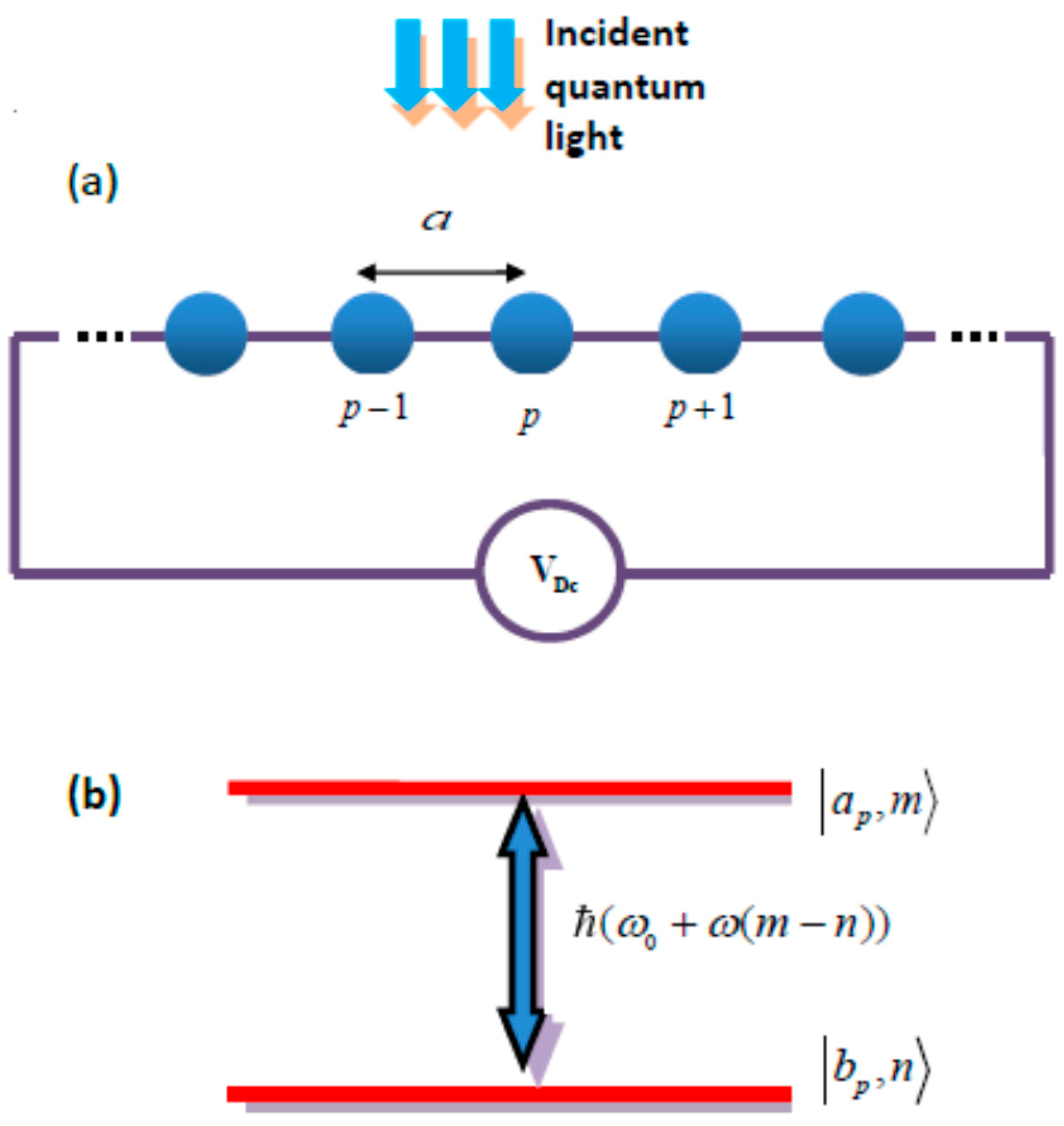
Let us consider a one-dimensional (1D) structure of identical atoms placed over a line with period a (see for example Figure 1a). Some other types of artificial atom chains are shown in Figure 2 and Figure 3. Each atom is considered as a two-level Fermion system with transition frequency . The location of the atoms in the lattice points is determined by the radius-vector , p = 0, 1, …, N, where N is a number of atoms. We assume the tunneling to be the predominant mechanism of interatomic coupling and neglect other ones (such as Förster and the radiation field transfer). As it was shown in [41], such an assumption can be justified for a wide range of realistic parameter values.
Before starting the consideration, we will discuss the potential degree of correspondence of our model to the different types of chains. Three rather conventional simplifications have been done: (i) We neglect all types of damping; (ii) we use so called rotating-wave approximation (RWA) [26]; and (iii) we assume the atomic chain to be infinitely long and perfectly periodic.
Assumption (i) relates to the case for scattering and radiation times strongly exceed the Bloch and Rabi periods. Because of RO for the quantum light are non-periodic, we imply here the value , as the Rabi-period ( is the mean number of photons). These conditions are met with a large margin in superconductor junctions (artificial fluxonium atoms) [53,54,55,56]. The damping of BO and RO in heterostructures is defined by the electron scattering and decoherence, respectively. The recent progress in molecular beam epitaxy allowed achieving the values of scattering time s in the ultra-high-quality AlGaAs/GaAs heterostructures [57]. For this case BO may be considered as ballistic, while dephasing becomes the dominant component of the damping for coherent inter-sub-band THz transitions (the typical values of characteristic times are 100–300 fs [50]). Such values are comparable with typical Bloch and Rabi periods; therefore, the damping does not manifest itself. In [50], the authors experimentally observed the manifestation of RO for the pulse with duration 200 fs, which does not exceed the dephasing time and is comparable with Rabi period (1–2 RO cycles over the pulse). For validity of our model to this case, we will consider interaction with rather short pulse, of which the duration, however, strongly exceeds the period of high-frequency filling and guaranties RWA validity.
The perfect periodicity means the identity and a rather large number of atoms in the chain. Its implementation is rather simple for 2D-heterostructures (for example, a chain of 51 element was used in experiments [50]). The problem is not so easy for QD-chains because of QDs comprise hundreds or thousands of real atoms, with inevitable variations in size and shape and, consequently, unavoidable variability in their energies and relaxation times [58,59]. One of the most promising technologies for applications in quantum photonics is the embedding of QDs within nanowires [59]. The QDs form at the apex of a GaAs/AlGaAs interface, are highly stable, and can be positioned with nanometer precision relative to the nanowire centre. As it was found [59], there is a chain of bright, nanoscale emitters in the red. QD-in-nanowire mimics very closely a two-level atom with high associated lifetime (450 ps). One more way is using a scanning tunneling microscope to create QDs with identical, deterministic sizes [58]. As it was mentioned in [58], the reached digital fidelity opens the door to QD architectures free of intrinsic broadening. This makes it reasonable to recommend our model of 1D QD-chain for visible light applications.
There exist different ways to theoretically describe complex quantum systems strongly interacted with quantum light. In quantum optics an “all-matter” picture is widely used, where the dynamics of light is integrated out (for example, in the optical Bloch equations [60,61]). In Refs. [62,63] the light-matter interaction is treated in an “all-light” picture (Lippmann-Schwinger equation approach). We use as the theoretical approach the probability amplitude method, generalized for the case of 1D chains driven via homogeneous dc field. It consists of solving of the Schrödinger equation for wave function, which is the superposition of various Wannier-Fock states for atom-light system.
To solve equations of motion for probability amplitudes analytically, we use the quasi-classical concept. The dressed electron is described as a wavepacket prepared with a well-defined quasi-momentum. The motion of quasiparticle center of mass is governed by the Newton’s law, while the internal degrees of freedom have been described by means of quantum theory, based on the concept of electron-photon entanglement widely used in quantum optics [26,27]. Thus, the position of the quasi-particle center periodically evolves with a Bloch frequency corresponding to the quasi-momentum scanning a complete Brillouin zone. Such an approach was used for BO of conductive electrons in [8,64] and will be adopted for the case of dressed electrons in this paper.
In the general case, the equations of motion were integrated numerically with simplification through RWA. However, the use of the RWA may not describe the atom-light interaction when the coupling becomes sufficiently strong (ultrastrong coupling) [65]. Both lower and upper fundamental limitations of ultrastrong coupling of atoms and light were recently formulated in [66]. We bounded our consideration by the strong coupling regime assuming the lower limitation in [66] not to be reached.
2.2. Hamiltonian in Wannier-Fock Basis
Let us denote with and , the Wannier wave functions centered at p-th atom in the excited and ground states, respectively (Figure 1). The two neighboring atoms are coupled via the electron tunneling, such that only intra-band tunnel transitions are permitted. It means that the electron due to the tunneling can go from state to state and from state to state only. The transitions between ground and excited states of different atoms are forbidden: .
Let the chain be exposed to a single-mode quantum light, which electric field operator is , where V is the normalizing volume, e is the unit polarization vector, are positive and negative frequency components of field operator, are creation-annihilation operators, respectively (an time dependence of the light is implicit). The field is assumed to be homogeneous over the chain axis. Such assumption corresponds to the chain excited by the normally incident wide laser beam, or specially-symmetric eigen-mode of microcavity, photonic crystal; etc. The chain is driven by an electrostatic (dc) field directed along the axis with responsibility for BO. We will consider the case of dipole interaction in the regime of strong coupling and assume the resonant condition to be fulfilled. The system under consideration exhibits complex single-particle BO of the electrons entangled with photons, for which the theoretical framework will be introduced.
The system is described by the total Hamiltonian (see Appendix A):
Here, the first term represents the free motion of the chain with absence of both light and dc field. It is given by , where . The second term is the Hamiltonian of free electromagnetic field. The term
is Hamiltonian of electron tunneling, are the penetration energies of potential barrier at the excited and ground states, respectively.
The component
describes the atom-light interaction, where is the interaction constant, is the dipole moment, H.c. means Hermitian conjugation. The transition dipole moments in the chain is assumed to be vectors of identical values and orientations. The operators , are creation-annihilation operators of excited state in the p-th atom. The Hamiltonian (3) is written in the RWA form [26].
The last term,
describes the driving via dc field and is responsible for BO.
2.3. Equations of Motion
The evolution of the system in the interaction picture is described by the Schrödinger equation with the interaction Hamiltonian given by:
The state vector of the “atomic chain + light” system is:
Here, , , are Fock states with n photons and Wannier states centered around p-th atom in ground and excited state, respectively, and are the unknown probability amplitudes. From the Schrodinger equation we get following equations for the probability amplitudes:
where . In the limit the System (7) and (8) goes to the corresponding equations obtained in [41] for Rabi-waves in QD chains.
2.4. Studying Observable Values
We will study the values of two types. The first ones directly characterize the spatial-temporal behavior of electronic component and therefore are averaged over photonic state distribution. They are position-dependent, thus we will address to their densities per unit cell of the chain. From among these values we introduce:
- (i)
- inversion density, given byand
- (ii)
- tunneling current density (see Appendix B)
The values of the second type directly characterize the quantum-statistical properties of light and therefore are spatially averaged. From among these values we will use:
- (iii)
- photonic number distribution
- (iv)
- mean number of photonswhere is given by (11),
- (v)
- photonic number variancewhere is given by relation (12), and
- (vi)
- von Neumann quantum entropywhere are the weights of the various Fock states of the statistical light distribution [44].
3. Approximate Analytical Solution
3.1. Preliminaries
The simplest and conventional model of BO is based on a quasi-classical approximation. It results from Equations (7) and (8) with . Electron-photon interaction disappears (subscript becomes unnecessary) and the equations become separated. The system reads,
and the same for . (the value becomes arbitrary and is taken ). In the absence of a dc field (), the eigenstate of the system corresponds to the electrons tunneling in the periodic potential and has a form of Bloch-wave , where is a phase shift per unit cell, coupled with the eigen frequency by . The phase shift is coupled with the continuous quasi-momentum via relation , conventionally restricted to the first Brillouin zone . Under the influence of a dc field, a given Bloch-state evolves up to a phase factor into the state with variation according to
or . Thus, this evolution is periodic with a Bloch frequency corresponding to the time required for the quasi-momentum to scan a full Brillouin zone. It is described by the substitution , where is the Bloch frequency, . The obtained solution relates also to the rather wide wave-packet with well-defined quasi-momentum. The periodic motion of its geometrical center corresponds to the quasi-classical model of BO.
The main idea of the analytical solution considered next is based on hypothesis that the total dynamics of quasiparticles described by Equations (8) and (9) are reducible to the superposition of two interacting partial motions: (i) internal motion, which is dictated by dressing; and (ii) external motion of the quasiparticle as a whole. The internal motion is of completely quantum origin and doesn’t allow any classical interpretation. It corresponds to the Rabi-wave and plays the role of the tunneling in the simplest case of BO considered before. The external motion is a motion of geometric center and will be described quasi-classically, following Equation (16).
3.2. Details
We consider the partial solutions of System (7) and (8) in the absence of a dc field () and the case of zero detuning (). We use the ansatz , , , , where is a given phase shift per unit cell, is the unknown eigen frequency, are unknown constant coefficients. Making use of Equations (7) and (8) we obtain for them the matrix equation
The eigenfrequencies are found from its characteristic equation
and given by
where . The correspondent eigenstates are
where
The States (14) and (15) describe the travelling of transitions between the states and along the chain (so called Rabi-waves [41]).
The periodicity of the lattice leads to a band structure of the energy spectrum of the dressed electrons in the entangled eigenstates with the corresponding eigenenergies . They are labeled by the discrete number of photons n and the continuous quasi-momentum h. Under the influence of a dc field, weak enough not to induce inter-band transitions, the state evolves up to a phase factor into the state with variation according to Equation (16). This evolution is periodic with a Bloch frequency corresponding to the time required for the quasi-momentum to scan a full Brillouin zone. It leads to the exchange,
The distribution of photonic probabilities for the state is given by
The average number of photons is
where the value is given by Relation (23). The similar elementary calculations for the state give
For photonic number variances we have
Here, von Neumann entropy [44] accumulated at the given states of light is equal for both states and given by
Due to BO, characteristics of quantum light, such as the photonic probabilities, the average number of photons, and the Neiman entropy are oscillatory functions with Bloch frequency . The amplitude of these non-monochromatic oscillations is strongly dependent on the relation between penetrations of potential barrier in the ground and excited states. In particular, as obeyed from Equation (17), for the case of identical tunneling penetrations at the ground and excited states () the value becomes constant, and oscillations vanish. The oscillating effect is suppressed likewise with the increasing of photons number n. As a consequence, a wave packet of entangled electron-photon prepared with a well-defined quasi-momentum will also oscillate in position with amplitude .
Finally, we note that there is an interesting ability for quantum state control via adiabatically turning the dc field on and off. Starting from we proceed to turn on until its maximal value. Thereafter we slowly turn off and end it at the moment . This process corresponds to the turning the phase from initial value until the final one given by
The optimal choice of the turning time T makes the arbitrary value of the phase turn reachable. As a result, the DC field via BO becomes an effective tool of control of quantum light statistics. In particular, the photonic probabilities, degree of electron-photon entanglement, and Neumann entropy may be adiabatically changed from minimal to maximal values (and vice versa) via adiabatic turning of the DC field.
4. Numerical Modelling and Discussion
In this section, we will show and discuss the numerical results for the different types of initial states. The System (8) and (9) was solved with the Crank-Nicolson numerical integration technique [67]. We have used periodic Born-Von Karman relations as boundary conditions [41]. Let us note that the concrete form of boundary conditions has no physical importance in our case because the area of oscillations is placed rather distantly from the ends of the chain. For simplicity, we will limit our consideration by the case of zero detuning ().
We will consider three types of initial conditions. For two of them the electron and photon subsystems are assumed to be initially non-interacting. The electronic subsystem is prepared as a coherent superposition of Gaussian wave packets:
where are arbitrary complex values that satisfy the normalization condition, are the position of Gaussian center, effective Gaussian width, and the initial value of quasi-momentum at the ground and excited states, respectively.
The photonic subsystem is prepared in the next types of state:
(i) Coherent initial state; It is given by Poisson distribution , where is the mean number of photons. The total wavefunction at the moment t = 0 is given by
(ii) Vacuum initial state; It is given by the total wave function
where are the arbitrary coefficients satisfying normalization condition;
(iii) Entangled photon-electron initial state; The electron-photon entanglement prepared initially before the driving fields would be switching on. The initial condition reads
where is normalization constant. The value of inversion for the State (34) is equal to zero.
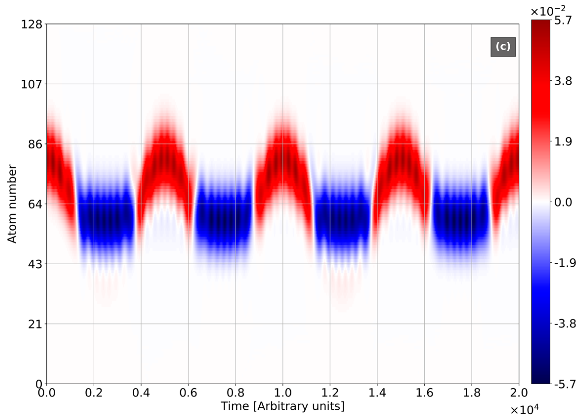
In Figure 4, we plotted the temporal dynamics of inversion. The case of zero dc field and coherent initial light (Figure 4a) corresponds to the well-known scenario of collapse-revivals given by the Jaynes-Cummings model for the single atom [26]. The initial spatial distribution is not disturbed over the motion via inter-atomic tunneling. For the case of dc field existence and coherent initial light (Figure 4b), the collapse-revivals picture drifts due to BO: The collapses and revivals appear at the different segments of the atomic chain. The inversion behavior dramatically changes for the vacuum state of light (Figure 4c). Here, BO leads to the separation of areas of positive and negative values of inversion. The particle in the excited state (positive inversion) exhibits the single oscillation of rather high amplitude in the course a half of Bloch circle. During the other part of Bloch circle, the particle is in rest, which means its appearance in the ground state (negative inversion). The reason for this is the weak value of transparence of potential barrier at the ground level used in the shown calculations. In contrast with single atom scenario, vacuum RO between maximal and minimal values of inversion occurs with Bloch frequency instead of Rabi frequency .
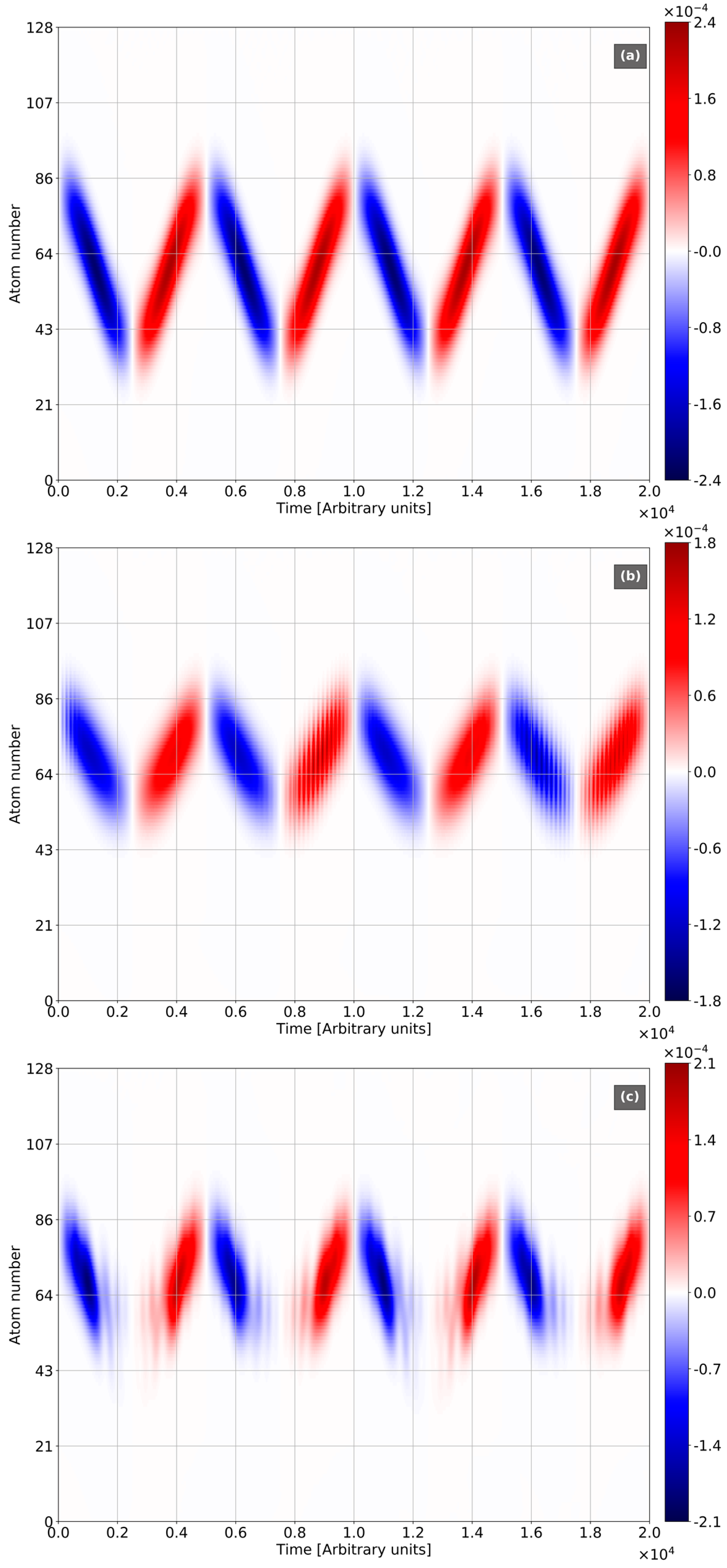
In Figure 5, we plotted the time dependence of the tunneling current. For the absence of light (Figure 5a), the current exhibits the periodic dynamics with Bloch frequency. This picture is dramatically changed due to the light-chain coupling both for coherent and vacuum states of light (Figure 5b,c), respectively. For the coherent light, the tunnel current is modulated in exact compliance with the collapse-revivals picture. This result is rather counterintuitive; it demonstrates the influence of the quantum-light statistics on the low-frequency motion of the charges driven separately by a dc field. It makes the spectra of the tunneling current more wide and various wherewith in the case of ordinary BO. It opens a new promising avenue in the spectroscopy of nano-circuits and nano-devices based on the synthesis of quantum optical and dc tools of control [51,52]. For the vacuum state of light, the tunnel current periodically evolves through one pulse after another with frequency instead of continuous periodic behavior in the case of ordinary BO [8,9,10,11,12,13,14,15,16,17,18,19,20,21,22,23,24,25]. Such evolution is accompanied by the modulation with Rabi frequency. The results demonstrate high and various mutual interactions of RO and BO.
In Figure 6, we plot the dynamics of mean number of photons. Again, we see the mutual influence of RO and BO. For dc field absence (Figure 6b), the collapse-revivals scenario corresponds the Jaynes-Cummings model for single atom [26]. It represents the quantum interference of the spectral components with different Rabi-frequencies and different relative amplitudes [26]. For dc field appearance (Figure 6a), there is one more type of interference components with frequencies ( is integer value). Among them, the term with is dominant, and its amplitude is comparable with RO components. As a result, the mean number of photons is modulated with Bloch frequency . Therefore, the dc field via BO opens one more way of engineering of the quantum light states. This effect depends on the large number of physical factors, such as dc field value, energy and dipole moment of quantum transition for the atom, tunnel coupling, etc. Concluding, the results of numerical modeling agree with the simple analytical model, developed in Section 3. They are promising for different applications in quantum computing, quantum informatics, etc.
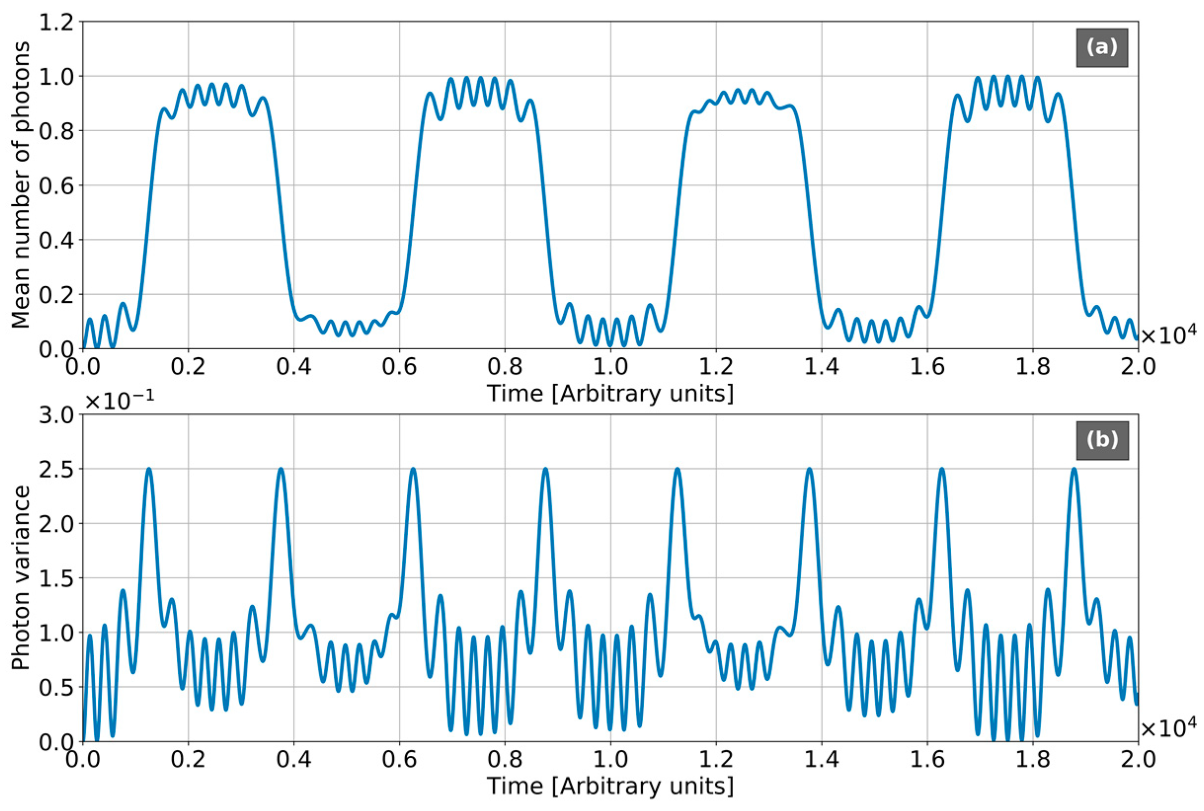
Figure 7 shows the quantum-statistical properties of light. The temporal behavior of the mean number of photons (Figure 7a) may be rather simply understood from the quasi-classical point of view developed in Section 3. The processes of photons emission and absorption correspond to the rapid jumps from value to (and vice versa). Comparing Figure 7a with Figure 4c, one can see these jumps occurrence in a small vicinity of the stops and turns of the wavepacket. The neighboring stopping points are separated in time by half of a Bloch circle. Sufficiently far from a stopping point, the motion is characterized by rather small acceleration. It means the existence of rather weak fluctuations of photonic number, dictated by RO and taking place with Rabi-frequency . This scenario dramatically differs from RO in the single atom, where the acts of photons emission-absorption correspond the harmonic oscillations with Rabi-frequency.
Figure 7b displays the evolution of photonic variance. As it was mentioned above, the electrons and photons in the initial state are uncorrelated. Thus, electron-photon entanglement is poor at the intervals of motion between the stopping points, whereby the variance oscillates only due to photon number fluctuations of rather small amplitude with vacuum Rabi-frequency. The processes of photons emission-absorption are accompanied the strong narrow peaks of variance. Thus, the vicinities of stopping points are characterized by the strong non-classicality of light and high degree of its entanglement with electronic sub-system. This scenario strongly differs from the case of the harmonic oscillations of variance with Rabi-frequency for the single atom [26]. The obtained results show that such manifestations of non-classicality of light, such as electron-photon entanglement and accumulated entropy become controllable by dc field via BO. As it is well known [26], the physical origin of vacuum RO is a manifestation of spontaneous emission of the single exited state in strong coupling regime. The obtained dynamics qualitatively support the conclusion of an early paper [68], that BO dramatically changes the physical picture of spontaneous emission in the atomic chains.
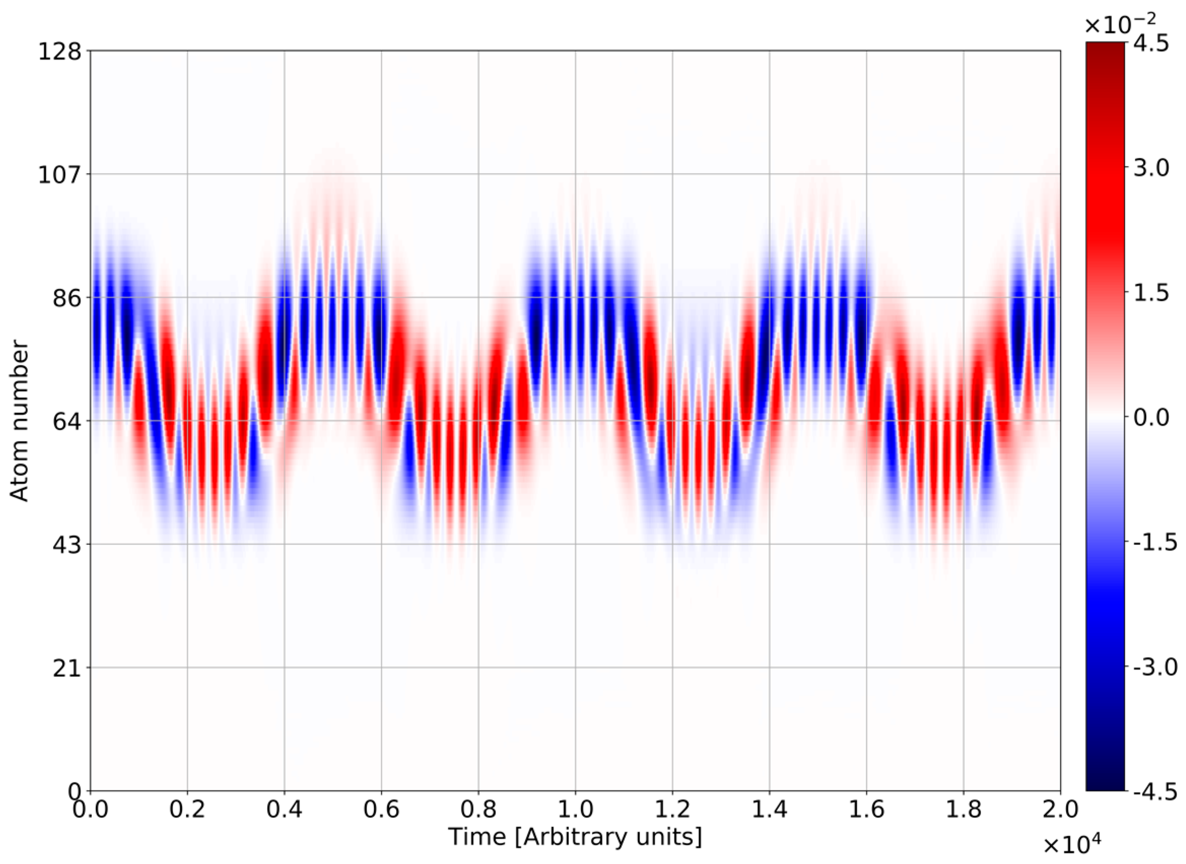
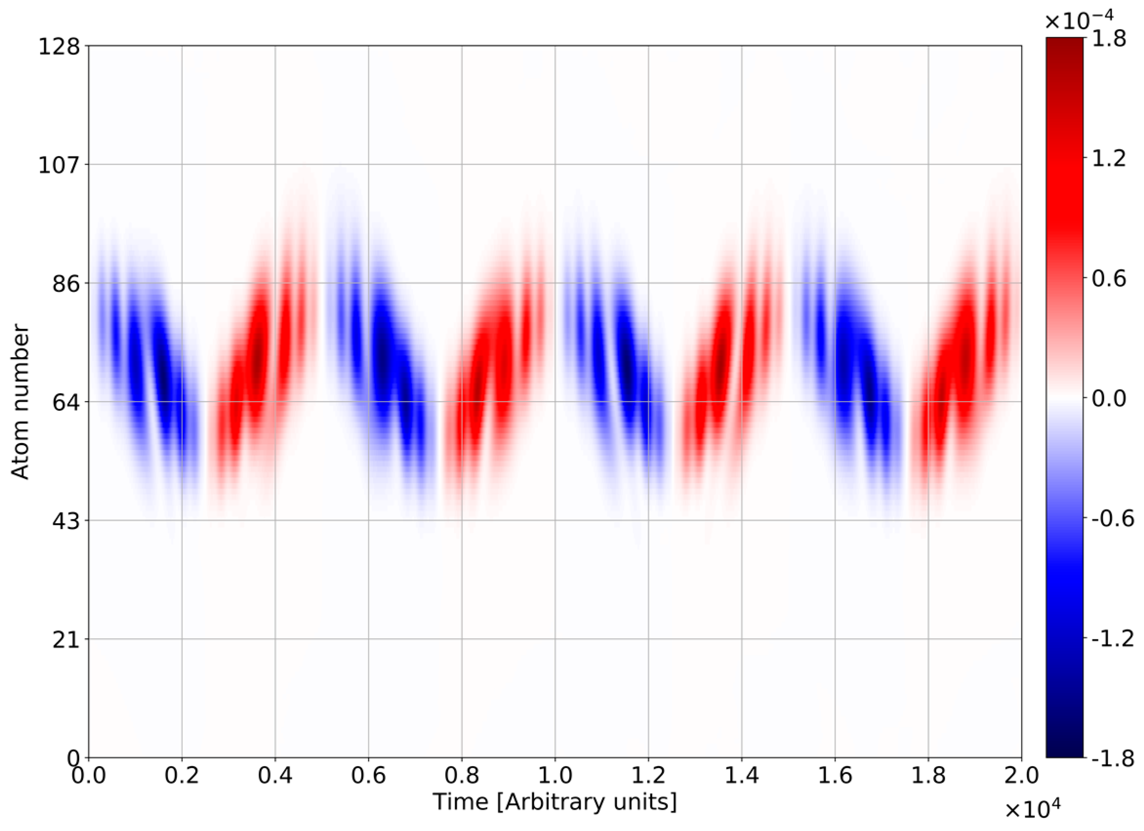
To illustrate the mutual influence of high-frequency and low-frequency motions, we show the spatial-temporal evolution of inversion for initial condition (34) (Figure 8). One finds out of the phase oscillations of inversion with Bloch frequency. The two halves of every Bloch period correspond to the excited and ground state, respectively. Here, BO of inversion is modulated with RO. Such dynamics are similar to the shown for the vacuum initial state at Figure 4c, however, the modulation depth strongly increases due to the influence of initial entanglement (the inversion evolves over the single Rabi-circle between zero and ). In Figure 9, we show the tunnel current for initial state (34), which as well as inversion exhibits the high level of RO modulation. Comparing it with Figure 5c, one finds again the strong influence of initial electron-photon correlations.
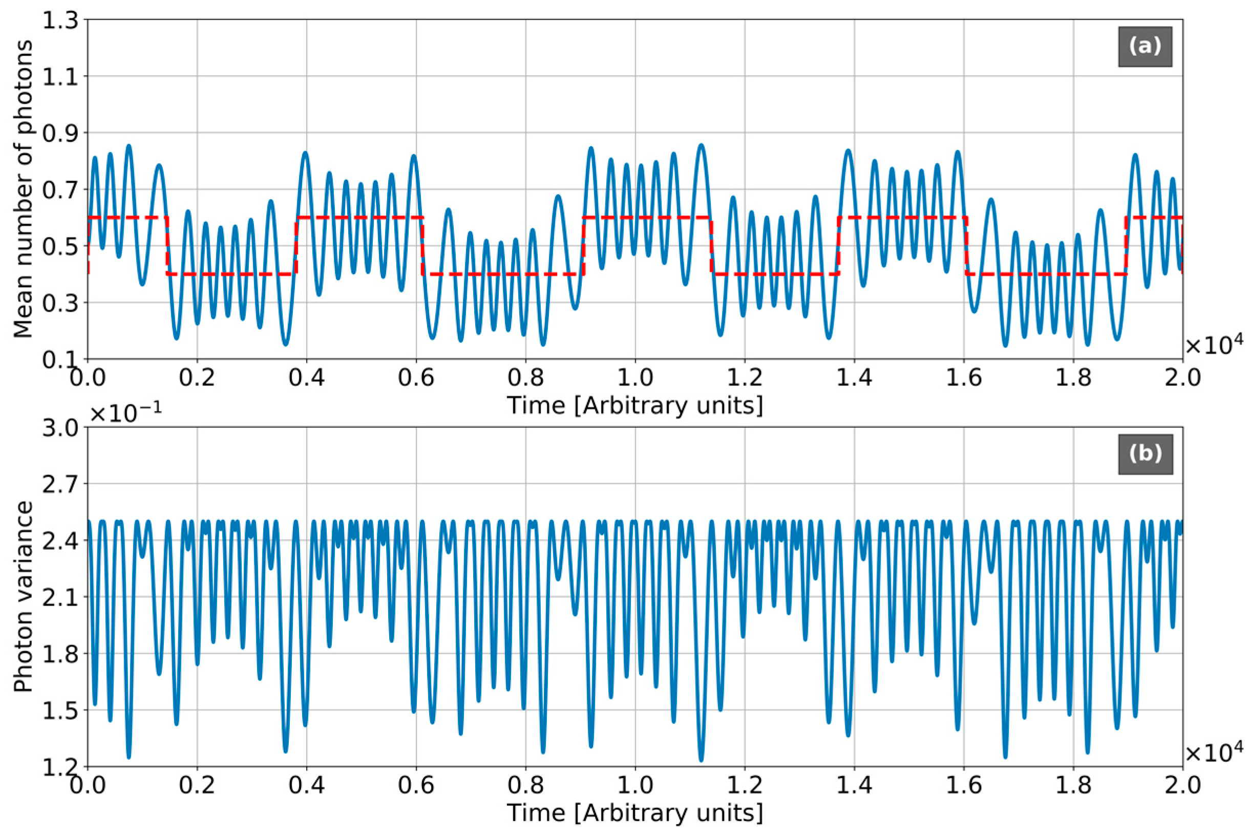
Figure 10 displays the quantum-statistical properties of light. The evolution of mean number of photons (Figure 10a) may be considered as a periodic system of step-like beatings (dashed line), modulated with high-frequency oscillations (solid curve). The value averaged with respect to the step-period is approximately equal to 0.5, which is equal to the main photon number for both states given by Equations (20) and (21). The general physical interpretation of Figure 10a may be done from the quasi-classical point of view as an interference of this states (of course, we speak here about moving wavepackets, but not about perfect travelling waves). Again, the photon emission-absorption with Bloch-period takes place in the vicinity of stopping points. One can see, comparing Figure 10a with Figure 9, that the moments of shut-down are agreed with zeros of inversion. Translatory motion of the wavepacket is accompanied by RO between eigenstates, which correspond to high-frequency fluctuations with Rabi-frequency. In Figure 10b we plot the dynamics of photonic variance. In contrast with vacuum photonic state, the variance is maximal at the intervals of translatory motion and strongly decreases in the vicinities of stopping points. The reason for it is that translatory motion corresponds to the statement in one of the Eigenstates (20) and (21). Every one of these states is characterized by the maximal level of electron-photon entanglement. Photons emission-absorption means the mutual transformation of the States (20) and (21). It leads to creation the coherent superposition of these states for a short time with comparable probability amplitudes. It leads to the breaking of electron-photon correlations. Again, RO-fluctuations are imposed to this ideal picture similar to the case of the vacuum photonic state. The photonic variance in these oscillations reaches the value , which corresponds to the maximal one for two States (20) and (21).
5. Some Other Potential Experimental Implementations
5.1. Semiconductor 2D-Heterostructures
The next promising candidate for the experimental implementation of the model considered above is the low-dimensional semiconducting heterostructure (see Figure 2) under femtosecond inter-sub-band excitation [50]. For example, the sample consisting of 51 GaAs quantum wells separated by barriers was implemented in [50]. A coherent excitation of the sample was created by a femtosecond pulse with a center frequency resonant to the inter-sub-band transition. The resonant line at 30 THz was homogeneously broadened with coherence time 320 Fs. The amplitude of incident field was varied inside of area (5–50) kV/cm. As a result, there were observed coherent sub-picosecond RO and manipulated in a wide range by varying the strength of the coherent driving field. The measurements [50] qualitatively agreed with the predictions of the simplest model based on Maxwell-Bloch equations for non-interactive two-level systems. Conventional simplifications, such as RWA and omitting of all types of damping have been used. The simulation of the pulse driving field was done by varying the Rabi frequency .
Here, we add the dc field for manipulation by atomic chain via BO. For the application of our model to the potential experiments with 2D-heterostructures, it is necessary to describe the driving quantum light as a short transient normally incident to the heterostructure. The driving process in this case is described by the instantaneous coupling coefficient g. The field quantization should be modified following Appendix C. The quantum properties of light in the wavepacket are dictated by the special pair of bosonic creation-annihilation operators, which allows us to rewrite the dynamic Equations (7) and (8) as:
where , is a slow envelope of the driving pulse.
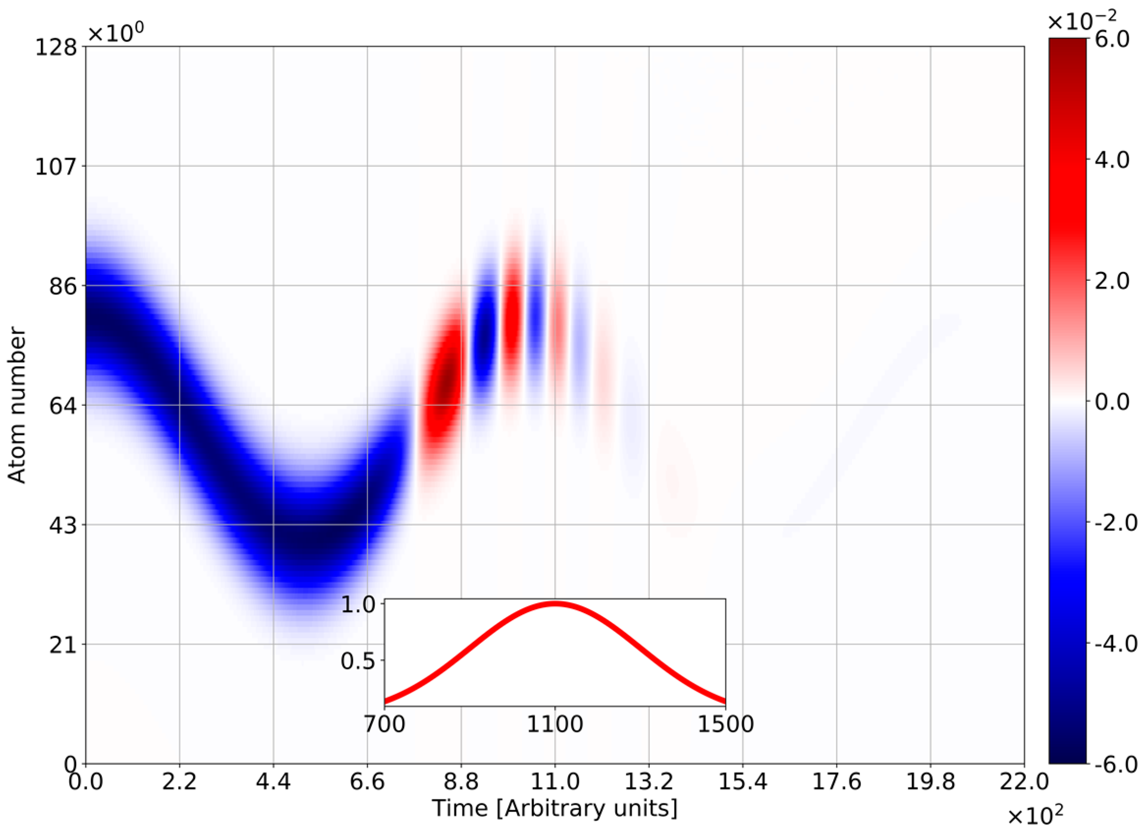
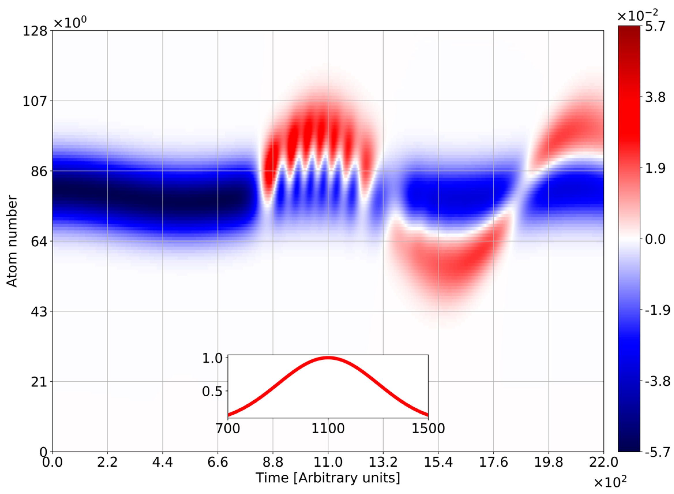
The driving with electromagnetic pulse leads to chain dynamics qualitatively different from the case of monochromatic light. Figure 11 and Figure 12 depict the temporal-spatial evolution of inversion for different relations between barrier penetrations at 1S and 2S levels. Figure 11 shows the case of identical penetrations. One finds BO over the pulse duration. The oscillations are modulated with Rabi frequency and stop with the pulse disappearing at zero inversion. The behavior becomes quite different for the case of 2S penetration strongly exceed 1S one. (Figure 12). No oscillations exist before the pulse appearance (). The reason for this is a weak value of penetration at 1S level. The switching of pulse creates both RO and BO. The RO existence is limited by the pulse duration (), while BO continues even after the pulse switches off. It is a result of tunneling at the 2S-level on which the penetration is much higher. The charge existence at the 2S-level is a result of resonant pumping by the optical pulse. Thus, we can consider the resonant pumping as a tool of BO triggering and speak about photon-assisted BO.
5.2. Josephson Junction
The next promising candidate for experiment implementation is a single Josephson junction embedded in an inductive environment. As it was shown in [53,54,55,56], the voltage-biased Josephson junction exhibits the temporal dynamics equal to the motion of a fictitious charged particle with inertia provided by the inductance. This particle moves in a potential, which also has a periodic part and a linear tilt. On the other hand, a Josephson junction strongly coupled to the microwave resonator (Figure 3) in the resonant regime may be considered as an artificial two-level atom (“fluxonium” [54]). It is described by the Jaynes-Cummings model [54] and exhibits RO dynamics [54]. Here, we will focus on the case of Josephson junction simultaneously driven by dc voltage and quantum light in the regime of small detuning. We will show that the model investigated in this work is applicable to this type of physical system. Therefore, we will start our analysis by identifying the parameters of Josephson junction in terms of this model.
The temporal dynamics of entire circuit may be described using so-called quasi-charge representation [53,55]. Let us first consider the single junction, of which the standard form reads , where , are operators of junction charge and phase difference across the junction, respectively. It describes the particle of mass moving in the periodic potential [55] ( is a junction capacitance). The eigenfunctions of this Hamiltonian are Floquet-Bloch modes with condition of quasi-periodicity , where is periodic function, is a number of the gap. These functions describe the motion of the quasiparticles, which is similar to the motion of electrons in crystal. The phase and quasi-charge Q play the role of the conjugated spatial coordinate and quasi-momentum for electrons in crystals, respectively. The energies of the two first modes , are separated by the gap, which in the regime of interest here (, ) is of the order of plasma frequency . Taking GHz, and , we have GHz. Next, in the limit the energy bands are purely sinusoidal [53] with the bandwidths of the order of [55]
(the typical values are GHz). The situation is the same in the case of atomic chain considered above (see Equation (13) in the case ). Thus, we are able to establish the correspondence .
The additional series inductance and switching on the bias voltage transforms the Hamiltonian to
where is the constant of inductance energy, is the total phase difference across the circuit, which is determined by the bias voltage , such that [53].
The case under consideration has a simple physical interpretation based on the charge-phase duality [53]. The voltage-biased junction with inductive environment and the current-biased junction shunted by a capacitor are dual to each other when exchanging the role of quasi-charge and phase. The dynamics of the circuit, shown in Figure 3, are equal to the intra-band motion of a fictitious charged particle in the tilted periodic potential. The tilt leads to BO of the particle in the quasi-charge space, which allows for the identification of the Bloch-frequency as dual plasma frequency .
The inductive strong coupling of a Josephson junction with a microwave resonator leads to its dressing with microwave photons. It corresponds to the periodic emission-absorption of photons and inter-band transitions by the fictitious charged particle (RO). Thus, the qualitative picture of junction behavior is similar to the BO of dressed electrons considered above: The periodic inter-band transitions (RO of fluxonium) are accompanied by the charge oscillations through the bias-voltage driving. For formal identification of the coupling parameters of the system, “junction + microwave resonator”, it is necessary to analyze in more detail the total Hamiltonian. It reads
where is a Hamiltonian of the Josephson junction in an inductive environment, is Hamiltonian of microwave photons in the resonator, is a Hamiltonian of junction-cavity interaction, and is a support of biased voltage. For further analysis, it is convenient to use the secondary quantization technique. The Hamiltonian of photons reads
where , , are creation-annihilation operators for microwave photons, which satisfy the conventional bosonic commutative relations. By following the concept of quasi-charge-phase duality, the Fourier-Bloch states exchanged by the Wannier functions (see Appendix A) and the Hamiltonian is written in the Wannier-basis. We denote the two first states with quasi-charge Q as and and introduce the raising operators and . The atomic Hamiltonian may be rewritten as , where is Pauli inversion matrix.
For junction-cavity interaction we have [54]
where , is the matrix element of effective dipole moment. The Hamiltonian is written in rotating-wave approximation. It is equal to the Hamiltonian (3) if the coupling coefficient identified with the value
where is the quantum of resistance. The validity of rotating-wave approximation implies all relevant energies to be smaller than the plasmonic frequency of the Josephson junction and resonant frequency of resonator. In particular, we impose the characteristic energy, , associated with the inductance to be smaller than . It corresponds to the values nH, which are quite reachable [56]. Second, we need also . For standard value [56] we have for this condition been imposed. The coherence time and energy relaxation time both are of the order [56]. Thus, the number of BO flops is high enough for their experimental observation in the fluxonium atom in microwave frequency range. The real cases may be described by lossless model considered above.
6. Conclusion and Outlook
In this paper, we developed a model of the chain of two-level artificial atoms manipulated simultaneously by a dc field and single-mode quantum light in the strong coupling regime. Atom-light interactions were assumed to be resonant. The cases of monochromatic light and light pulse have been considered. Both, electronic and photonic characteristics of the oscillation process, have been studied, such as: (i) inversion density; (ii) tunneling current density; (iii) distribution of photon probabilities; (iv) mean number of photons; (v) photon number variance; and (vi) Neumann entropy of light. The different types of the initial states of the light have been considered: (i) coherent state; (ii) vacuum photonic state; and (iii) Fock-state entangled with the electron wave packet. The Gaussian wavepackets were chosen as initial states of atoms.
The model is universal with respect to the physical origin of artificial atoms and frequency ranges of atom-light interaction. The model was adapted to the semiconductor 2D-heterostructures (THz frequencies), semiconductor quantum dots (optical range), and Josephson junctions (microwaves). The initial data for numerical simulations are taken from recently published experiments.
The dynamical equations have been studied both analytically and numerically. The idea for analytical simplification is based on the separate description of electrons dressing with photons and quasi-classical motion of their geometrical center driven by a dc field. The analytical solutions are in good qualitative agreement with numerical simulations. Our model is based on such conventional simplifications as neglect of damping and RWA. Their validity for considered systems was supported by numerical estimations taken from experimental data.
The following conclusions are emerged from our studies:
- (1)
- The case of initial coherent state of the light exhibits the collapse-revival picture, which drifts over the chain (collapses and revivals placed in the different spatial areas). In contrast with Jaynes-Cummings model, the collapse-revival picture is modulated with Bloch frequency;
- (2)
- In the case of initial vacuum state of light, the photon emission and absorption occurs with Bloch frequency, instead of Rabi-frequency in Jaynes-Cummings model. The photonic probabilities are mainly modulated with Bloch frequency, while the contribution of Rabi-components is rather slight. BO strongly squeezes the vacuum state of light entangled with electronic wavepackets;
- (3)
- The electron-photon entanglement dramatically modifies the tunnel current behavior. It becomes modulated agreed with the collapse-revival picture for the case of coherent state of light, and periodically modulated by RO for the case of initial photonic vacuum;
To conclude, the main result of the paper is the novel effect of the influence of BO and quantum statistical properties of light on each other. It is counterintuitive because of the strongly different frequency ranges for such types of oscillations existence. The reason for it is an entanglement of electronic and photonic states in the system been considered.
The obtained results allow for the control of quantum-statistical properties of light via adiabatically turning the dc field. They are promising for applications in quantum optics, quantum informatics, and quantum computing. The mutual modulation of low-frequency BO and high-frequency inter-band transitions produces the new types of spectral lines in tunneling current and optical polarization. It opens the promising ways in spectroscopy of nanodevices in THz and optical frequency ranges. These problems may be considered as directions for future research activity.
Author Contributions
Developments of the physical models, derivation of the basis equations, interpretation of the physical results and righting the paper have been done by I.L. and G.S. jointly. The Numerical Python calculations and Matplotlib figures were produced by I.L.
Acknowledgments
G.S. acknowledges support from the project FP7-PEOPLE-2013-IRSES-612285 CANTOR. We gratefully acknowledge the stimulating discussions with Professor Dmitry Mogilevtsev.
Conflicts of Interest
The authors declare no conflicts of interest.
Appendix A. Derivation of Hamiltonian in the Wannier-Fock Basis
The Hamiltonian of conductive electron movement in the chain associated with the interatomic tunneling, which is described by the periodic potential , is
The eigenmodes of Hamiltonian (A1) are two Bloch modes correspondent to valence (b) and conductive (a) zones and denoted as , = a, b, h being a scalar quasi-momentum directed along the chain. Because the electrons are strongly confined inside the atoms, we will use as a basis, Wannier functions [69], defined as a linear combinations of Bloch modes
Let us mention some properties of Wannier functions, which are important for our analysis. Wannier function is strongly localized inside the j-th atom. Inversion of Equation (A2) gives the expression of Bloch states in the terms of Wannier functions:
Wannier functions satisfy the orthogonality relation .
Projecting on the Bloch modes and using (A3), we obtain the dispersion law for free-tunneling electron in the next form:
Denoting
we can rewrite (A4) in the following form:
The Hamiltonian (A1) may be presented with the Wannier basis in the form of a block diagonal matrix
with diagonal-on elements
where . The tunneling coupling exist only between the neighboring atoms (tight-binding approximation). Thus, we omit for brevity the spatial arguments in tunneling matrix elements: , . The Hamiltonian (A7) subject to (A8) reads
Hamiltonian (A9) in the secondary quantization form is equivalent to the sum of intra-level term and tunneling Hamiltonian.
The total Hamiltonian may be presented as , where the second component corresponds to the free single-mode photons motion, and are creation and annihilation operators of photons. We describe the atom-photon interaction in the dipole approximation by the third term [26], where
is the single-mode quantum light operator of electric field, V is the normalizing volume, and e is the unit polarization vector.
The quantum state of light will be described in terms of photons number states (Fock-states) . The basis states should be used in our analysis correspond to the independent photons number states and Wannier electrons (Wannier-Fock basis). Let us proceed to the calculation of matrix elements
Let us shift the origin for a given j to the center of the j-th atom via the relation . Using the Wannier functions orthogonality for different electron bands, we have . Together with orthogonality of the Fock states it makes (A11)
Here is the matrix of the dipole moments, . The second term at the top line characterizes quantum transitions in the separate atom. For real atoms (excluding hydrogen) only off-diagonal elements, are non-zero due to the inversion symmetry [70]. For some types of artificial atoms (such as quantum dots) the inversion symmetry is not obligatory. In this case on-diagonal elements of dipole matrix may be non-zero [37], which corresponds to the special type of intra-level motion [37]. The middle line in (A12) corresponds to the interaction of neighboring atoms stimulated by photons (photon-assistant tunneling over the same level).
The last term describes the dipole interaction of the chain with the dc field. Its matrix elements are
Using the orthogonality of Wannier states, we obtain
The first term in the top line corresponds to BO, the second one describes the Stark-effect [70].
Appendix B. Derivation of Formula for Tunneling Current
For calculating the tunneling current we introduce the operator of the particle number in the j-th atom and formulate the equation of continuity
where is the current density operator in the j-th atom and the left-hand part in (A15) is a discrete analog of divergence in 1D-case. These operators act only to the electronic states; therefore all relations of this Appendix are given in terms of Wannier states. Using Heisenberg equation for the operator , we rewrite (A15) in the form
The tunneling currents over excited and background energy levels are independent, thus . Using (A16) we obtain
where
is a component of the Hamiltonian (2), chargeable for the tunneling at the excited level (the similar equation may be written for the Hamiltonian ). Using (A18), we calculate the commutator in the right-hand part of (A17) and obtain
It corresponds to the operator of the tunneling current at the excited level
The observable value of the tunneling current is
Using the approximation , and adding the similar support of the ground level, we obtain Relation (10). This relation corresponds to the well-known definition of the probability flow in 3D continuous case [70].
Appendix C. Quantization of Electromagnetic Fields in Wavepackets
For the secondary quantization in the wavepacket we use the method proposed by Keller [71]. First, we consider the linearly polarized electric field to have the spatial-temporal dependence for a 1D cavity resonator [26]. We assume the cavity formed by two parallel perfectly conductive planes distanced on the length L. The positive-frequency part of electric field operator is given [26]
where V is normalization volume, , is an integer value, .
Next, following [71], we introduce the special complete system of basis classical wavepackets , every one of which is given by the superposition of cavity modes
where are elements of unit matrix with conventional unitary condition , is the Kronecker delta. Equation (A22) using (A23) may be rewritten as
Using (A24) and unitary condition, we obtain
where is a new set of creation-annihilation operators, satisfying the Bose commutative relations . The basis wavepackets are non-orthogonal:
The field Hamiltonian is
Due to the property (A26), the energies of different modes are mixed via their mutual interference.
For applying the single mode approximation, some additional simplifications should be done. Let us assume that we consider the non-monochromatic field with the narrow frequency spectrum, which were localized in the vicinity of central frequency . In this case the different modes become approximately orthogonal and their interference disappears. The model of the wavepacket in the first order of dispersion theory gives
where is a slow envelope, the exponential factor gives the high-frequency filling, and is a group velocity. The approximate field Hamiltonian and electric field operator read
respectively, where are annihilation-creation operators for photon in the wavepacket. The coupling factor becomes time-dependent, which allows us to consider the case of driving light in the form of the rather long laser pulse (assumed that the pulse duration strongly exceeds the period of high-frequency filling, which guarantees the RWA validity in our model).
References
- Bloch, F. UЁ ber die Quantenmechanik der Elektronen in Kristallgittern. Z. Phys. 1929, 52, 555–600. [Google Scholar] [CrossRef]
- Zener, C. A theory of electrical breakdown of solid dielectrics. Proc. R. Soc. Lond. 1934, 145, 523–529. [Google Scholar] [CrossRef]
- Wannier, G.H. Wave functions and effective Hamiltonian for Bloch electrons in an electric field. Phys. Rev. 1960, 117, 432. [Google Scholar] [CrossRef]
- Wannier, G.H. Stark ladder in solids? A reply. Phys. Rev. 1969, 181, 1364. [Google Scholar] [CrossRef]
- Kuehn, W.; Gaal, P.; Reimann, K.; Woerner, M.; Elsaesser, T.; Hey, R. Coherent Ballistic Motion of Electrons in a Periodic Potential. Phys. Rev. Lett. 2010, 104, 146602. [Google Scholar] [CrossRef] [PubMed]
- Waschke, C.; Roskos, H.; Schwedler, R.; Leo, K.; Kurz, H.; Köhler, K. Coherent submillimeter-wave emission from Bloch oscillations in a semiconductor superlattice. Phys. Rev. Lett. 1993, 70, 3319. [Google Scholar] [CrossRef] [PubMed]
- Preiss, P.M.; Ma, R.; Tai, M.E.; Lukin, A.; Rispoli, M.; Zupanic, P.; Lahini, Y.; Islam, R.; Greiner, M. Strongly correlated quantum walks in optical lattices. Science 2015, 347, 1229–1233. [Google Scholar] [CrossRef] [PubMed] [Green Version]
- Gluck, M.; Kolovsky, A.R.; Korsch, H.J. Wannier–Stark resonances in optical and semiconductor superlattices. Phys. Rep. 2002, 366, 103–182. [Google Scholar] [CrossRef] [Green Version]
- Ben Dahan, M.; Peik, E.; Reichel, J.; Castin, Y.; Salomon, C. Bloch Oscillations of Atoms in an Optical Potential. Phys. Rev. Lett. 1996, 76, 4508. [Google Scholar] [CrossRef] [PubMed]
- Madison, K.W.; Fischer, M.C.; Diener, R.B.; Niu, Q.; Raizen, M.G. Dynamical Bloch Band Suppression in an Optical Lattice. Phys. Rev. Lett. 1998, 81, 5093. [Google Scholar] [CrossRef]
- Morsch, O.; Muller, J.H.; Cristiani, M.; Ciampini, D.; Arimondo, E. Bloch Oscillations and Mean-Field Effects of Bose-Einstein Condensates in 1D Optical Lattices. Phys. Rev. Lett. 2011, 87, 140402. [Google Scholar] [CrossRef] [PubMed]
- Bongs, K.; Sengstock, K. Physics with Coherent Matter Waves. Rep. Prog. Phys. 2004, 67, 907. [Google Scholar] [CrossRef]
- Ferrari, G.; Poli, N.; Sorrentino, F.; Tino, G.M. Long-Lived Bloch Oscillations with Bosonic Sr Atoms and Application to Gravity Measurement at the Micrometer Scale. Phys. Rev. Lett. 2006, 97, 060402. [Google Scholar] [CrossRef] [PubMed]
- Battesti, R.; Cladé, P.; Guellati-Khélifa, S.; Schwob, C.; Grémaud, B.; Nez, F.; Julien, L.; Biraben, F. Bloch Oscillations of Ultracold Atoms: A Tool for a Metrological Determination of h/mRb. Phys. Rev. Lett. 2004, 92, 253001. [Google Scholar] [CrossRef] [PubMed]
- Morandotti, R.; Peschel, U.; Aitchison, J.S.; Eisenberg, H.S.; Silberberg, Y. Experimental Observation of Linear and Nonlinear Optical Bloch Oscillations. Phys. Rev. Lett. 1999, 83, 4576. [Google Scholar] [CrossRef]
- Pertsch, T.; Dannberg, P.; Elflein, W.; Bräuer, A.; Lederer, F. Optical Bloch Oscillations in Temperature Tuned Waveguide Arrays. Phys. Rev. Lett. 1999, 83, 4752. [Google Scholar] [CrossRef]
- Peschel, U.; Pertsch, T.; Lederer, F. Optical Bloch oscillations in waveguide arrays. Opt. Lett. 1998, 23, 1701–1703. [Google Scholar] [CrossRef] [PubMed]
- Zheng, M.J.; Xiao, J.J.; Yu, K.W. Controllable optical Bloch oscillation in planar graded optical waveguide arrays. Phys. Rev. A 2010, 81, 033829. [Google Scholar] [CrossRef]
- Bromberg, Y.; Lahini, Y.; Silberberg, Y. Bloch Oscillations of Path-Entangle Photons. Phys. Rev. Lett. 2010, 105, 263604. [Google Scholar] [CrossRef] [PubMed]
- Afek, I.; Natan, A.; Ambar, O.; Silberberg, Y. Quantum state measurements using multipixel photon detectors. Phys. Rev. A 2009, 79, 043830. [Google Scholar] [CrossRef]
- Afek, I.; Ambar, O.; Silberberg, Y. High-NOON States by Mixing Quantum and Classical Light. Science 2010, 328, 879–881. [Google Scholar] [CrossRef] [PubMed]
- Sanchis-Alepuz, H.; Kosevich, Y.A.; Sanchez-Dehesa, J. Acoustic Analogue of Electronic Bloch Oscillations and Resonant Zener Tunneling in Ultrasonic Superlattices. Phys. Rev. Lett. 2007, 98, 134301. [Google Scholar] [CrossRef] [PubMed]
- Anderson, B.P.; Kasevich, M.A. Macroscopic quantum interference from atomic tunnel arrays. Science 1998, 282, 1686–1689. [Google Scholar] [CrossRef] [PubMed]
- Kudo, K.; Monteiro, T.S. Theoretical analysis of super–Bloch oscillations. Phys. Rev. A 2011, 83, 053627. [Google Scholar] [CrossRef]
- Hartmann, T.; Keck, F.; Korsch, H.J.; Mossmann, S. Dynamics of Bloch oscillations. New J. Phys. 2004, 6, 2. [Google Scholar] [CrossRef]
- Scully, M.O.; Zubairy, M.S. Quantum Optics; Cambridge University Press: Cambridge, UK, 2001. [Google Scholar]
- Cohen-Tannoudji, C.; Dupont-Roc, J.; Grynberg, G. Atom-Photon Interactions: Basis Properties and Applications; Wiley: Chichester, UK, 1998. [Google Scholar]
- Rabi, I.I. Space Quantization in a Gyrating Magnetic Field. Phys. Rev. 1937, 51, 652. [Google Scholar] [CrossRef]
- Hocker, G.B.; Tang, C.L. Observation of the Optical Transient Nutation Effect. Phys. Rev. Lett. 1968, 21, 591. [Google Scholar] [CrossRef]
- Johnson, T.A.; Urban, E.; Henage, T.; Isenhower, L.; Yavuz, D.D.; Walker, T.G.; Saffman, M. Rabi flopping between ground and Rydberg states with dipole-dipole atomic interactions. Phys. Rev. Lett. 2008, 100, 113003. [Google Scholar] [CrossRef] [PubMed]
- Kamada, H.; Gotoh, H.; Temmyo, J.; Takagahara, T.; Ando, H. Exciton Rabi Oscillation in a Single Quantum Dot. Phys. Rev. Lett. 2001, 87, 246401. [Google Scholar] [CrossRef] [PubMed]
- Blais, A.; Huang, R.-S.; Wallraff, A.; Girvin, S.M.; Schoelkopf, R.J. Cavity quantum electrodynamics for superconducting electrical circuits: An architecture for quantum computation. Phys. Rev. A 2004, 69, 062320. [Google Scholar] [CrossRef] [Green Version]
- Gambetta, J.; Blais, A.; Schuster, D.I.; Wallraff, A.; Frunzio, L.; Majer, J.; Devoret, M.H.; Girvin, S.M.; Schoelkopf, R.J. Qubit-photon interactions in a cavity: Measurement-induced dephasing and number splitting. Phys. Rev. A 2006, 74, 042318. [Google Scholar] [CrossRef] [Green Version]
- Blais, A.; Gambetta, J.; Wallraff, A.; Schuster, D.I.; Girvin, S.M.; Devoret, M.H.; Schoelkopf, R.J. Quantum-information processing with circuit quantum electrodynamics. Phys. Rev. A 2007, 75, 032329. [Google Scholar] [CrossRef] [Green Version]
- Burkard, G.; Imamoglu, A. Ultra-long-distance interaction between spin qubits. Phys. Rev. B 2006, 74, 041307. [Google Scholar] [CrossRef]
- Barrett, S.D.; Milburn, G.J. Measuring the decoherence rate in a semiconductor charge qubit. Phys. Rev. B 2003, 68, 155307. [Google Scholar] [CrossRef]
- Kibis, O.V.; Slepyan, G.Y.; Maksimenko, S.A.; Hoffmann, A. Matter Coupling to Strong Electromagnetic Fields in Two-Level Quantum Systems with Broken Inversion Symmetry. Phys. Rev. Lett. 2009, 102, 023601. [Google Scholar] [CrossRef] [PubMed]
- Slepyan, G.Ya.; Yerchak, Y.D.; Maksimenko, S.A.; Hoffmann, A. Wave propagation of Rabi oscillations in one-dimensional quantum dot chain. Phys. Lett. A 2009, 373, 1374–1378. [Google Scholar] [CrossRef]
- Slepyan, G.Ya.; Yerchak, Y.D.; Maksimenko, S.A.; Hoffmann, A.; Bass, F.G. Mixed states in Rabi waves and quantum nanoantennas. Phys. Rev. B 2012, 85, 245134. [Google Scholar] [CrossRef]
- Yerchak, Y.; Slepyan, G.Y.; Maksimenko, S.A.; Hoffmann, A.; Bass, F. Array of tunneling-coupled quantum dots as a terahertz range quantum nanoantenna. J. Nanophotonics 2013, 7, 073085. [Google Scholar] [CrossRef]
- Slepyan, G.Ya.; Yerchak, Y.D.; Hoffmann, A.; Bass, F.G. Strong electron-photon coupling in a one-dimensional quantum dot chain: Rabi waves and Rabi wave packets. Phys. Rev. B 2010, 81, 085115. [Google Scholar] [CrossRef]
- Gligorić, G.; Maluckov, A.; Hadžievski, L.; Slepyan, G.Ya.; Malomed, B.A. Discrete solitons in an array of quantum dots. Phys. Rev. B 2013, 88, 155329. [Google Scholar] [CrossRef] [Green Version]
- Chen, P.-Y.; Argyropoulos, C.; Alù, A. Enhanced nonlinearities using plasmonic nanoantennas. Nanophotonics 2012, 1, 221–233. [Google Scholar] [CrossRef]
- Nielsen, M.A.; Chuang, I.L. Quantum Computation and Quantum Information; Cambridge University Press: Cambridge, UK, 2000. [Google Scholar]
- Childs, A.M.; Gosset, D.; Webb, Z. Universal computation by multiparticle quantum walk. Science 2013, 339, 791–794. [Google Scholar] [CrossRef] [PubMed]
- Cronin, A.D.; Schmiedmayer, J.; Pritchard, D.E. Optics and interferometry with atoms and molecules. Rev. Mod. Phys. 2009, 81, 1051. [Google Scholar] [CrossRef]
- Mogilevtsev, D.; Slepyan, G.Y.; Garusov, E.; Kilin, S.Y.; Korolkova, N. Quantum tight-binding chains with dissipative coupling. New J. Phys. 2015, 17, 043065. [Google Scholar] [CrossRef] [Green Version]
- Mogilevtsev, D.; Slepyan, G.Y. Diffusive lossless energy and coherence transfer by noisy coupling. Phys. Rev. A 2016, 94, 012116. [Google Scholar] [CrossRef]
- Mukherjee, S.; Mogilevtsev, D.; Slepyan, G.Y.; Doherty, T.H.; Thomson, R.R.; Korolkova, N. Dissipatively coupled waveguide networks for coherent diffusive photonics. Nat. Commun. 2018, 8, 1909. [Google Scholar] [CrossRef] [PubMed]
- Luo, C.W.; Reimann, K.; Woerner, M.; Elsaesser, T.; Hey, R.; Ploog, K.H. Phase-Resolved Nonlinear Response of a Two-Dimensional Electron Gas under Femtosecond Intersubband Excitation. Phys. Rev. Lett. 2004, 92, 047402. [Google Scholar] [CrossRef] [PubMed]
- Levie, I.; Kastner, R.; Slepyan, G. Rabi-Bloch oscillations in spatially distributed systems: Temporal dynamics and frequency spectra. Phys. Rev. A 2017, 96, 043854. [Google Scholar] [CrossRef]
- Levie, I.; Slepyan, G. The New Concept of Nano-Device Spectroscopy Based on Rabi–Bloch Oscillations for THz-Frequency Range. Appl. Sci. 2017, 7, 721. [Google Scholar] [CrossRef]
- Weißl, T.; Rastelli, G.; Matei, I.; Pop, I.M.; Buisson, O.; Hekking, F.W.J.; Guichard, W. Bloch band dynamics of a Josephson junction in an inductive environment. Phys. Rev. B 2015, 91, 014507. [Google Scholar] [CrossRef]
- Nataf, P.; Ciuti, C. Vacuum Degeneracy of a Circuit QED System in the Ultrastrong Coupling Regime. Phys. Rev. Lett. 2010, 104, 023601. [Google Scholar] [CrossRef] [PubMed]
- Guichard, W.; Hekking, F.W.J. Phase-charge duality in Josephson junction circuits: Role of inertia and effect of microwave irradiation. Phys. Rev. B 2010, 81, 064508. [Google Scholar] [CrossRef]
- Manucharyan, V.E.; Masluk, N.A.; Kamal, A.; Koch, J.; Glazman, L.I.; Devoret, M.H. Evidence for coherent quantum phase slips across a Josephson junction array. Phys. Rev. B 2012, 85, 024521. [Google Scholar] [CrossRef]
- Manfra, M.J. Molecular Beam Epitaxy of Ultra-High-Quality AlGaAs/GaAs Heterostructures: Enabling Physics in Low-Dimensional Electronic Systems. Annu. Rev. Condens. Matter Phys. 2014, 5, 347–373. [Google Scholar] [CrossRef]
- Folsch, S.; Martinez-Blanco, J.; Yang, J.; Kanisawa, K.; Erwin, S.C. Quantum dots with single-atom precision. Nat. Nanotechnol. 2014, 9, 505. [Google Scholar] [CrossRef] [PubMed]
- Heiss, M.; Fontana, Y.; Gustafsson, A.; Wüst, G.; Magen, C.; O’Regan, D.D.; Luo, J.W.; Ketterer, B.; Conesa-Boj, S.; Kuhlmann, A.V.; et al. Self-assembled quantum dots in a nanowire system for quantum photonics. Nat. Mater. 2013, 12, 439. [Google Scholar] [CrossRef] [PubMed]
- Allen, L.; Eberly, J.H. Optical Resonance and Two-Level Atoms; Dover: New York, NY, USA, 1975. [Google Scholar]
- Loudon, R. The Quantum Theory of Light; Clarendon: Oxford, UK, 1983. [Google Scholar]
- Wubs, M.; Suttorp, L.G.; Lagendijk, A. Multiple-scattering approach to interatomic interactions and superradiance in inhomogeneous dielectrics. Phys. Rev. A 2004, 70, 053823. [Google Scholar] [CrossRef]
- Sorensen, M.W.; Sorensen, A.S. Three-dimensional theory for light-matter interaction. Phys. Rev. A 2008, 77, 013826. [Google Scholar] [CrossRef]
- Landau, L.D.; Lifshitz, E.M. Statistical Physics, Part 2, Course of Theoretical Physics; Pergamon Press: New York, NY, USA, 1980. [Google Scholar]
- Todorov, Y.; Sirtori, C. Few-Electron Ultrastrong Light-Matter Coupling in a Quantum LC Circuit. Phys. Rev. X 2014, 4, 041031. [Google Scholar]
- Vukics, A.; Grießer, T.; Domokos, P. Fundamental limitation of ultrastrong coupling between light and atoms. Phys. Rev. A 2015, 92, 043835. [Google Scholar] [CrossRef]
- Soriano, A.; Navarro, E.A.; Porti, J.A.; Such, V. Analysis of the finite difference time domain technique to solve the Schrodinger equation for quantum devices. J. Appl. Phys. 2004, 95, 8011–8018. [Google Scholar] [CrossRef]
- Sokolov, V.N.; Zhou, L.; Iafrate, G.J.; Krieger, J.B. Spontaneous emission of Bloch oscillation radiation from a single energy band. Phys. Rev. B 2006, 73, 205304. [Google Scholar] [CrossRef]
- Yu, P.P.; Cardona, M. Fundamentals of Semiconductors: Physics and Material Properties; Springer: Berlin, Germany, 2001. [Google Scholar]
- Landau, L.D.; Lifshitz, E.M. Quantum Mechanics, Course of Theoretical Physics; Pergamon Press: New York, NY, USA, 1965. [Google Scholar]
- Keller, O. Quantum Theory of Near-Field Electrodynamics; Springer: Berlin, Germany, 2011. [Google Scholar]
Figure 1.
(a) General illustration of the periodic two-level atomic chain used as a model indicating BO of electrons dressed with optical photons. It is excited with incident quantum light in the strong coupling regime. It is driven with dc voltage applied to the ends. The neighboring atoms are coupled via interatomic tunneling with different values of penetration for the ground and excited states. (b) Ground and excited energy levels of single two-level atom, separated by the transition energy, . The transition from the ground level to excited one (and vice versa) is accompanied with absorption (emission) of a single photon with energy, .

Figure 2.
Schematic diagram of 2D semiconductor heterostructure. (a) n-type modulation-doped quantum well sample consisting from GaAs wells considered as artificial atoms forming a chain. The atoms are separated from each other by AlGaAs barriers. The coupling is governed by the inter-barrier electron tunneling. The dc voltage is applied to the ends of the system. The femtosecond THz pulse comes in through nanoantenna. (b) inter-sub-band transition, which is coherently excited by the pulse with narrow spectrum (central frequency is resonant with quantum transition).
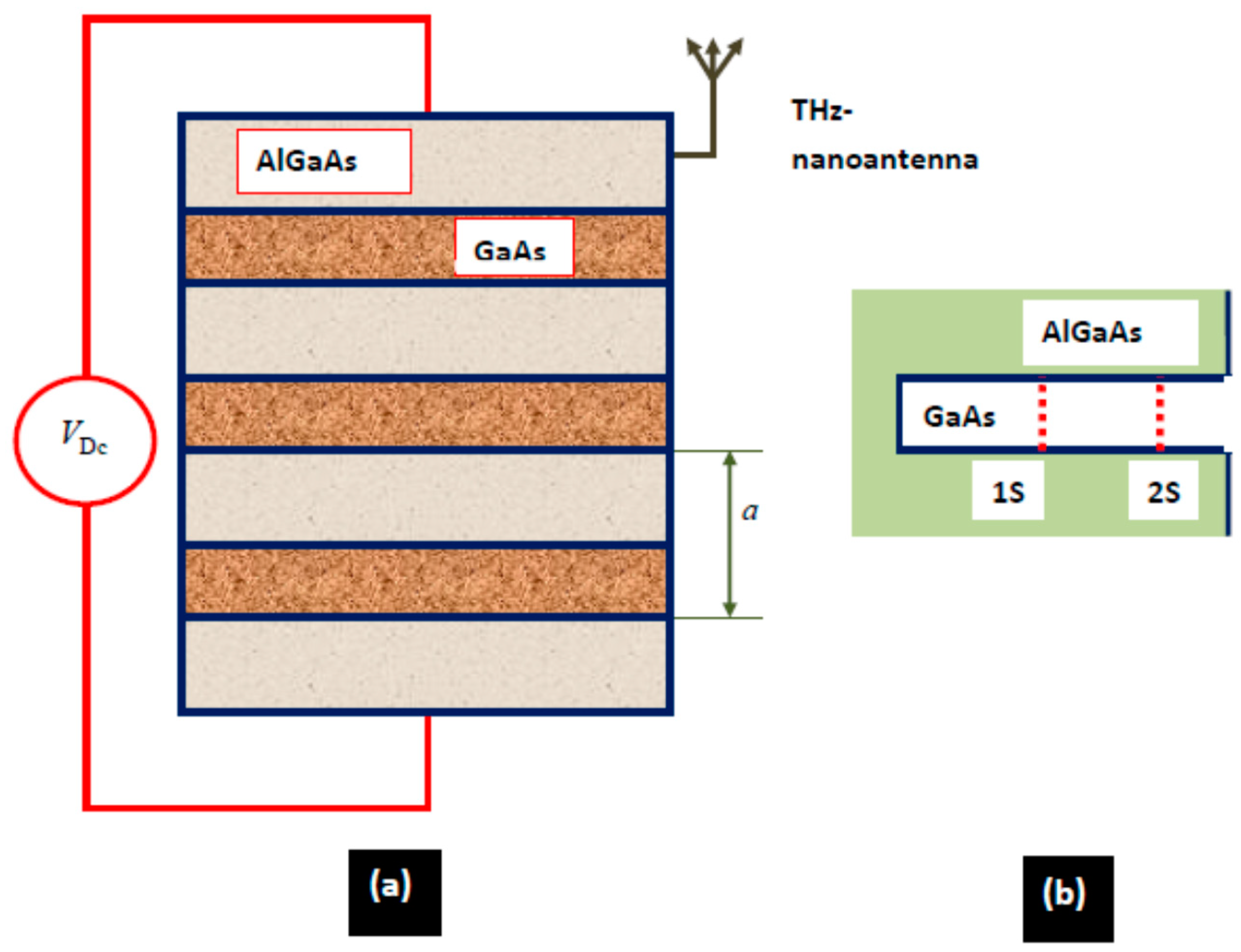
Figure 3.
Circuit diagram of a Josephson junction (crossed), which is inductively coupled with microwave resonator. The inductance describes the inductive environment of the junction. The inductance is a tool of control of the “junction-resonator” coupling (it is assumed ). Josephson energy strongly exceeds charging energy (). We model the resonator as an LC-circuit with effective inductance and effective capacitance . The single fluxonium plays role of atomic chain due to the interaction with inductive environment [53,54,55,56] (BO take place in the space of quasi-charge).

Figure 4.
Space-time distribution of inversion density. All frequencies are normalized to the frequency of quantum transition . Sampling Frequency = 4. The number of atoms N = 128, Rabi-frequency , electron initial Gaussian with , . (a) Light in the coherent state with . , . (b) Light in the coherent state with . , , . (c) light in vacuum. , , .
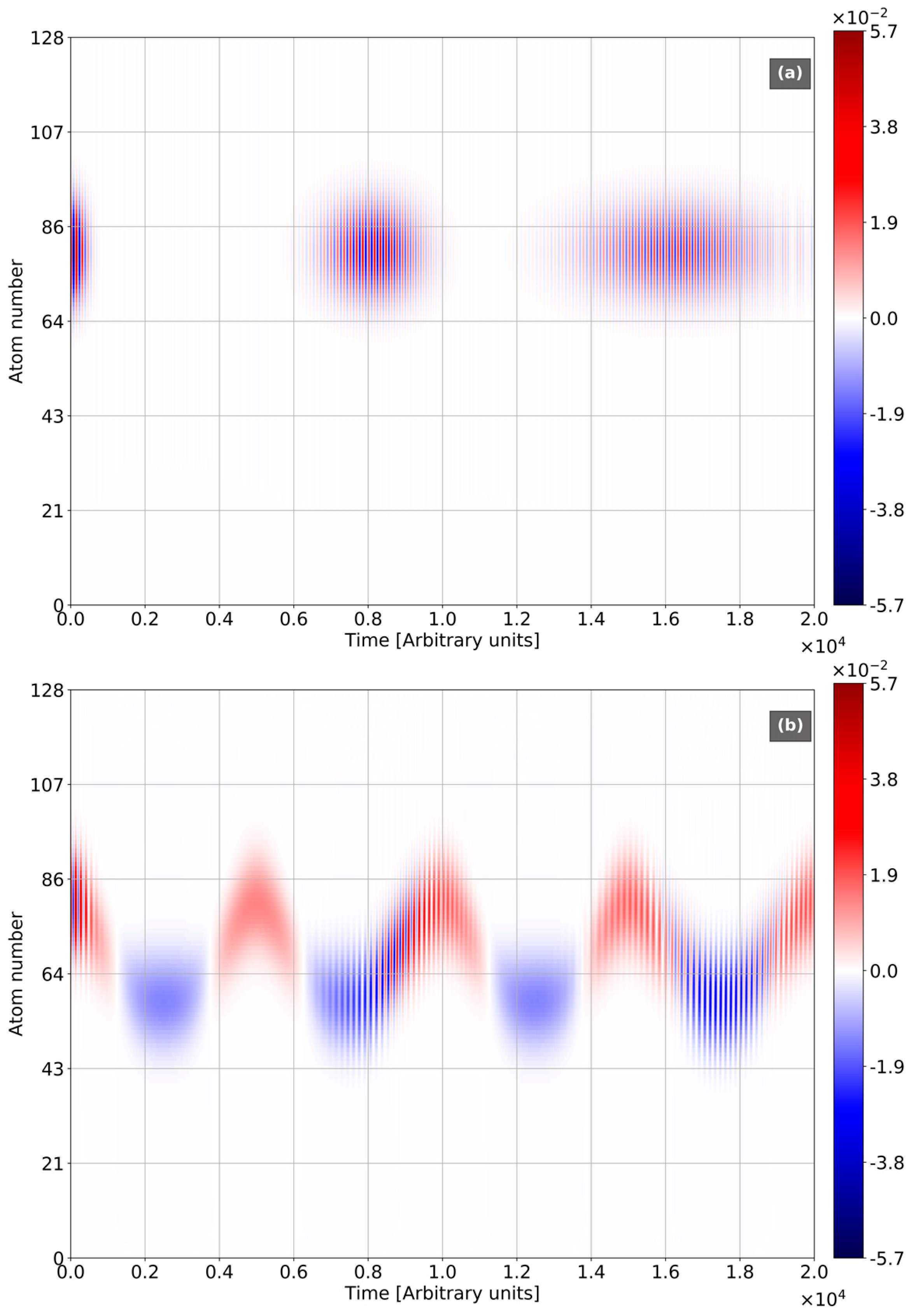

Figure 5.
Space-time distribution of tunnel current density. All frequencies are normalized to the frequency of quantum transition . Sampling Frequency = 4. The number of atoms N = 128, Rabi-frequency , electron initial Gaussian with , . (a) Light in the coherent state with . , . (b) Light in the coherent state with . , , . (c) Light in vacuum state. , , .

Figure 6.
Mean number of photons for light in the coherent state with . All frequencies are normalized to the frequency of quantum transition , . Sampling frequency = 4. (a) The chain with the number of atoms N = 128, , electron initial Gaussian with , , , . (b) Dressed single atom (Jaynes-Cummings model).
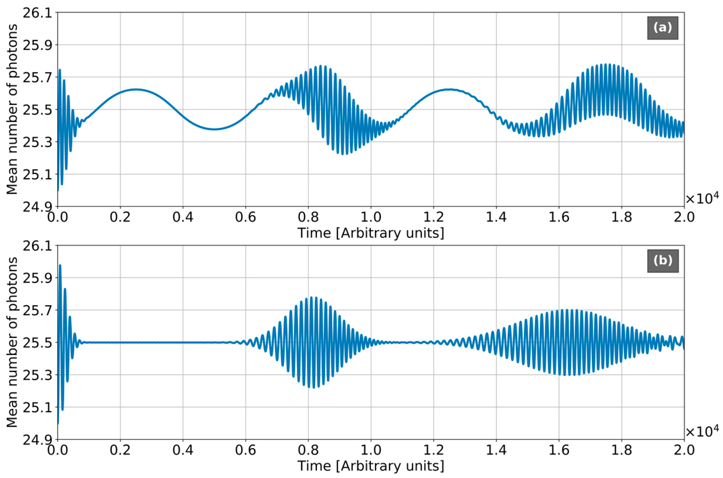
Figure 7.
Quantum-statistical characteristics of light in the vacuum state. All frequencies are normalized to the frequency of quantum transition , Sampling frequency = 4, Rabi-frequency , the chain with the number of atoms N = 128, , electron initial Gaussian with , , , . (a) Mean number of photons. (b) Photonic variance.

Figure 8.
Space-time distribution of inversion density for the case of atom-light initial entanglement. All frequencies are normalized to the frequency of quantum transition . Sampling frequency = 4. The number of atoms N = 128, Rabi-frequency , , electron initial Gaussian with , , , .
Figure 8.
Space-time distribution of inversion density for the case of atom-light initial entanglement. All frequencies are normalized to the frequency of quantum transition . Sampling frequency = 4. The number of atoms N = 128, Rabi-frequency , , electron initial Gaussian with , , , .

Figure 9.
Space-time distribution of tunnel current density for the case of atom-light initial entanglement. All frequencies are normalized to the frequency of quantum transition . Sampling frequency = 4. The number of atoms N = 128, Rabi-frequency , , electron initial Gaussian with , , , .
Figure 9.
Space-time distribution of tunnel current density for the case of atom-light initial entanglement. All frequencies are normalized to the frequency of quantum transition . Sampling frequency = 4. The number of atoms N = 128, Rabi-frequency , , electron initial Gaussian with , , , .

Figure 10.
Quantum-statistical characteristics of light in the entangled initial state. Mean number of photons for the case of atom-light initial entanglement. All frequencies are normalized to the frequency of quantum transition . Sampling Frequency = 4. Rabi-frequency , the chain with number of atoms N = 128, , electron initial Gaussian with , , , . (a) Mean number of photons. (b) Photonic variance.

Figure 11.
Space-time distribution of inversion density for pulse light in the coherent state with . All frequencies are normalized to the frequency of quantum transition . Sampling frequency=20. The number of atoms N = 128, Rabi-frequency , electron initial Gaussian with , , . Insert: the envelope of the light pulse in the time scale matched with the main picture.

Figure 12.
Space-time distribution of inversion density for pulse light in the coherent state with . All frequencies are normalized to the frequency of quantum transition . The number of atoms N = 128, Rabi-frequency , electron initial Gaussian with , , , , . Insert: the envelope of the light pulse in the time scale matched with the main picture.

© 2018 by the authors. Licensee MDPI, Basel, Switzerland. This article is an open access article distributed under the terms and conditions of the Creative Commons Attribution (CC BY) license (http://creativecommons.org/licenses/by/4.0/).
Share and Cite
MDPI and ACS Style
Levie, I.; Slepyan, G. Bloch Oscillations in the Chains of Artificial Atoms Dressed with Photons. Appl. Sci. 2018, 8, 937. https://doi.org/10.3390/app8060937
AMA Style
Levie I, Slepyan G. Bloch Oscillations in the Chains of Artificial Atoms Dressed with Photons. Applied Sciences. 2018; 8(6):937. https://doi.org/10.3390/app8060937
Chicago/Turabian StyleLevie, Ilay, and Gregory Slepyan. 2018. "Bloch Oscillations in the Chains of Artificial Atoms Dressed with Photons" Applied Sciences 8, no. 6: 937. https://doi.org/10.3390/app8060937
Note that from the first issue of 2016, this journal uses article numbers instead of page numbers. See further details here.