Probabilistic Ship Detection and Classification Using Deep Learning


School of Electrical and Electronic Engineering, Yonsei University, 50 Yonsei-ro, Seodaemun-gu, Seoul 03722, Korea
*
Author to whom correspondence should be addressed.
Appl. Sci. 2018, 8(6), 936; https://doi.org/10.3390/app8060936
Submission received: 9 April 2018
/
Revised: 15 May 2018
/
Accepted: 2 June 2018
/
Published: 5 June 2018
Abstract
:For an autonomous ship to navigate safely and avoid collisions with other ships, reliably detecting and classifying nearby ships under various maritime meteorological environments is essential. In this paper, a novel probabilistic ship detection and classification system based on deep learning is proposed. The proposed method aims to detect and classify nearby ships from a sequence of images. The method considers the confidence of a deep learning detector as a probability; the probabilities from the consecutive images are combined over time by Bayesian fusion. The proposed ship detection system involves three steps. In the first step, ships are detected in each image using Faster region-based convolutional neural network (Faster R-CNN). In the second step, the detected ships are gathered over time and the missed ships are recovered using the Intersection over Union of the bounding boxes between consecutive frames. In the third step, the probabilities from the Faster R-CNN are combined over time and the classes of the ships are determined by Bayesian fusion. To train and evaluate the proposed system, we collected thousands of ship images from Google image search and created our own ship dataset. The proposed method was tested with the collected videos and the mean average precision increased by 89.38 to 93.92% in experimental results.
1. Introduction
Accurate detection and reliable classification of nearby moving ships are essential functions of an autonomous ship, being closely linked to safe navigation [1,2]. When a ship navigates, the chance of collision with other ships is possible in various directions, such as those that overtake, approach head-on, or cross the autonomous ship. The International Regulations for Preventing Collisions at Sea (COLREGs) defines several rules to prevent collisions [3]. In particular, overtaking (rule 13), head-on (rule 14), and crossing (rule 15) situations are considered potential collision scenarios. Autonomous ships mainly collect information related to moving obstacles through non-visual sensors such as radar [4] and automatic identification systems (AIS) [5]. However, recognizing the nearby ships reliably is difficult if only using information collected from non-visual sensors to determine whether these are dangerous obstacles. Therefore, autonomous ships must recognize dangerous obstacles using a visual camera. This problem is similar to the detection of cars, pedestrians, lane, or traffic signs using a camera in autonomous vehicles.
Hitherto, some research concerning ship detection and classification has been reported. For example, seashore ship surveillance and ship detection from spaceborne optical images have been achieved [6,7,8,9]. Synthetic aperture radar (SAR) imagery was used to detect ships and objects on the surface of the earth [7,8]. Hwang et al. used artificial neural networks (ANN) for ship detection with X-band Kompsat-5 SAR imagery [9]. Unfortunately, most of the existing research focused only on ship detection based on spaceborne optical images, such as SAR imagery. Furthermore, these studies focused on visual ship detection based only on a single image. All previous works on ship detection and classification were based on a still image. To the best of our knowledge, no studies exist for the detection of ships using an image sequence or a video.
In this study, we propose a novel probabilistic ship detection and classification method using deep learning. This method considers the confidence from a deep learning detector as a probability and the probabilities from consecutive images are combined over time via Bayesian fusion. To the best of our knowledge, no research work has used the confidence from a deep learning detector in a Bayesian framework. The proposed ship detection system involves three steps. In the first step, ships are detected for each frame using Faster R-CNN [10]. In the second step, the detected ships are gathered over time and the missed ships are recovered using the Intersection over Union (IoU) of the bounding boxes between consecutive frames. The corresponding detection confidence is updated and the recovery compensates for the misdetection confidence over a few frames. This approach ensures robust ship detection and minimizes misdetection. In the third step, the probabilities from the Faster R-CNN are combined over time and the classes of the ships are determined by Bayesian fusion. The use of Bayesian fusion was supported by its reported use in prior studies [11,12].
To use a deep learning framework in ship detection, a ship dataset was needed to train the Faster R-CNN. Well-known image datasets, such as ImageNet [13], PASCAL visual object classes (VOC) challenge [14], and Microsoft common objects in context (MS COCO) [15], include ship images but the number of ship images is limited and the various classes of ships are not labeled. Popular intelligent transportation system (ITS) datasets, such as the Karlsruhe Institute of Technology and Toyota Technological Institute (KITTI) dataset [16], also does not include ship images. Because no public dataset exists for ship detection in the sea environment, we manually collected thousands of ship images from Google image search and built our own ship dataset.
The contributions of this paper can be summarized as follows. (1) This was the first attempt to detect and classify various classes of ships in a deep learning framework. (2) The confidence from a deep learning detector was considered as a probability and their values from the consecutive images were combined over time via Bayesian fusion. (3) Missed ships were recovered using the IoU of the bounding boxes between consecutive frames. (4) Large-scale ship detection dataset has been built by collecting ship images from google image search and annotating ground-truth bounding boxes.
The remainder of this paper is organized as follows: in Section 2, the background for the Faster R-CNN and the basic idea underlying this paper are outlined. In Section 3 and Section 4, the details about the proposed method are explained. In Section 5, the experimental results, performance, and discussion are presented. Finally, the conclusions drawn from this study are presented in Section 6.
2. Ship Detection and Classification from an Image
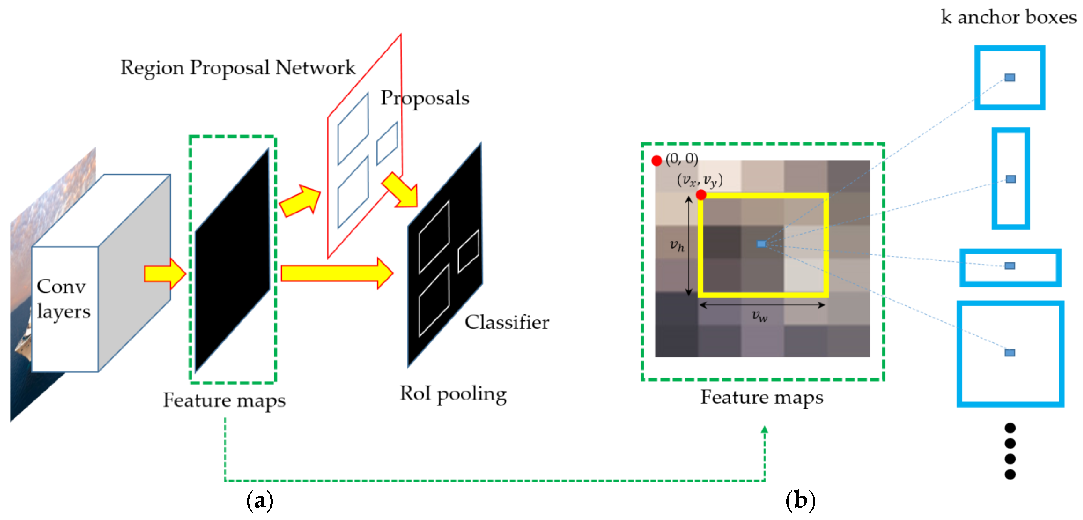
In this study, ships were detected in each frame using Faster R-CNN [10], as in our previous work [17]. The Faster R-CNN is a representative region-based object detection model based on deep learning. As shown by Huang et al. [18], Faster R-CNN outperforms the other models [19,20] in general object detection problem. Although R-CNN [21] and the Fast R-CNN [22] use Selective Search [23] to generate possible object locations, Faster R-CNN introduced the region proposal network (RPN), which outputs region proposals from shared full-image convolutional features, thereby improving speed performance. Faster R-CNN combines RPN and Fast R-CNN into a single network for object detection by sharing their convolutional features, as shown in Figure 1.
When an image is used as input data, the convolutional neural network (CNN) generates the convolutional features. Then, the fully-convolutional RPN predicts the bounding box and object scores at each position of the convolutional features, as shown in Figure 1b. Thus, the RPN tells the Fast R-CNN where to look and classify. In our experiments, we used the Zeiler and Fergus model (ZF net) [24] that five shareable convolutional layers.
The Faster R-CNN is trained with a four-step training algorithm to learn shared features via alternative optimization. In the first step, the RPN is initialized with a pre-trained model and then fine-tuned end-to-end to propose regions. In the second step, the Fast R-CNN is trained using the region proposals generated by the first-step RPN not sharing convolutional layers. In the third step, the shared convolutional layers are fixed and the unique layers of RPN are fine-tuned. Finally, the layers unique to Fast R-CNN are fine-tuned while maintaining the shared convolutional layers. The detailed alternating algorithm for training the Faster R-CNN is found in Ren et al. [10].
The Faster R-CNN detection result for a single image can be expressed as a bounding box represented by:
where denotes the four values of the bounding box: coordinates (,), width (), and height (), as shown in Figure 1b. The class confidence of the bounding box predicted by the Faster R-CNN can be represented by:
where denotes the class of ship, is one of the possible values that can take, is the bounding box predicted by the Faster R-CNN, and is the number of classes in the ship dataset created in this study.
We used seven different classes of ships in this study; thus, was set to eight, including the background. The class index is summarized in Table 1. The class of the detected bounding box is predicted by:
As shown in Equation (3), the determined class of the predicted bounding box is the class with the highest confidence. Our method considers the class and detection confidence from the Faster R-CNN as the probability and exploits it using Bayesian fusion.
3. Building a Sequence of Bounding Boxes
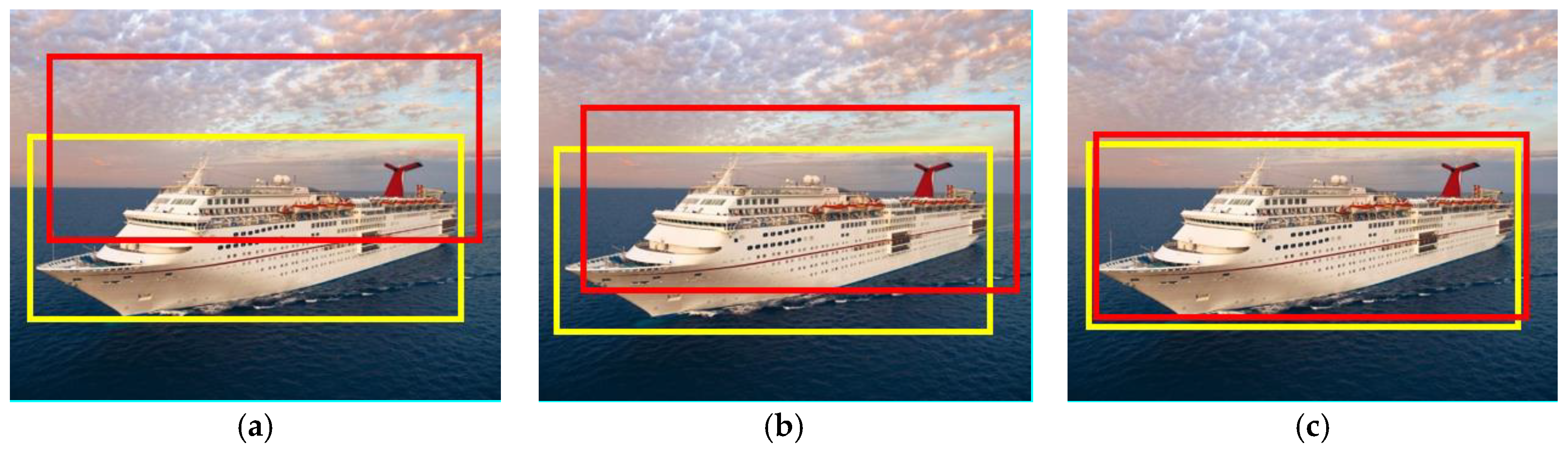
In this section, we build a sequence for the bounding boxes using the boxes returned from the Faster R-CNN over time. In building the bounding box sequence, two practical issues had to be considered. The first issue was which bounding box to select at each time to create a reasonable sequence. The second issue involved how to handle the situation in which all the bounding boxes at time did not make sense and when the target ship has apparently not been detected. To address these issues, we used the intersection over union (IoU) of the target bounding box and the predicted bounding boxes. Figure 2 illustrates two bounding boxes with IoU of 0.3, 0.4, and 0.9. For the two given bounding boxes and , IoU computes the intersection of two boxes divided by the area of their union as follows:
Concerning the first issue, we assumed that the target ships do not move rapidly at sea. Therefore, when the Faster R-CNN returns bounding boxes from a given image in the tth frame, the bounding box with the largest IoU with the bounding box in the previous frame is used as the bounding box in the current frame:
where denotes the rth predicted bounding boxes returned by Faster R-CNN in the tth frame.
Concerning the second issue, when the detector in the current frame did not predict the position of the ship correctly and , the target ship is likely to be missed. In this case, we enlarged slightly from by adding an offset to avoid missing ship detection, where denotes a threshold. This can be represented by:
where denotes an offset added to the bounding box. Figure 3 shows the update of the target ship-bounding box based on IoU.
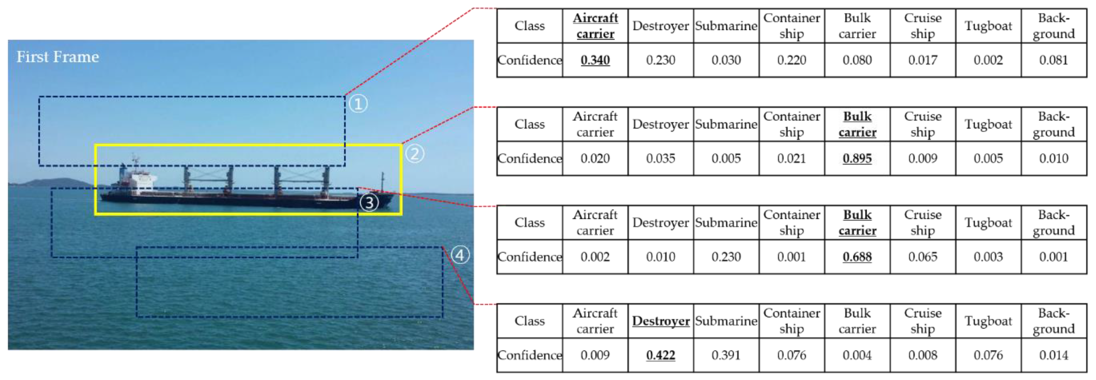
If bounding boxes are predicted in the first frame, the initial bounding box was selected as the one with the highest detection confidence busing:
For example, Faster R-CNN predicts four bounding boxes with class confidence in the first frame, as shown in Figure 4. Since the determined class of the predicted bounding box is the class with the highest confidence, the classes of the detected boxes from ① to ④ are an aircraft carrier (0.34), bulk carrier (0.895), bulk carrier (0.668), and a destroyer (0.422), respectively. In this case, from Equation (7), we selected bounding box ② as the initial bounding box in the video.
4. Probabilistic Ship Detection and Classification in a Sequence of Images
In this section, is a sequence of the bounding boxes predicted by the Faster R-CNN, where is the bounding box detected at time . We determine the class of the bounding box sequence using maximum a posteriori (MAP). That is, the class of the sequence of the bounding boxes is predicted by:
Assuming that denotes the current time, we can rewrite Equation (8) as:
where is divided into the current measurement and all the previous measurements are . Using the Bayes rule, Equation (9) can be rewritten as:
Since the current measurement is not affected by previous measurements conditioned on , we obtain , and Equation (10) can be simplified as:
Substituting the Bayes rule
into Equation (11) yields:
Furthermore, we define the class confidence of a sequence of bounding boxes from the Faster R-CNN with:
and consider a new quantity:
Substituting Equation (13) into Equation (15) yields:
Herein, we denote the detection confidence for the bounding box selected in Equation (5) as:
For practical consideration, if the detector missed the target ship, we considered the recovered bounding box in Equation (6) as a background; then, its detection confidence is assigned by:
Then, substituting Equation (17) into Equation (16) yields:
where is the previous confidence of the sequence at time , is the initial confidence, and is the confidence of the tth frame of .
If we define
then, we can obtain the following from Equation (19):
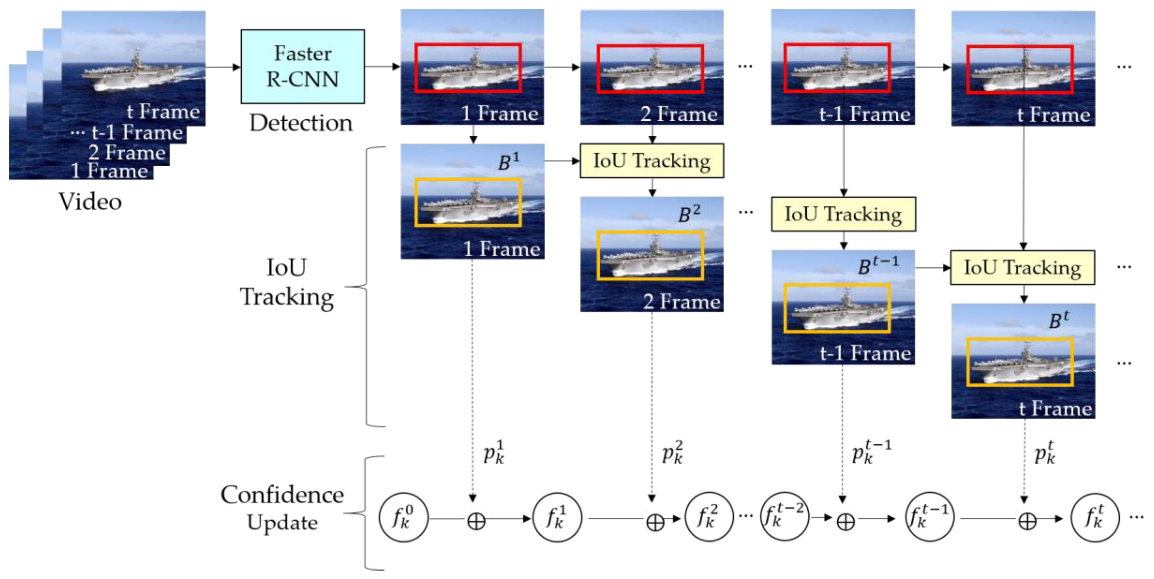
From Equations (19) and (20), we can update the sequence confidence at time from the previous sequence confidence at time , and the current frame confidence from the Faster R-CNN at time . Thus, we did not need to retain all the previous frame confidences to compute the current sequence confidence. Then, we can predict the class of a sequence from Equation (8). In this study, we set the IoU threshold to 0.5 and to (−1, −1, 1, 1). Summarizing the abovementioned results, the proposed probabilistic ship detection algorithm using video is outlined in Algorithm 1 and illustrated in Figure 5.
| Algorithm 1: Probabilistic ship detection and classification from video. | |
| Step 1: | At frame 1, initialize the target ship-bounding box |
| Step 2: | For a given image at frame update the bounding boxes |
| If , | |
| else | |
| End | |
| Step 3: | Evaluate the class confidence of a sequence of bounding boxes recursively by |
| Step 4: | Determine the class at frame using |
| Step 5: | For every next frame, repeat Steps 2, 3, and 4. |
5. Experimental Results
We built our own ship dataset to train the Faster R-CNN and evaluate the proposed method. For this dataset, 7000 ship images were collected by Google image search and they were manually labeled as one of seven classes: aircraft carrier, destroyer, submarine, container ship, bulk carrier, cruise ship, and tugboat.
5.1. Ship Dataset
The dataset mainly focused on large ships, which were divided into two types navigating in the ocean: warship and merchant ship. Three warship classes exist: aircraft carrier, destroyer, and submarine. Three classes of merchant also exist: container ship, bulk carrier, and cruise ship. Finally, we included a small ship in the dataset, a tugboat that assists large ships in entering and leaving a port, resulting in seven classes.
To train the Faster R-CNN for ship detection and evaluate single image detection, a total of 7000 still images were collected. Each class included 1000 images, completely balancing the problem. All the still images were manually gathered from Google image search. Most of the collected still images were completely different from and separated from other collected images and none were not consecutive. The ship image dataset was divided into a training dataset and a test dataset, as summarized in Table 2. In detail, 5250 images (75%, 750 images per class) among the 7000 images were used for the training the Faster R-CNN, and 1750 images (25%, 250 images per class) were used to test single image detection.
To evaluate ship detection performance on videos, seven video clips involving all the aforementioned classes were downloaded from YouTube in MPEG-4 video format. A test video file was decomposed into a sequence of still images that were consecutive in time and each image was processed by Faster R-CNN. The detection result of each image was combined with that of the consecutive images and the combined result was used in video simulation.
5.2. Performance
5.2.1. Results of the Single Image Detection
The same hyper parameters used in the original Faster R-CNN [10] were applied to train our Faster R-CNN for ship detection. The hyper parameters used in our experiments were as follows: learning rate: 0.001, momentum: 0.9, and weight decay, 0.0005. The ZF net pre-trained on ImageNet was used as a base CNN to extract features and fine-tune the network using our ship dataset. The maximum iteration was set to 10,000. We use the Caffe [25] framework to train the Faster R-CNN on Ubuntu 16.04 LTS and NVIDIA GeForce GTX 980 on GPU. Table 3 shows the results of the ship detection using the Faster R-CNN fine-tuned by the above training set. The results of the ship detection using the Faster R-CNN by the test sample images are shown in Figure 6.
5.2.2. Results of Detection Based on Video
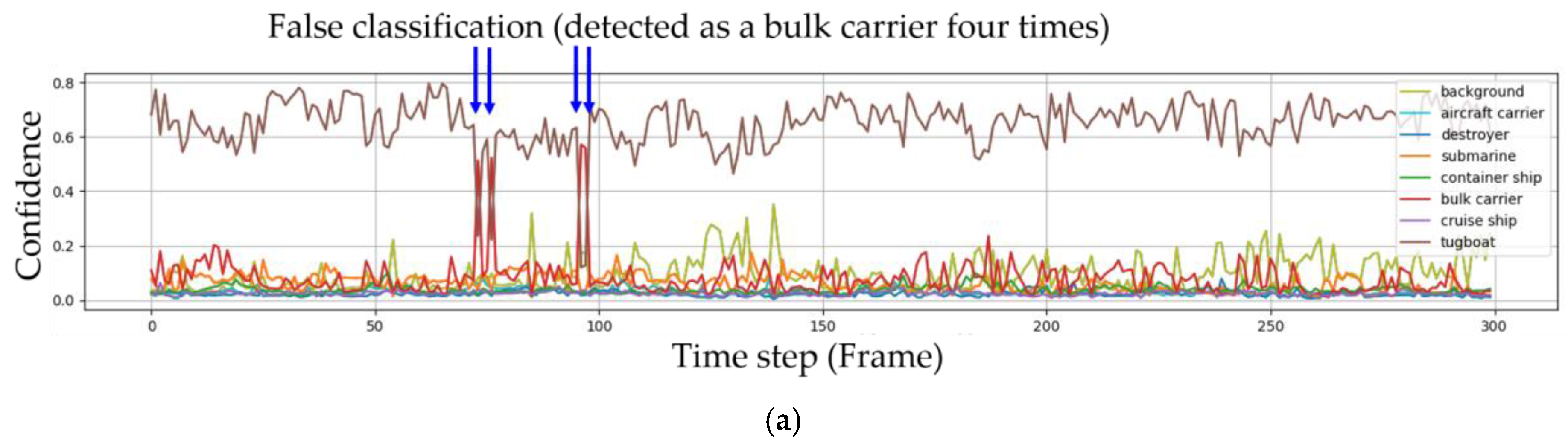
Seven sequences of images were used to demonstrate the performance of the proposed method based on video. Among them, two videos were considered in detail. In the first sequence involving a tugboat, the weather was relatively fine and the ships were not influenced by environmental factors. In the second sequence involving a destroyer, however, the weather was windy and the environmental factors, such as waves and wind, influence ships. The Faster R-CNN returned eight confidences, one for each class, and the eight confidences equaled 1 in each frame, as shown in Equation (17). In Figure 7, the changes in the eight confidences are plotted against the frames for the first sequence. The subfigures in the first, second and third rows correspond to the Faster R-CNN; Faster R-CNN and IoU tracking; and Faster R-CNN, IoU tracking and Bayesian fusion, respectively.
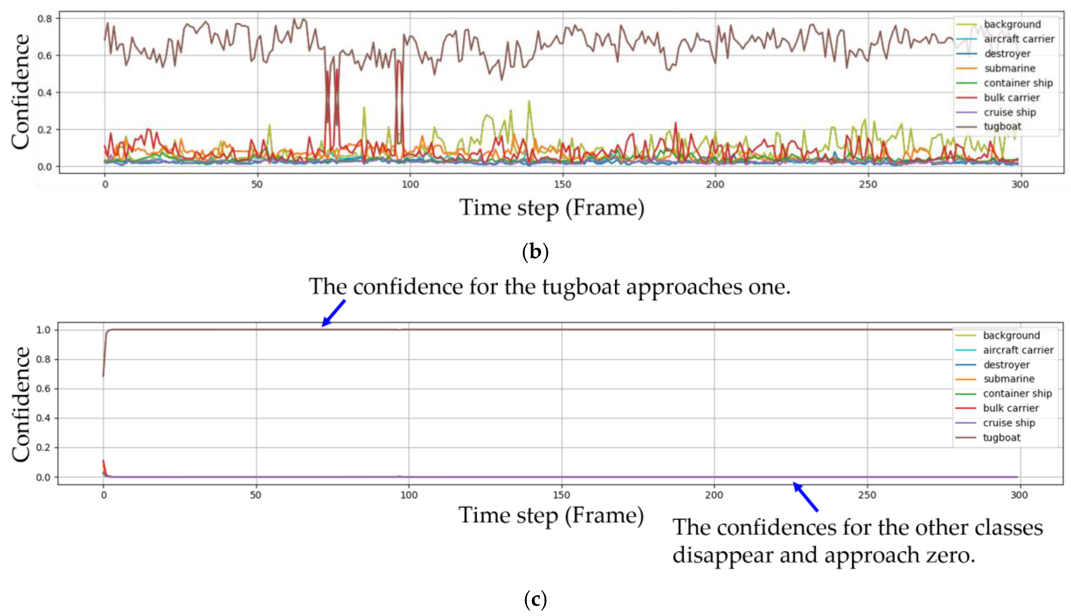
The confidence in Figure 7a implies and the confidence in Figure 7c implies . In the first sequence, the target ship is a tugboat. In Figure 7a, the tugboat is classified as a bulk carrier four times by Faster R-CNN. The confidence of the tugboat also does not remain steady but changes irregularly. In Figure 7b, IoU tracking is also used with the Faster R-CNN. When the target was not detected or the IoU was lower than the threshold, the bounding box was considered background and the corresponding confidences were assigned by Equation (18). However, in the figure, no background confidence was observed since all the targets in each frame were detected by the Faster R-CNN and the IoU values from IoU tracking were higher than the threshold. Figure 7c shows the experimental result when Faster R-CNN, IoU tracking and Bayesian fusion were used together. The confidence for the tugboat was steady and approached one after a few frames, and the confidences for the other classes disappeared and approached zero.
The experimental results for the second sequence are shown in Figure 8. Unlike the first sequence, the ships were affected by environmental factors. The target ship in the second sequence was a destroyer. Similar to Figure 7, the change in the eight confidences is plotted against frames for the second sequence in Figure 8. The subfigures in the first, second and third rows in Figure 8 correspond to Faster R-CNN; Faster R-CNN and IoU tracking; and Faster R-CNN, IoU tracking and Bayesian fusion, respectively.
First, let us consider Intervals 1 and 4 in Figure 8. In the two intervals, the destroyer was falsely classified as an aircraft carrier, as shown in Figure 8a,b. In particular, the target ship was classified not as a destroyer but as an aircraft carrier in six frames in a row from frame 235 to 240. However, the proposed method overcame the false classification problem and the confidence for the destroyer progressed steadily to one, as shown in Figure 8c. Second, consider Interval 2. In this interval, the destroyer was not detected and was actually classified as background by the IoU tracking several times. However, the proposed method again overcame the misdetections again and the confidence for a destroyer progressed steadily to one, as shown in Figure 8c. Third, consider Interval 3, which was slightly different from Intervals 1, 2 and 4. Unlike the previous intervals, several misdetections and tens of false classifications occurred together in Interval 3. The proposed method worked well even for this challenging situation for the first 30 frames but the frequency of the misdetection and false classification exceeded a certain threshold. Moreover, our algorithm failed to classify effectively and returned the wrong result.
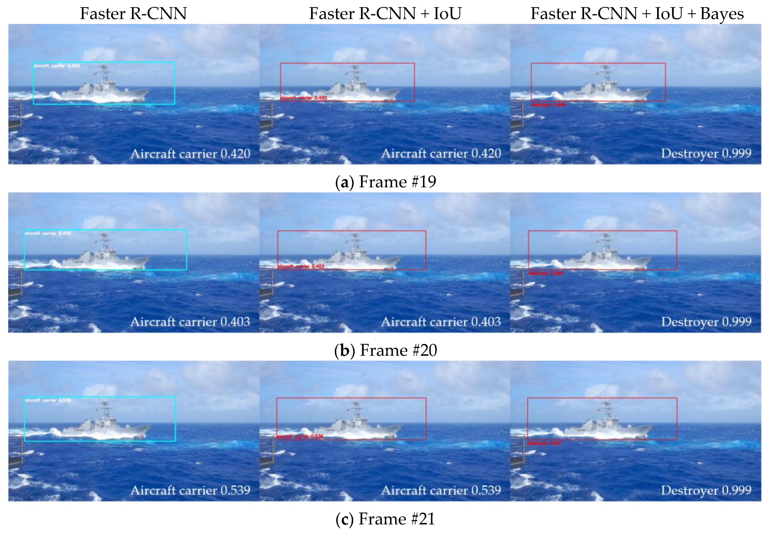
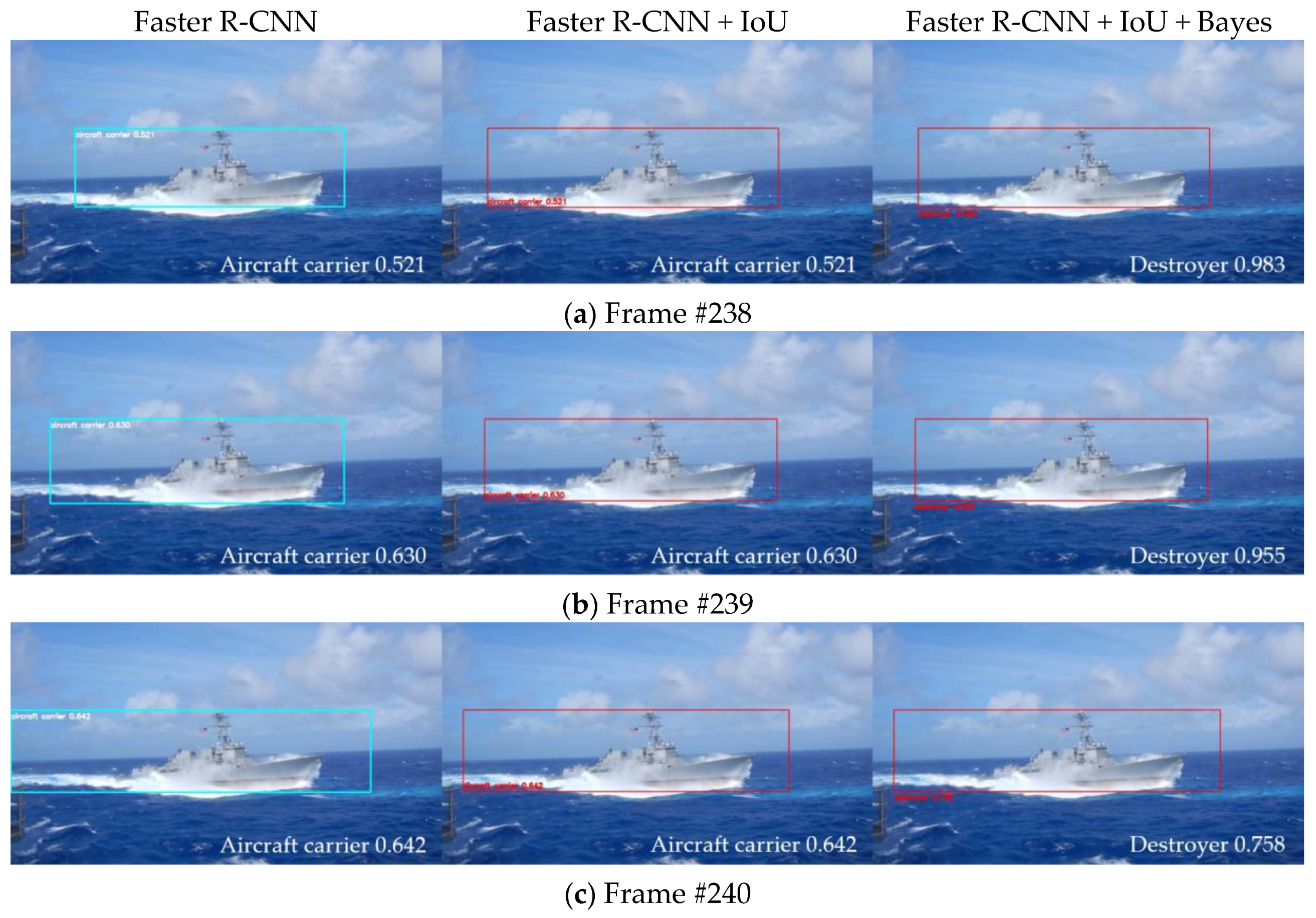
Three competing methods are compared on a per-frame basis in Table 4. As stated, the ground truth was a destroyer. In Intervals 1 and 4, only Faster R-CNN returned a false classification for the aircraft carrier in several frames such as #19, #20 and #21 and its confidence remained around 0.5. When Faster R-CNN was combined with IoU tracking and Bayesian fusion, however, the confidence steadily increased and approached one. In Interval 2, only Faster R-CNN often missed the destroyer but when it was combined with IoU tracking and Bayesian fusion, Faster R-CNN overcame the misdetections and the confidence also approached one. Here, when the target was not detected or falsely classified for several consecutive frames, for example, during frames #124 to #127 in Interval 2 frame or frames #235 to #240 in Interval 4, the confidence for the destroyer dropped to around 0.9. However, the confidence quickly recovered from the loss when Faster R-CNN returned the correct result. Figure 9, Figure 10 and Figure 11 show captured images from the frames #19 to #21 in Interval 1, frames #125 to #127 in Interval 2 and frames #238 to #240 in interval 4, respectively.
The performance of ship detection with the proposed method on test videos was compared with using only Faster R-CNN for ship detection. The ship detection results are summarized in Table 5. Overall, our proposed method outperformed the previous Faster R-CNN detector.
6. Conclusions
In this study, a probabilistic ship detection and classification system for video using deep learning was proposed. To train the detector and evaluate the proposed system, we collected thousands of ship images from a Google image search and built our own ship dataset. The probabilistic ship detection and classification system demonstrated better detection and classification performance compared to when only Faster R-CNN was used. The proposed method used IoU tracking to build a sequence of the bounding boxes and considered the confidence from the detector as a probability. The undetected ships were recovered by IoU tracking. Moreover, the probabilities of the detection accumulated over time and the classes of the ships were determined by Bayesian fusion. In the experiments, the proposed method was tested with two sequences of images and showed considerable improvement in both detection and classification over prior methods.
Author Contributions
K.K., S.H. and E.K. designed the algorithm, and carried out the experiment, analyzed the result and wrote the paper; B.C. analyzed the data and gave helpful suggestion on this research.
Acknowledgments
This work was supported by the Basic Science Research Program through the National Research Foundation of Korea (NRF) funded by the Ministry of Education, Science and Technology under Grant NRF-2016R1A2A2A05005301.
Conflicts of Interest
The authors declare no conflict of interest.
References
- Statheros, T.; Howells, G.; Maier, K.M. Autonomous ship collision avoidance navigation concepts, technologies and techniques. J. Navig. 2008, 61, 129–142. [Google Scholar] [CrossRef]
- Sun, X.; Wang, G.; Fan, Y.; Mu, D.; Qiu, B. An Automatic Navigation System for Unmanned Surface Vehicles in Realistic Sea Environments. Appl. Sci. 2018, 8, 193. [Google Scholar] [Green Version]
- International Maritime Organization (IMO). Available online: http://www.imo.org/en/About/Conventions/-ListOfConventions/Pages/COLREG.aspx (accessed on 3 April 2018).
- Liu, Z.; Zhang, Y.; Yu, X.; Yuan, C. Unmanned surface vehicles: An overview of developments and challenges. Annu. Rev. Control 2016, 41, 71–93. [Google Scholar] [CrossRef]
- Stitt, I.P.A. AIS and collision avoidance—A sense of déjà vu. J. Navig. 2004, 57, 167–180. [Google Scholar] [CrossRef]
- Tang, J.; Deng, C.; Huang, G.B.; Zhao, B. Compressed-domain ship detection on spaceborne optical image using deep neural network and extreme learning machine. IEEE Trans. Geosci. Remote Sens. 2015, 53, 1174–1185. [Google Scholar] [CrossRef]
- Crisp, D.J. The State-of-the-Art in Ship Detection in Synthetic Aperture Radar Imagery; No. DSTO-RR-0272; Defence Science and Technology Organisation Salisbury (Australia) Info Sciences Lab: Canberra, Australia, 2004. [Google Scholar]
- Migliaccio, M.; Nunziata, F.; Montuori, A.; Brown, C.E. Marine added-value products using RADARSAT-2 fine quad-polarization. Can. J. Remote Sens. 2012, 37, 443–451. [Google Scholar] [CrossRef]
- Hwang, J.I.; Chae, S.H.; Kim, D.; Jung, H.S. Application of Artificial Neural Networks to Ship Detection from X-Band Kompsat-5 Imagery. Appl. Sci. 2017, 7, 961. [Google Scholar] [CrossRef]
- Ren, S.; He, K.; Girshick, R.; Sun, J. Faster R-CNN: Towards real-time object detection with region proposal networks. In Advances in Neural Information Processing Systems (NIPS), Proceedings of the NIPS 2015, Montréal, Canada, 7–12 December 2015; NIPS Foundation, Inc.: La Jolla, CA, USA, 2015; pp. 91–99. [Google Scholar]
- Park, S.; Hwang, J.P.; Kim, E.; Lee, H.; Jung, H.G. A neural network approach to target classification for active safety system using microwave radar. Expert Syst. Appl. 2010, 37, 2340–2346. [Google Scholar] [CrossRef]
- Hong, S.; Lee, H.; Kim, E. Probabilistic gait modelling and recognition. IET Comput. Vis. 2013, 7, 56–70. [Google Scholar] [CrossRef]
- Russakovsky, O.; Deng, J.; Su, H.; Krause, J.; Satheesh, S.; Ma, S.; Huang, Z.; Karpathy, A.; Khosla, A.; Berg, A.C.; et al. Imagenet large scale visual recognition challenge. Int. J. Comput. Vis. 2015, 115, 211–252. [Google Scholar] [CrossRef]
- Everingham, M.; Van Gool, L.; Williams, C.K.; Winn, J.; Zisserman, A. The pascal visual object classes (VOC) challenge. Int. J. Comput. Vis. 2010, 88, 303–338. [Google Scholar] [CrossRef]
- Lin, T.Y.; Maire, M.; Belongie, S.; Hays, J.; Perona, P.; Ramanan, D.; Dollár, P.; Zitnick, C.L. Microsoft COCO: Common Objects in Context. In Proceedings of the European Conference on Computer Vision (ECCV) 2014, Zurich, Switzerland, 6–12 September 2014; Springer: Cham, Switzerland, 2014; pp. 740–755. [Google Scholar]
- Geiger, A.; Lenz, P.; Urtasun, R. Are We Ready for Autonomous Driving? The KITTI Vision Benchmark Suite. In Proceedings of the 2012 IEEE Conference on Computer Vision and Pattern Recognition (CVPR), Providence, RI, USA, 16–21 June 2012; pp. 3354–3361. [Google Scholar]
- Kim, K.H.; Hong, S.J.; Choi, B.H.; Kim, I.H.; Kim, E.T. Ship Detection Using Faster R-CNN in Maritime Scenarios. In Proceedings of the Conference on Information and Control Systems (CICS) 2017, Dubal, United Arab Emirates, 29–30 April 2017; pp. 158–159. (In Korean). [Google Scholar]
- Huang, J.; Rathod, V.; Sun, C.; Zhu, M.; Korattikara, A.; Fathi, A.; Fischer, I.; Wojna, Z.; Song, Y.; Murphy, K.; et al. Speed/Accuracy Trade-Offs for Modern Convolutional Object Detectors. In Proceedings of the IEEE 2017 Conference on Computer Vision and Pattern Recognition (CVPR) 2017, Honolulu, HI, USA, 21–26 July 2017; pp. 7310–7311. [Google Scholar]
- Dai, J.; Li, Y.; He, K.; Sun, J. R-FCN: Object detection via region-based fully convolutional networks. In Advances in Neural Information Processing Systems (NIPS), Proceedings of the NIPS 2016 Barcelona, Spain, 5–10 December 2016; NIPS Foundation, Inc.: La Jolla, CA, USA, 2016; pp. 379–387. [Google Scholar]
- Liu, W.; Anguelov, D.; Erhan, D.; Szegedy, C.; Reed, S.; Fu, C.Y.; Berg, A.C. SSD: Single shot multiBox Detector. In Proceedings of the European Conference on Computer Vision (ECCV) 2016, Amsterdam, The Netherlands, 8–16 October 2016; Springer: Cham, Switzerland, 2016; pp. 21–37. [Google Scholar]
- Girshick, R.; Donahue, J.; Darrell, T.; Malik, J. Rich Feature Hierarchies for Accurate Object Detection and Semantic Segmentation. In Proceedings of the IEEE 2014 Conference on Computer Vision and Pattern Recognition (CVPR), Columbus, OH, USA, 23–28 June 2014; pp. 580–587. [Google Scholar]
- Girshick, R. Fast R-CNN. In Proceedings of the IEEE 2015 Conference on Computer Vision and Pattern Recognition (CVPR), Boston, MA, USA, 7–12 June 2015; pp. 1440–1448. [Google Scholar]
- Uijlings, J.R.; Van De Sande, K.E.; Gevers, T.; Smeulders, A.W. Selective search for object recognition. Int. J. Comput. Vis. 2013, 104, 154–171. [Google Scholar] [CrossRef]
- Zeiler, M.D.; Fergus, R. Visualizing and understanding convolutional networks. In Proceedings of the European Conference on Computer Vision (ECCV), Zurich, Switzerland, 6–12 September 2014; Springer: Cham, Switzerland; pp. 818–833. [Google Scholar]
- Jia, Y.; Shelhamer, E.; Donahue, J.; Karayev, S.; Long, J.; Girshick, R.; Guadarrama, S.; Darrell, T. Caffe: Convolutional architecture for fast feature embedding. In Proceedings of the 22nd ACM International Conference on Multimedia, Orlando, FL, USA, 3–7 November 2014; pp. 675–678. [Google Scholar]
Figure 1.
Structures of (a) Faster region-based convolution neural network (Faster R-CNN) and (b) region proposal network (RPN).
Figure 1.
Structures of (a) Faster region-based convolution neural network (Faster R-CNN) and (b) region proposal network (RPN).

Figure 2.
An illustration of two bounding boxes with an Intersection over Union (IoU) of (a) 0.3, (b) 0.5, and (c) 0.9.
Figure 2.
An illustration of two bounding boxes with an Intersection over Union (IoU) of (a) 0.3, (b) 0.5, and (c) 0.9.

Figure 3.
IoU tracking. (a) IoU is equal to or larger than the threshold and (b) IoU is less than the threshold. If IoU is less than the threshold, the bounding box in frame increases slightly and is updated as the target ship-bounding box to avoid missing ship detection.
Figure 3.
IoU tracking. (a) IoU is equal to or larger than the threshold and (b) IoU is less than the threshold. If IoU is less than the threshold, the bounding box in frame increases slightly and is updated as the target ship-bounding box to avoid missing ship detection.
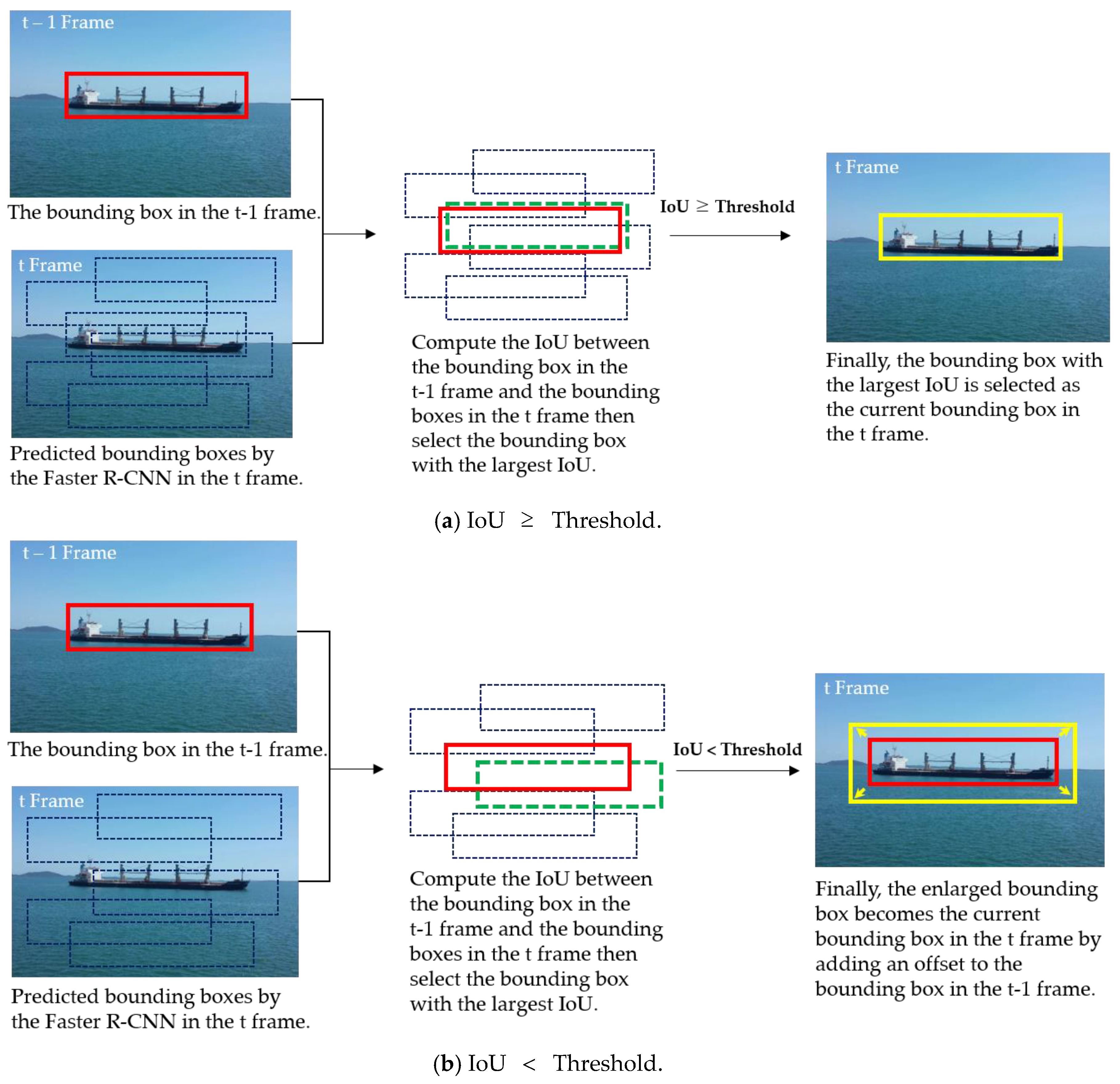
Figure 4.
Initial bounding box selection in the first frame.

Figure 5.
Robust single ship detection system based on video in our proposed algorithm.

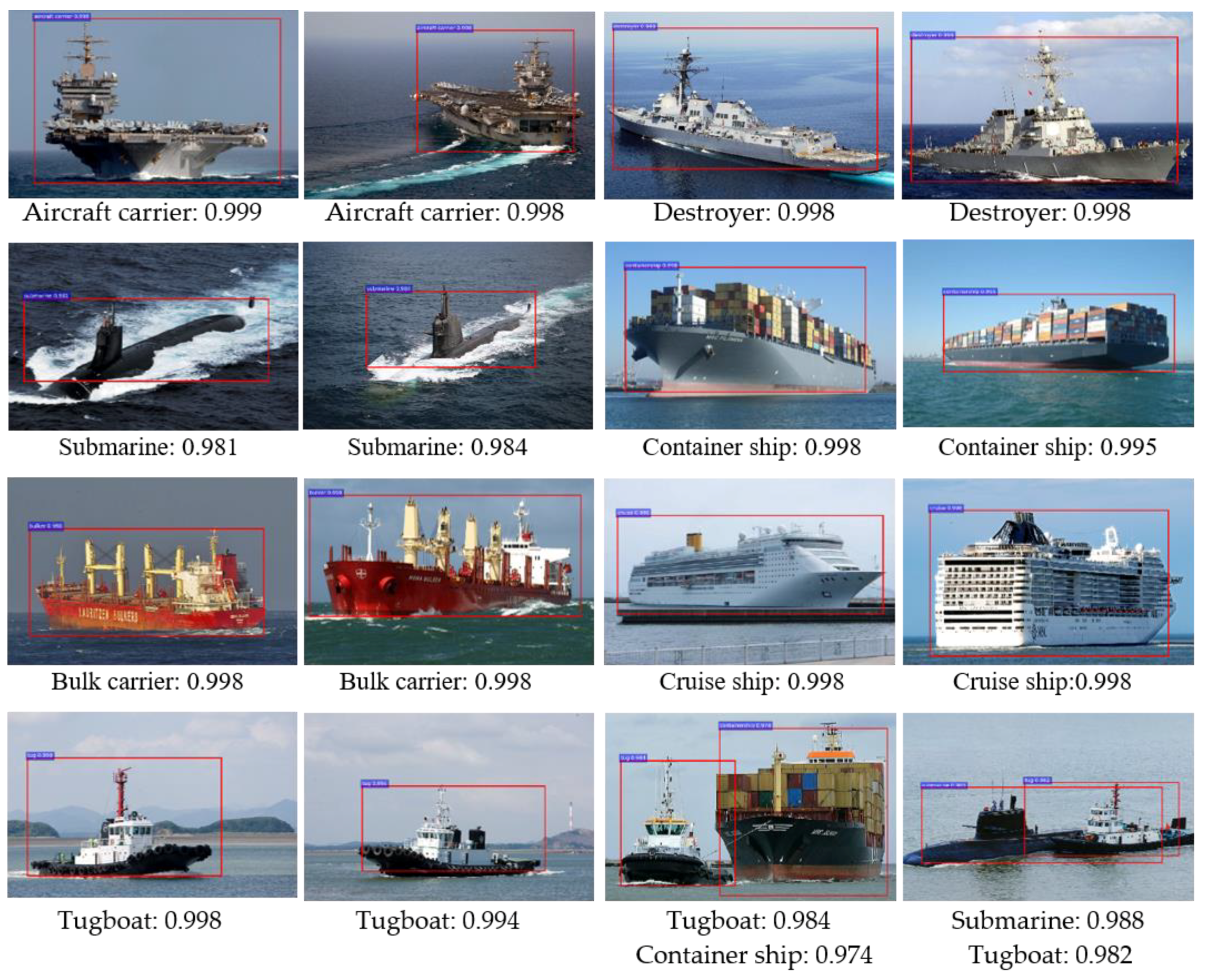
Figure 6.
Results of the ship detection using the Faster R-CNN based on the test images.

Figure 7.
The change of confidences in the image sequence without environmental factors. (a) Faster R-CNN, (b) Faster R-CNN and IoU tracking, and (c) Faster R-CNN, IoU tracking, and Bayesian fusion.
Figure 7.
The change of confidences in the image sequence without environmental factors. (a) Faster R-CNN, (b) Faster R-CNN and IoU tracking, and (c) Faster R-CNN, IoU tracking, and Bayesian fusion.


Figure 8.
The change in the confidences in the image sequence with environmental factors: (a) Faster R-CNN, (b) Faster R-CNN and IoU tracking, and (c) Faster R-CNN, IoU tracking and Bayesian fusion.
Figure 8.
The change in the confidences in the image sequence with environmental factors: (a) Faster R-CNN, (b) Faster R-CNN and IoU tracking, and (c) Faster R-CNN, IoU tracking and Bayesian fusion.
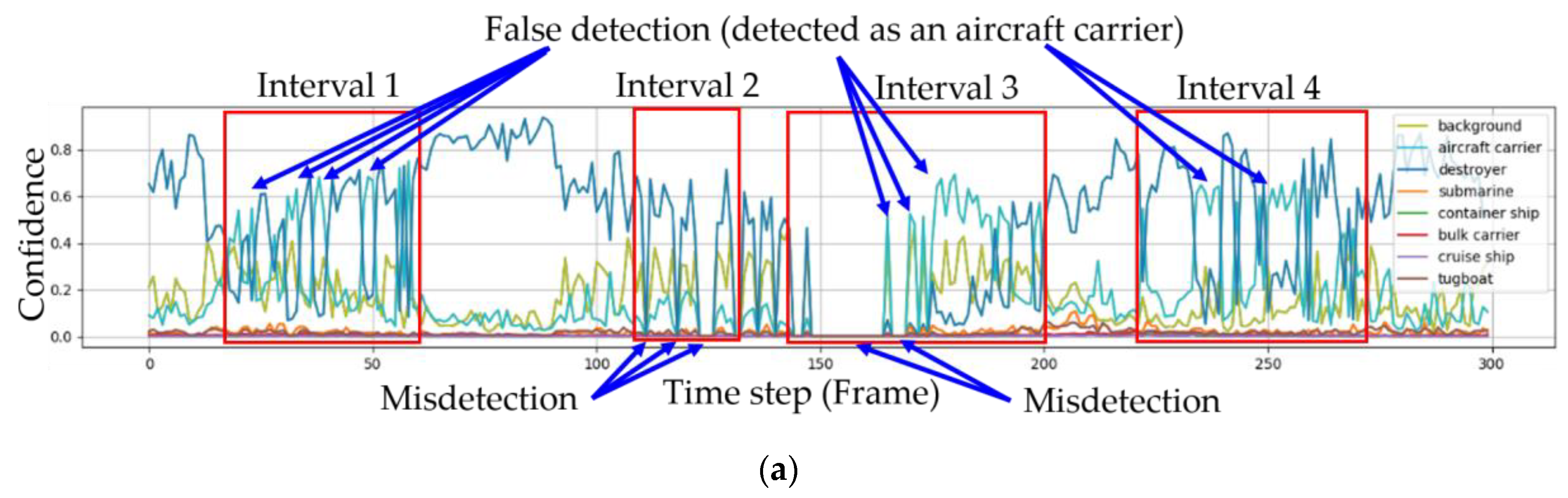
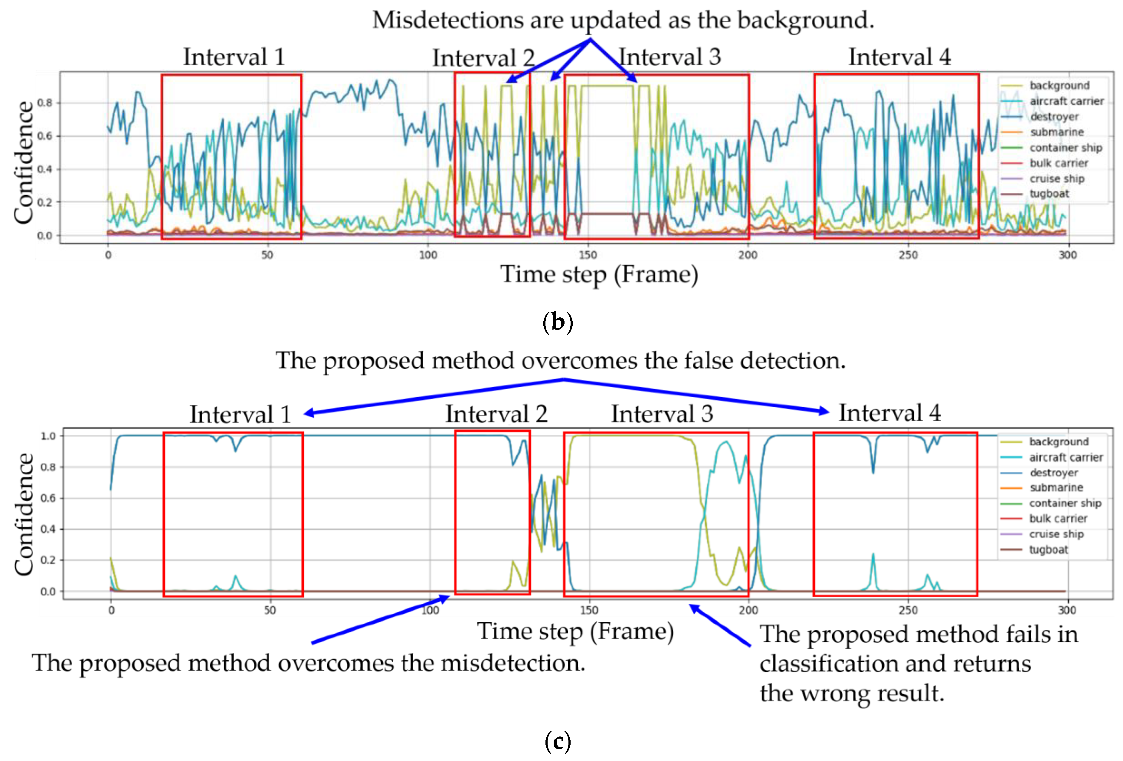
Figure 9.
Captured images from Interval 1.

Figure 10.
Captured images from Interval 2.
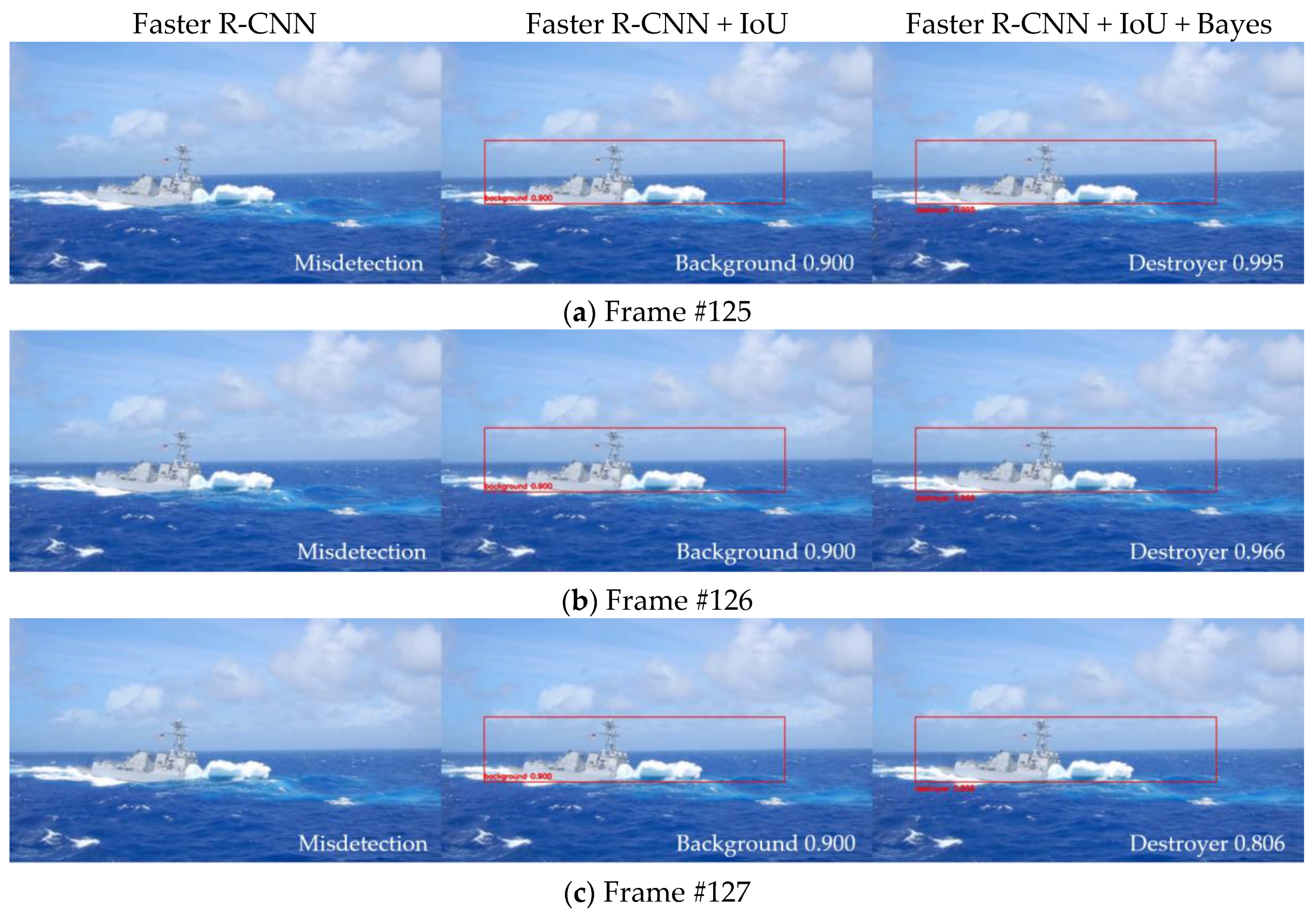
Figure 11.
Captured images from Interval 4.


Table 1.
Classes in the ship dataset.
| 1 | 2 | 3 | 4 | 5 | 6 | 7 | 8 | |
|---|---|---|---|---|---|---|---|---|
| Label | Aircraft carrier | Destroyer | Submarine | Bulk carrier | Container ship | Cruise ship | Tugboat | Back-ground |
Table 2.
The number of images in the ship dataset.
| Class | Training Set | Test Set | Subtotal |
|---|---|---|---|
| Aircraft carrier | 750 | 250 | 1000 |
| Destroyer | 750 | 250 | 1000 |
| Submarine | 750 | 250 | 1000 |
| Container ship | 750 | 250 | 1000 |
| Bulk carrier | 750 | 250 | 1000 |
| Cruise ship | 750 | 250 | 1000 |
| Tugboat | 750 | 250 | 1000 |
| Total | 5250 | 1750 | 7000 |
Table 3.
Results of the single image detection.
| Class | AP (%) |
|---|---|
| Aircraft carrier | 90.56 |
| Destroyer | 87.98 |
| Submarine | 90.22 |
| Container ship | 99.60 |
| Bulk carrier | 99.59 |
| Cruise ship | 99.59 |
| Tugboat | 95.01 |
| mAP | 94.65 |
Table 4.
The change of the class and the confidence of the destroyer.
| Algorithm | Faster R-CNN | Faster R-CNN + IoU | Faster R-CNN + IoU + Bayes | ||||
|---|---|---|---|---|---|---|---|
| Interval | Frame | Class | Confidence | Class | Confidence | Class | Confidence |
| 1 | 19 | Aircraft Carrier | 0.420 | Aircraft Carrier | 0.420 | Destroyer | 0.999 |
| 20 | Aircraft Carrier | 0.403 | Aircraft Carrier | 0.403 | Destroyer | 0.999 | |
| 21 | Aircraft Carrier | 0.539 | Aircraft Carrier | 0.539 | Destroyer | 0.997 | |
| 22 | Destroyer | 0.403 | Destroyer | 0.403 | Destroyer | 0.998 | |
| 23 | Destroyer | 0.433 | Destroyer | 0.433 | Destroyer | 0.999 | |
| 24 | Aircraft Carrier | 0.548 | Aircraft Carrier | 0.548 | Destroyer | 0.997 | |
| 25 | Destroyer | 0.463 | Destroyer | 0.463 | Destroyer | 0.998 | |
| 26 | Destroyer | 0.609 | Destroyer | 0.609 | Destroyer | 0.999 | |
| 27 | Destroyer | 0.611 | Destroyer | 0.611 | Destroyer | 0.999 | |
| 28 | Destroyer | 0.420 | Destroyer | 0.420 | Destroyer | 0.999 | |
| 29 | Aircraft Carrier | 0.434 | Aircraft Carrier | 0.434 | Destroyer | 0.999 | |
| 2 | 118 | Destroyer | 0.546 | Destroyer | 0.546 | Destroyer | 0.999 |
| 119 | Misdetection | 0 | Background | 0.900 | Destroyer | 0.999 | |
| 120 | Destroyer | 0.508 | Destroyer | 0.508 | Destroyer | 0.999 | |
| 121 | Destroyer | 0.454 | Destroyer | 0.454 | Destroyer | 0.999 | |
| 122 | Destroyer | 0.672 | Destroyer | 0.672 | Destroyer | 0.999 | |
| 123 | Destroyer | 0.432 | Destroyer | 0.432 | Destroyer | 0.999 | |
| 124 | Misdetection | 0 | Background | 0.900 | Destroyer | 0.999 | |
| 125 | Misdetection | 0 | Background | 0.900 | Destroyer | 0.995 | |
| 126 | Misdetection | 0 | Background | 0.900 | Destroyer | 0.966 | |
| 127 | Misdetection | 0 | Background | 0.900 | Destroyer | 0.806 | |
| 128 | Destroyer | 0.486 | Destroyer | 0.486 | Destroyer | 0.847 | |
| 4 | 234 | Destroyer | 0.612 | Destroyer | 0.612 | Destroyer | 0.999 |
| 235 | Aircraft Carrier | 0.611 | Aircraft Carrier | 0.611 | Destroyer | 0.999 | |
| 236 | Aircraft Carrier | 0.648 | Aircraft Carrier | 0.648 | Destroyer | 0.999 | |
| 237 | Aircraft Carrier | 0.616 | Aircraft Carrier | 0.616 | Destroyer | 0.990 | |
| 238 | Aircraft Carrier | 0.521 | Aircraft Carrier | 0.521 | Destroyer | 0.983 | |
| 239 | Aircraft Carrier | 0.630 | Aircraft Carrier | 0.630 | Destroyer | 0.955 | |
| 240 | Aircraft Carrier | 0.642 | Aircraft Carrier | 0.642 | Destroyer | 0.758 | |
| 241 | Destroyer | 0.858 | Destroyer | 0.858 | Destroyer | 0.974 | |
| 242 | Destroyer | 0.870 | Destroyer | 0.870 | Destroyer | 0.997 | |
| 243 | Destroyer | 0.814 | Destroyer | 0.814 | Destroyer | 0.999 | |
| 244 | Aircraft Carrier | 0.575 | Aircraft Carrier | 0.575 | Destroyer | 0.998 | |
| 245 | Destroyer | 0.766 | Destroyer | 0.766 | Destroyer | 0.999 | |
| 246 | Destroyer | 0.801 | Destroyer | 0.801 | Destroyer | 0.999 | |
| 247 | Destroyer | 0.689 | Destroyer | 0.689 | Destroyer | 0.999 | |
| 248 | Destroyer | 0.639 | Destroyer | 0.639 | Destroyer | 0.999 | |
| 249 | Aircraft Carrier | 0.601 | Aircraft Carrier | 0.601 | Destroyer | 0.999 | |
| 250 | Destroyer | 0.670 | Destroyer | 0.670 | Destroyer | 0.999 | |
| 251 | Aircraft Carrier | 0.558 | Aircraft Carrier | 0.558 | Destroyer | 0.999 | |
| 252 | Aircraft Carrier | 0.632 | Aircraft Carrier | 0.632 | Destroyer | 0.998 | |
| 253 | Aircraft Carrier | 0.553 | Aircraft Carrier | 0.553 | Destroyer | 0.997 | |
| 254 | Aircraft Carrier | 0.651 | Aircraft Carrier | 0.651 | Destroyer | 0.991 | |
Table 5.
Performance of ship detection on test videos.
| Class | AP (%) | |
|---|---|---|
| Faster R-CNN | Faster R-CNN + IoU + Bayes | |
| Aircraft carrier | 99.33 | 100.00 |
| Destroyer | 68.67 | 77.61 |
| Submarine | 98.00 | 100.00 |
| Container ship | 76.69 | 88.19 |
| Bulk carrier | 88.00 | 94.67 |
| Cruise ship | 96.33 | 96.97 |
| Tugboat | 98.67 | 100.00 |
| mAP (%) | 89.38 | 93.92 |
© 2018 by the authors. Licensee MDPI, Basel, Switzerland. This article is an open access article distributed under the terms and conditions of the Creative Commons Attribution (CC BY) license (http://creativecommons.org/licenses/by/4.0/).
Share and Cite
MDPI and ACS Style
Kim, K.; Hong, S.; Choi, B.; Kim, E. Probabilistic Ship Detection and Classification Using Deep Learning. Appl. Sci. 2018, 8, 936. https://doi.org/10.3390/app8060936
AMA Style
Kim K, Hong S, Choi B, Kim E. Probabilistic Ship Detection and Classification Using Deep Learning. Applied Sciences. 2018; 8(6):936. https://doi.org/10.3390/app8060936
Chicago/Turabian StyleKim, Kwanghyun, Sungjun Hong, Baehoon Choi, and Euntai Kim. 2018. "Probabilistic Ship Detection and Classification Using Deep Learning" Applied Sciences 8, no. 6: 936. https://doi.org/10.3390/app8060936
Note that from the first issue of 2016, this journal uses article numbers instead of page numbers. See further details here.