Effects of Regular Waves on Propulsion Performance of Flexible Flapping Foil

1
College of Engineering, Ocean University of China, Qingdao 266100, China
2
Beijing Aerospace Unmanned Vehicles System Engineering Research Institute, Beijing 100094, China
3
School of Civil Engineering, Qingdao University of Technology, Qingdao 266033, China
4
Cooperative Innovation Center of Engineering Construction and Safety in Shandong Blue Economic Zone, Qingdao 266033, China
5
Science and Technology on Underwater Vehicle Laboratory, Harbin Engineering University, Harbin 150001, China
*
Authors to whom correspondence should be addressed.
Appl. Sci. 2018, 8(6), 934; https://doi.org/10.3390/app8060934
Submission received: 26 April 2018
/
Revised: 28 May 2018
/
Accepted: 1 June 2018
/
Published: 5 June 2018
Abstract
:Featured Application
This work is meaningful for the bionic unmanned underwater vehicle to improve its navigation performance near the sea surface, increase its endurance and reduce its ocean pollution.
Abstract
The objective of the present study is to analyze the effects of waves on the propulsive performance and flow field evolution of flexible flapping foil, and then offer a way to take advantage of wave energy. The effects of regular waves on the propulsive performance of a two-dimensional flexible flapping foil, which imitated the motion and deformation process of a fish caudal fin, were numerically studied. Based on computational fluid dynamic theory, the commercial software Fluent was used to solve the Reynolds-averaged Navier–Stokes equations in the computational domain. Several numerical models were employed in the simulations, which included user-defined function (UDF), numerical wave tank (NWT), dynamic mesh, volume of fluid (VOF), post-processing, and analysis of the wake field. The numerical tank was also deep enough, such that the tank bottom had no influence on the surface wave profile. First, the numerical method was validated by comparing it with experimental results of rigid foil, flapping under waves. The effects of three key wave parameters on the propulsive performance of flexible and rigid foils were then investigated; the results show that higher performance can only be obtained when the motion frequency of the foil was equal to its encounter frequency with the wave. With this precondition, foils were able to generate higher thrust force at larger wave amplitudes or smaller wavelengths. Similarly, the percentage of wave energy recovery by foils was higher at smaller wave amplitudes or wavelengths. From a perspective of wake field evolution, increasing foil velocity (relative to water particles of surrounding waves), could improve its propulsive performance. In addition, flexible deformation of foil was beneficial in not only enhancing vortex intensity but also reducing the dissipation of vortices’ energy in the flow field. Therefore, flexible foils were able obtain a better propulsive performance and higher wave energy recovery ability.
1. Introduction
In recent years, many countries have paid more attention to ocean scientific research and resource exploration [1,2,3]. As a result, ocean delivery platforms with better performance have been the focus of research, in which unmanned underwater vehicles (UUVs) play an important role. The UUV has been widely used in various missions of ocean development [4] owing to its excellent environmental adaptation and scientific-observation abilities. However, a conventional UUV usually uses a screw propeller to provide thrust force, and this design has certain shortcomings; such as the propulsive system occupying a large space, consuming more energy, and a higher noise level. However, a bionic propulsor, which imitates the flapping caudal fin of fish, has several advantages; including higher efficiency, better maneuverability, lower noise, coupling of propulsion and control systems, etc. [5,6]. In addition, fish can utilize the surrounding unstable flow field energy using their caudal fin to improve swimming performance [7,8,9,10]. Therefore, studies on the propulsive performance and flow field evolution mechanism of bionic foil, flapping near the wave surface, are meaningful for the UUV in many aspects; such as utilizing wave favorable impact on foils propulsion, improving UUV navigation performance near the sea surface, increasing its endurance, and reducing ocean pollution.
When operating at sea, a UUV, propelled by a bionic propulsor, needs to navigate near the surface for a long time in various situations (such as data exchange). During this time, wave motions strongly affect the surrounding flow field of the UUV and its hydrodynamic performance. Another key issue is that most UUVs use gas or battery as their power source, which means that they have limited endurance and cause pollution easily. However, a new idea was proposed recently that suggested that UUVs extract energy from surrounding flows as their driving power or auxiliary propulsion [11], as fish do. Similar to this idea, researchers have conducted studies on the application of flapping foils near the wave surface as an auxiliary propulsor for ships [12,13,14], but fewer studies have been done for UUVs.
Researchers have analyzed the hydrodynamic performance of the flapping foil in an infinite flow field, which means the whole flow field is filled with water and there is no free surface. They usually focus on its mechanical parameters and flow field distribution; such as thrust force, resistance, input power, usable power, propulsive efficiency, and instantaneous vortex shape near the foil. Esfahani [15] investigated the effect of caudal length on the hydrodynamic performance of flapping foils. In detail, Esfahani considered that the hydrodynamic performance of a flapping foil is optimum at lower and higher Strouhal numbers (St < 0.2 and St > 0.6). Additionally, Esfahani demonstrated the possibility of improving foil propulsive efficiency at moderate Strouhal numbers (0.2 < St < 0.6) by manipulation of caudal length. However, comparing with rigid foil in above studies, a flexible foil is more similar to the caudal fin of fish. Therefore, Zhu [16] simply treated the flexible foil as an inextensible filament. Then, Zhu used a solver to investigate the hydrodynamic effects of passive flexibility in chord direction on a self-propelled plunging foil in two-dimensions—incompressible and laminar flows. The solver coupled the immersed boundary method for the flow and the finite difference method for the structure. Considering the flexible deformation in a span-wise direction of bionic caudal fin, Zhou [17,18] found that its performance could be improved by adjusting the motion and flexibility parameters. The span-wise flexibility of caudal fin could increase thrust force with high propulsive efficiency. In order to obtain real velocity and vorticity fields of the foil, Lee [19] then employed two-dimensional Digital Particle Image Velocimetry (DPIV), using hydrogen bubbles as seeding particles, to study the flow physics of a hydrofoil in angular reciprocating motion with negligible free-stream velocity to reveal the effects of aspect ratio on its hydrodynamic performance. Their results suggested that a lower aspect-ratio could improve thrust of the foil when it starts from rest, but at the expense of efficiency.
After looking at a steady infinite flow field, researchers have begun to study the mechanism of fish utilizing unsteady flow field energy from the perspective of multi-body disturbance. Shao [20] numerically investigated the hydrodynamic performances of a fishlike undulating foil in the wake of a D-section cylinder by using a modified immersed boundary method. Firstly, Shao observed that the foil without undulation in the vortex street could gain a thrust, as a result of the fact that the passing vortices produce reverse flows with respect to the mainstream in vicinity of the foil surface. An undulating foil is then placed behind the D-section cylinder; Shao found that the undulation of foil plays different roles in its propulsion when the distance between foil and cylinder is changed. In Shao’s studies, the D-section cylinder remains still. Different with Shao’s model, Augier [21] studied a propulsion system which was made up by tandem hydrofoils experimentally and numerically. An experimental measurement system is then developed to extract hydrodynamic loads on the foils and capture their twisting deformation during operation. The measuring data allowed researchers to assess the efficiency of the propulsion system as a function of travel speed and stroke frequency. Based on the Augier study, Liu [22] discussed the distance between foils, pitch angle, and other parameters’ effects on tandem foils’ propulsive performance. By analyzing flow field disturbance between foils, effective ways to improve propulsor performance were proposed. Meanwhile, Xu [23] analyzed the hydrodynamic performance of two flapping foils with the tandem configuration, while the velocity potential theory and the boundary element method were introduced to study the interactions of the vortices and the foils. Xu then found the optimal global phase shifts for the highest thrust and highest efficiency.
Summarizing the above research, studies on the hydrodynamic performance of the bionic flapping foil that propelled the UUV in deep sea, have obtained excellent results. Most studies on the foils were in unsteady flow fields and focused on the steady obstacle effect on the propulsive performance of the foil, or multi-foil effect on improving system maneuverability. In comparison, for the UUV, fewer studies have been carried out on the complex flow effect; such as waves at sea, on the performance of the nearby foils, especially on the flexible foils. Most existing research was mainly on the basis of using the passive moving rigid foils as an auxiliary propulsion for merchant ships. An early concept has been proposed by some researchers that a flapping foil can be used to extract energy from the unsteady flow field, formed by free-surface waves [24,25]. Indeed, in both experiments and theoretical analyses, it was discovered that a foil, submerging right below the free surface, could propel itself forward by using the energy from the incoming waves [24,26,27]. The application of the flapping foils extracting energy from the uniform flows was first proposed by McKinney and DeLaurier [28]. By applying a non-linear 3D panel method, Belibassakis [29] then dealt with the hydrodynamic analysis of the flapping wings, which were located beneath the hull of a ship and operated in random waves. The ship was travelling at a constant forward speed and the free wake analysis was carried out around the flapping wings to obtain detailed characteristics of the unsteady flow. Their results presented significant thrust production, reduction of ship motion responses, and generation of anti-rolling moment for ship stabilization, over a range of motion parameters. Further, Silva [30] numerically studied the possibility of extracting energy from gravity waves for marine propulsion by a two-dimensional oscillating hydrofoil. The investigated results of the simulation explained the increase of propeller efficiency in gravity waves. In addition, Silva suggested that when some key parameters are correctly maintained, the oscillating hydrofoil could take advantage of sea waves to increase its performance. In Silva’s study, the hydrofoil is defined as rigid. Esmaeilifar [31] simulated unsteady, viscous and turbulent fluid flow around a plunging hydrofoil near the water free surface for different submergence depths and oscillation frequencies. The drag of the hydrofoil shows sudden increment in some critical unsteady parameters, such as Strouhal number and frequency. The main reason for this phenomenon is that waves under the above parameters transfer more momentum. In addition, the free surface affects trailing edge vortices from the foil, and causes the drag increment at all frequencies with submergence depth of 0.5c, and at critical frequency with other submergence depths, where c is the chord length of the foil.
As seen from the above research, most of the authors consider a rigid foil, rather than a flexible foil, as the object of study, even though the caudal fin of fish is usually flexible. In this paper, the ability of a flexible bionic flapping foil to take advantage of waves is numerically studied for UUV propulsion. The commercially available computational fluid dynamics (CFD) software Fluent is used with an unstructured grid, based on Reynolds-averaged Navier–Stokes equations. The free surface waves, as well as motion and deformation of the flexible flapping foil were all implemented by customizing the Fluent solver using a user-defined function (UDF) technique. In addition, dynamic mesh technology and post-processing capabilities was fully used. The aim of this study is to investigate the hydrodynamic performance of the flexible foil when it operates near the wave surface, and then analyze ways to reduce the adverse influence of wave movements on the foil performance to utilize wave energy propulsion [27,30,32]. Moreover, vortex forming, fusing, shedding and dissipating processes caused by the foil are discussed. The objectives are to develop a numerical estimation method that can predict the performance of the flexible flapping foil in a wave field.
2. Description and Numerical Model of the Foil under Waves
2.1. Description of the Foil under Waves
In our study, the rigid or flexible foil shows heaving and pitching motions in regular waves. The numerical model is in two dimensions, as shown in Figure 1, in which hl is the submergence depth of the foil’s pitching center, c is the chord length of the foil, and hw is the water depth of the fluid domain. Wave field is set as a regular wave with wavelength λ and wave height H = 2a, where a is wave amplitude. The origin point of the geodetic coordinate system xoy in Figure 1 is located at the interface between the water domain and the air domain, while the positive direction of the x axis is parallel to the wave propagating direction and the y axis point upwards to the air domain from the water domain. In numerical simulations, the foil is fixed in the direction of x axis and its horizontal average advancing velocity is transferred to the uniform water inflow velocity, shown as V0 in Figure 1. Similarly, the origin point of the local coordinate system x1o1y1 for the foil is located at its leading edge point, meanwhile this point is also the pitching center of the foil. L is the horizontal distance between the origins of the xoy and x1o1y1 coordinate systems.
In order to capture the wave surface deformation, the volume of fluid (VOF) method is adopted and then the numerical wave tank (NWT) can be built, in which the regular progressive waveform can be expressed as:
where k is the wave number, k = 2π/λ. ω0 is the encounter frequency and for deep water conditions:
where g is the gravitational acceleration. Imitating the motion of the caudal fin of fish, we simply define the foil movement in harmonic mode coupling in two degrees of freedom—heave and pitch. Based on the above assumption, the foil motion can be described in local coordinates as:
where y1(t) and θ(t) represent the vertical and angular displacement of the foil in local coordinates, while y0 and θ0 represent the heaving amplitude and maximum pitching angle of the foil, respectively. f is the motion frequency of foil and defines the phase difference between heaving and pitching motions of the foil. Meanwhile, ψ is the phase difference between the foil motion and the wave motion, and ψ decides the foil motion attitude when it is meeting a wave crest or trough.
In addition, for the flexible foil, its deformation is defined along the chord direction. According to reference [33], the deforming offset δy of the foil to the initial position versus time can be expressed as:
where δc is the deforming amplitude. f is the deforming frequency and assumed to be equal to the motion frequency of the foil in this paper. x1 is the distance between a location on the foil and its leading edge point, that is, the x1 axis value in the local coordinate system of Figure 1. s and ε are the controlling coefficients for deformation and s, ε >1. According to Equation (5), a larger s makes the flexible deformation closer to the leading edge of the foil, while ε makes it closer to the trailing edge. is the phase difference between the deformation and the heaving motion of the foil. In this paper, we take δc/c = 0.2, s = 100, ε = 2.0, = −90°. Further details about the deformation of flexible foil can be found in [33].
2.2. Function of Hydrodynamic Performance
In numerical simulations based on a CFD model, the thrust force Fx and the lateral force Fy in the direction of the x1 and y1 axes, respectively, as well as the moment M around the pitching center of the foil, can be obtained by integrating the pressure and viscous force of each element along the surface of the foil in different axis directions. Non-dimensional coefficients corresponding to the above parameters can be expressed as:
where Ct, Cl, Cm are the non-dimensional thrust force coefficient, the lateral force coefficient and the moment coefficient, respectively, and ρ is the water density. The instantaneous input power Pi and the output power Po can be expressed as [33]:
As in Equation (6), the input power coefficient Cpi and the output power coefficient Cpo can be defined as:
Based on Equations (3) and (4) and Equations (6) and (7), the propulsive efficiency of the flapping foil η, can be obtained as:
where y1’(t) and θ’(t) are the time derivatives of y1(t) and θ(t) in Equations (3) and (4), that is, the linear and angular velocity of foil, respectively. CT is the average thrust force coefficient, .
In order to analyze the wave energy utilization ability of the foil, the average power of a regular wave experienced by the foil, with unit width Pw and its corresponding coefficient Cpw, can be deduced by the water wave theory:
where cg is the group celerity of the wave (i.e., the transferring velocity of wave energy passing through a certain vertical plane in space and an integrated water volume), and cg equals half the wave celerity cw in deep water, (i.e., cg = cw/2 = (g/k)0.5/2). Based on Equation (10), we can continually define the wave power recovering coefficient Cpr [30], i.e., Cpr = Cpow − Cpon, in which Cpow is the output power coefficient when the foil is with the presence of waves, while Cpon is that when the foil is under calm water surface with the same submergence as in waves. Finally, the percentage of wave energy recovery [30] for a flapping foil ηr can be expressed as ηr = Cpr/Cpw.
2.3. Numerical Method and Model of the Foil under Waves
In these numerical simulations, the flow field is considered viscous and incompressible. Therefore, the continuity and momentum equations are:
where ui and uj are the transient velocity components, while ui′ and ui′ are the fluctuating velocity components. pr is the transient pressure and represents the mean value of . Si is the source item and is the sum of all other force components that do not belong to the transient term, convective term, or diffusive term of the governing equations. μ is the kinematic viscosity coefficient. In addition, the subscripts i, j = 1, 2 in Equations (11) and (12) identify the components along the x and y axis, respectively.
The standard k-ε turbulence model, which has been commonly used, has some deficiencies when applied to the simulation of strongly swirling flow, curved wall flow, and curved streamline flow [34]. The renormalization group (RNG) k-ε two-equation model is applied in this paper. This scheme differs from the standard k-ε turbulence scheme, as it includes an additional sink term in the turbulence dissipation equation to account for non-equilibrium strain rates and employs different values for the model coefficients [35]. Therefore, the RNG k-ε model can deal with the flows with high strain rate and large streamline curvature, such as the flow field of waves and around foils.
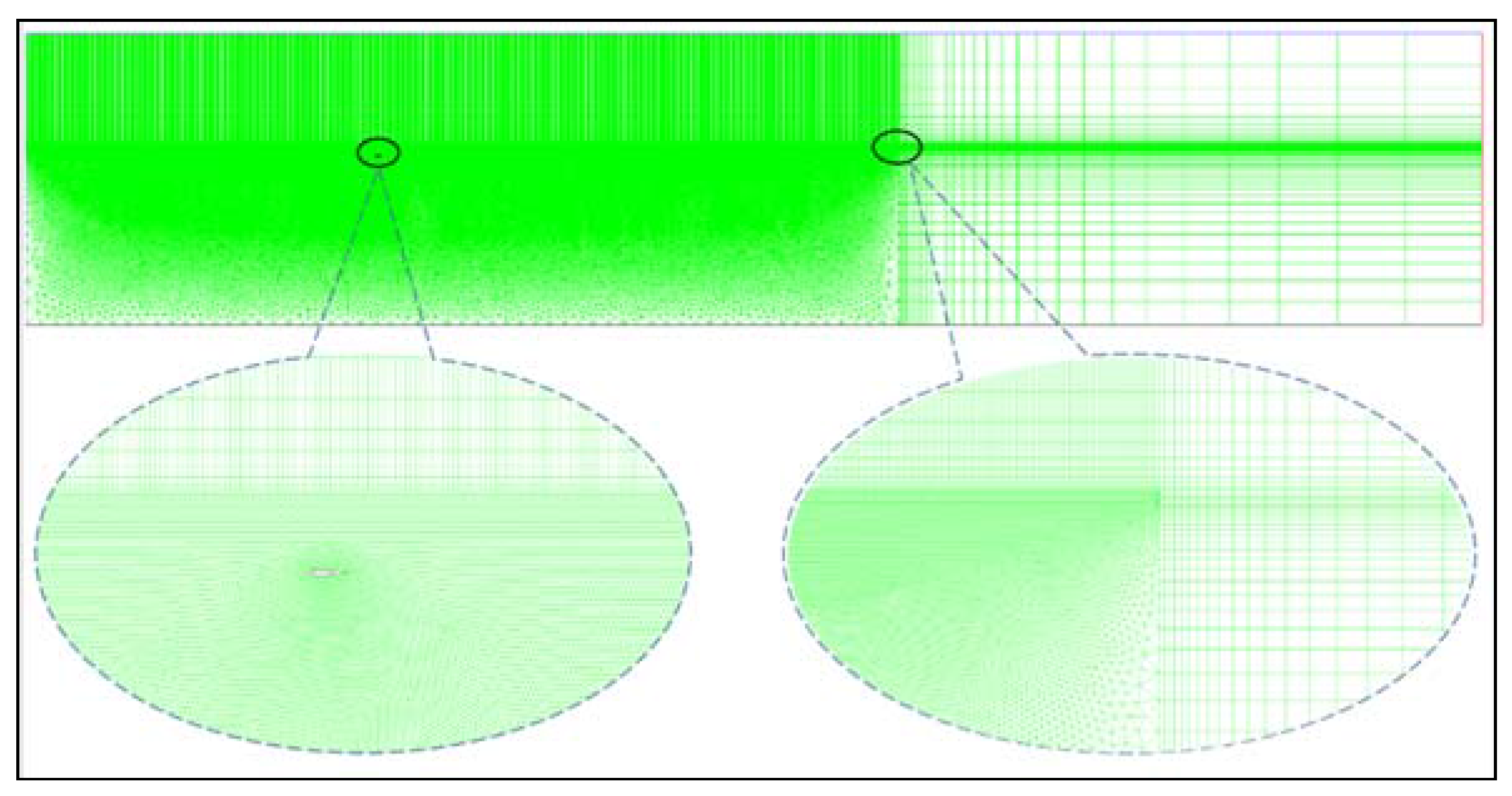
The length of the NWT is L = 5λ. The computational domain is divided in several zones, including air zone, stable waveform zone, and artificial damping zone, as shown in Figure 2. The ratio of the stable waveform zone length to the artificial damping zone length is 3:2 and the foil is placed at 2/5 the stable waveform zone length from the left boundary of the NWT. The boundary conditions of the computational domain is also given in Figure 2. The mesh in the whole computational domain is shown in Figure 3. The stable waveform zone is modelled with an unstructured grid in order to validate the dynamic mesh and re-mesh technologies to ensure good-quality mesh during foil motion. Meanwhile, a structured grid is adopted to model the air domain and the artificial damping domain to improve solving efficiency. The grid near the foil and the free wave surface is densified to satisfy computational accuracy. The meshes of the air zone, stable waveform zone, and artificial damping zone have 12,000, 179,000, and 2000 elements, respectively. The mesh scheme was selected based on reference [30] and a sensitivity analysis was also performed. We selected the fine mesh to obtain a more accurate flow field.
In Figure 3, a regular wave is produced from the water inlet boundary by defining the inflow velocity component. Wave generation equations are implemented in the Fluent solver by programming a UDF. In addition, the height of the air zone is ha = λ/4. The water depth of the NWT is hw = 3λ/4 and it is deep enough that the tank bottom has no influence on the surface wave profile. Therefore, the velocity potential of 2D regular waves in our simulations can be given as:
where ωw is the circular frequency of the wave’s simple harmonic motion, ωw = (gk)0.5. We take the derivative of Equation (13) in the horizontal and vertical directions and obtain the corresponding velocity components of wave generation equations:
As mentioned above, Equation (14) can be programed in the UDF to produce regular waves. In addition, the inflow velocity V0 should be considered in the UDF by adding V0 to the horizontal velocity component of Equation (14). When y > 0, i.e., in the air zone of Figure 3, we define u = V0 and v = 0.
At the end of the numerical zone, an artificial damping zone is applied, and in this domain the wave energy is gradually dissipated in the direction of wave propagation to prevent wave reflection. In order to minimize the possible wave reflection at the entrance of the damping zone and maximize the wave energy dissipation, the length of the damping zone should be equal to one or two times the wavelength. Moreover, the numerical zone needs to transition the damping zone smoothly. A numerical source term ρλdUi is introduced into the momentum equation [36], that is:
where Ui means velocity component and U1 = u, U1 = v. λd is the artificial damping coefficient, which can be defined as follows [37]:
where γ is the controlling coefficient, and it is chosen based on the computational domain and wavelength. Subscript s and e signify the start and end points of the damping zone, respectively. Subscript b and fs signify the bottom and free surface of the NWT, respectively. In the geodetic coordinate system of this paper, x0 = 3λ and x1 = 5λ, then from Equation (16), we can see that this source term works only in the damping zone.
3. Validation of the Numerical Method
3.1. Validation of the Numerical Wave Tank
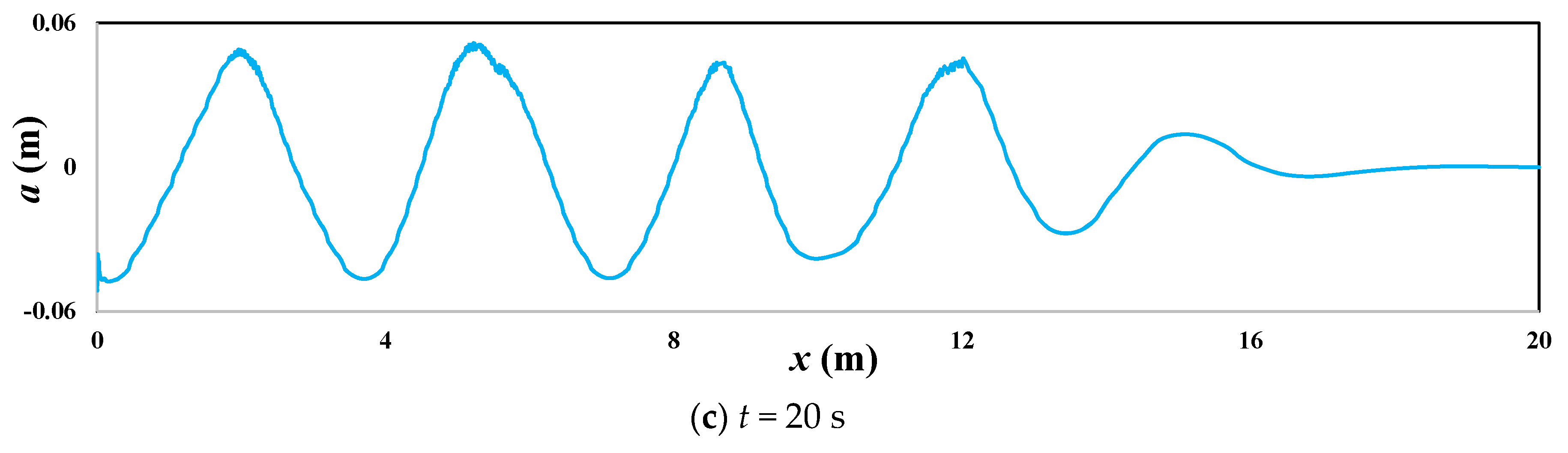
In order to validate the wave generation equations and the artificial damping effect, we first built a numerical wave tank with wavelength λ = 4 m and wave amplitude a = 0.048 m, V0 = 0.28 m/s, in which the foil was not placed. From the numerical model, we then obtained free surface time series at different positions (2 m, 6 m) and compared the wave amplitude versus time with analytic results, and the waveform at t = 20 s of the NWT, as shown in Figure 4, in which “ana. simu” means the analytic simulation process and “num. simu” means the numerical simulation process proposed in this paper.
As shown in Figure 4a,b, the numerical wave amplitudes keep steady and their time series matches the analytic one. In Figure 4c, wave amplitude then drops in the artificial damping zone. Based on Figure 4, the wave generation equations and artificial damping in this paper are valid and the boundaries of the NWT do not affect the waveform at the foil’s position. In addition, the longer the distance between the left boundary of the NWT and the measured position, the longer the time to form a stable waveform and the larger the difference between numerical and analytic waveforms. This phenomenon means wave energy dissipates during its propagation because of the viscous effect of water. This will occur in physical experiments as well. However, the wave amplitudes remains constant at the certain location of the NWT in the time domain.
3.2. Validation of Numerical Simulations
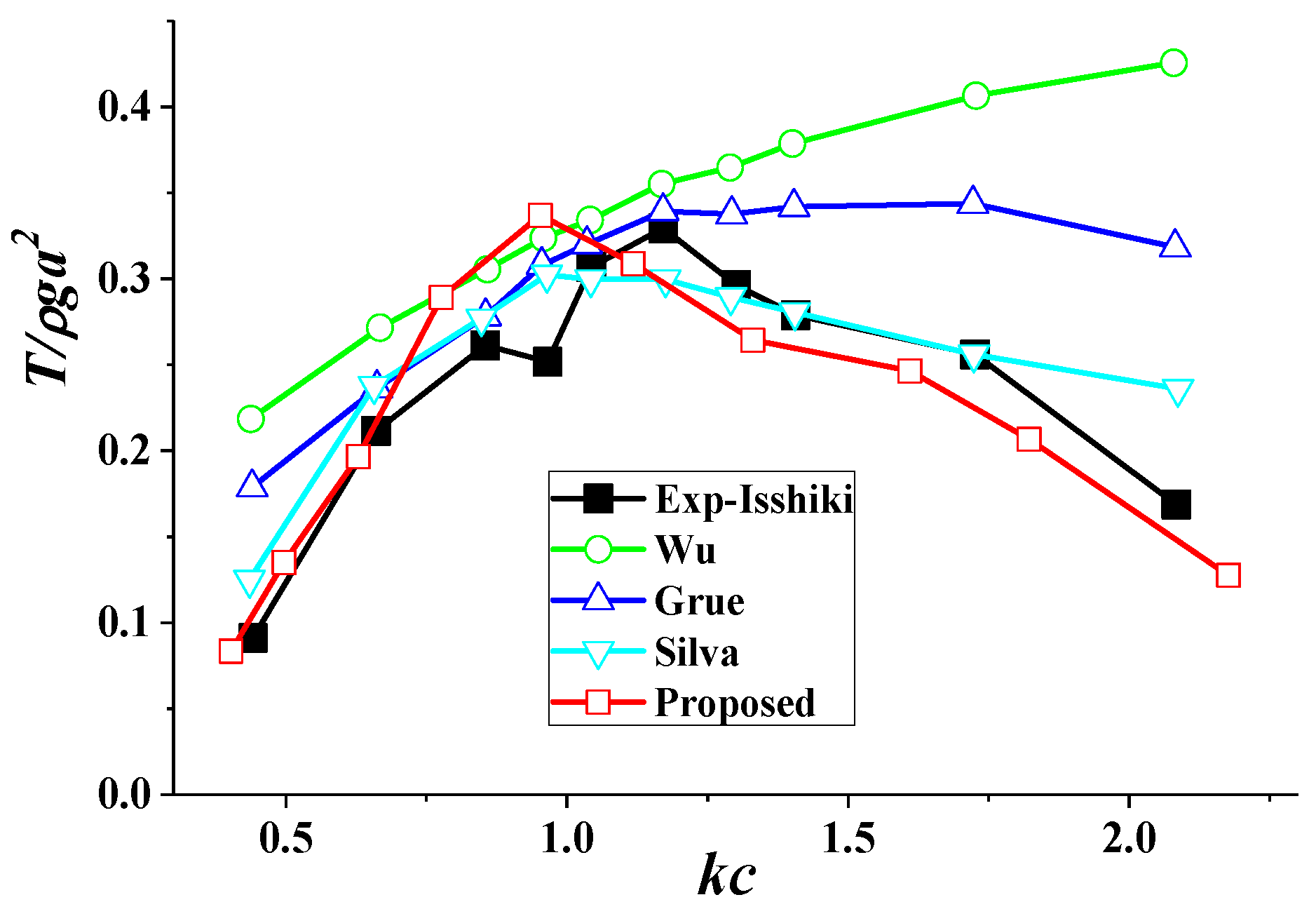
As mentioned previously, a few experimental studies on active flexible flapping foil can be compared, so in this section, we chose an experiment of the rigid foil with a passive motion under waves, carried out by Isshiki [26] in 1984, to validate the numerical simulations. Isshiki’s experiment was carried out in a tank 25 m × 1 m × 0.71 m (length × breath × depth) and the foil had a profile of NACA0015 and 0.4 m chord length. The foil was attached to a carriage by springs and the carriage moved horizontally with constant velocity. It is known that any object’s motions have a one-to-one correspondence with its mechanical performance. Therefore, although the foil in this experiment was moving passively, we could still use the active moving foil in numerical simulations on the condition that they all followed the same motion law. The passive and active foil can then obtain the same thrust force. In our simulations, V0 is equal to the constant velocity of the carriage in the experiments, and the distance between the pitching center and the leading edge point of the foil is 0.12 m, as set in Isshiki’s experiment. In addition, the motion frequency of the foil is set equal to its encounter frequency, while a = 0.048 m.
The numerical results by our method and experimental results from the reference [26] are compared in Figure 5, in which the vertical coordinate represents non-dimensional thrust force and the horizontal coordinate is the product of the wave number and chord length of the foil. For comparison, other numerical results based on the linear theory by Wu [24], the nonlinear theory by Grue et al. [27], and the viscous flow theory by Silva [30] are also given in Figure 5.
From Figure 5, we see that the non-dimensional thrust force first increases and then decreases in the experiments. Comparing four numerical results, we note that all of are in good agreement with Isshiki’s experimental results at larger wavelengths (smaller kc), but when wavelengths are smaller (larger kc), only the results by the method proposed in this paper and Silva’s method are in good agreement with it. Therefore, considering the general trend, the numerical method proposed in this paper seems better and will be used in the next sections.
4. Numerical Results and Analysis
In this paper, the effect of regular waves on the propulsive performance of a flexible foil is investigated, considering the encounter frequency ω0, wavelength λ, and wave amplitude a. Other conditions, such as phase difference, foil motion, and flexible parameters, have been discussed in previous studies. One can find details in references [38,39]. For convenience, we change ω0, λ, and a to ω0/2πf, λ/c, a/c by non-dimensional treatment.
In our analysis, a basic parameter case is given and a controlling variate method is adopted, that is, only one variable of the basic case is changed in every working condition and the others remain constant. Therefore, we give the basic case setting as the inflow constant velocity V0 = 0.1 m/s. The regular wave height is H = 2a = 0.04 m and the wavelength λ = 6.64 m. The foil is profile NACA0012 with the chord length c = 0.1 m and the submergence depth hl = 0.12 m, and the phase difference between the heaving and pitching motion of the foil is = 90°. The foil motion period is T = 2 s = 1/f = 2π/ωf, where ωf is the angular frequency of foil motion. The phase between wave and foil motions is ψ = −90°. For foil flexible deforming, δc = 0.2 c, = −90°, while the controlling coefficients s = 100, ε = 2.0. The heaving amplitude of the foil is y0 = 0.5 c and the pitching angle is θ0 = 15°. The wave encounter frequency ω0 = ωf. In addition, for comparison, the performance in infinite flow field and under calm water of flexible, as well as the rigid foil, have also been calculated, where “infinite” means that no free surface exists and the whole computational domain is filled with water.
Before discussing the results, another important parameter should be mentioned—the submergence depth of foil hl—as the flow under waves in deep water is strongly affected by it. In our preliminary studies based on the above basic case for the flexible foil, with hl changing from 0.12 m to 0.20 m, the average thrust force coefficient CT descends from 3.21 to 2.8 and its decreasing rate slows down. Thus, combined with the following analysis, we can infer that the favorable effect of wave on the foil’s propulsive performance will be reduced with increasing hl and this effect will disappear when hl is deeper than half the wavelength.
4.1. Effect of Wave Encounter Frequency on Foil Performance
In Wu’s [24] opinion, when ω0 = ωf, higher utilization efficiency can be obtained. In this section, this viewpoint will be validated and the effect of ω0/ωf on the flexible foil propulsive performance will be analyzed in detail. In these simulations, different ω0/ωf can be obtained by changing the wavelengths and keeping ωf constant.
With different ω0/ωf, the average thrust force coefficient CT and the utilization wave power coefficient Cpr of the rigid and flexible foil, respectively, are shown in Figure 6, in which “-wave” and “-calm water” represent corresponding parameters of the foil under the waves and the calm water, respectively; in later figures, their meanings are the same.
It is obvious that the peak values of CT and Cpr appear at ω0/ωf = 1; that is, the rigid and flexible foil can obtain higher thrust force and recovered wave power [30] when the foil motion frequency is equal to its wave encountering frequency, as proposed by Wu. Meanwhile, as shown in Figure 6, the thrust force of the foil, whether rigid or flexible, generated under waves, is always larger than that under calm water at any ω0/ωf. Therefore, we can conclude that the wave motions are beneficial to the thrust force generation, no matter what wave frequency the foil encounters. Compared with that under calm water, the thrust force of rigid and flexible foil in waves can be improved 64% and 76%, respectively, at ω0/ωf = 1. In addition, the thrust force and the wave power utilization coefficients of the flexible foil are 13% and 25% larger than those of rigid foil at ω0/ωf = 1 under waves. This phenomenon shows that flexible deformation can improve the propulsive performance of the foil, and this conclusion is in agreement with Zhou [17,18].
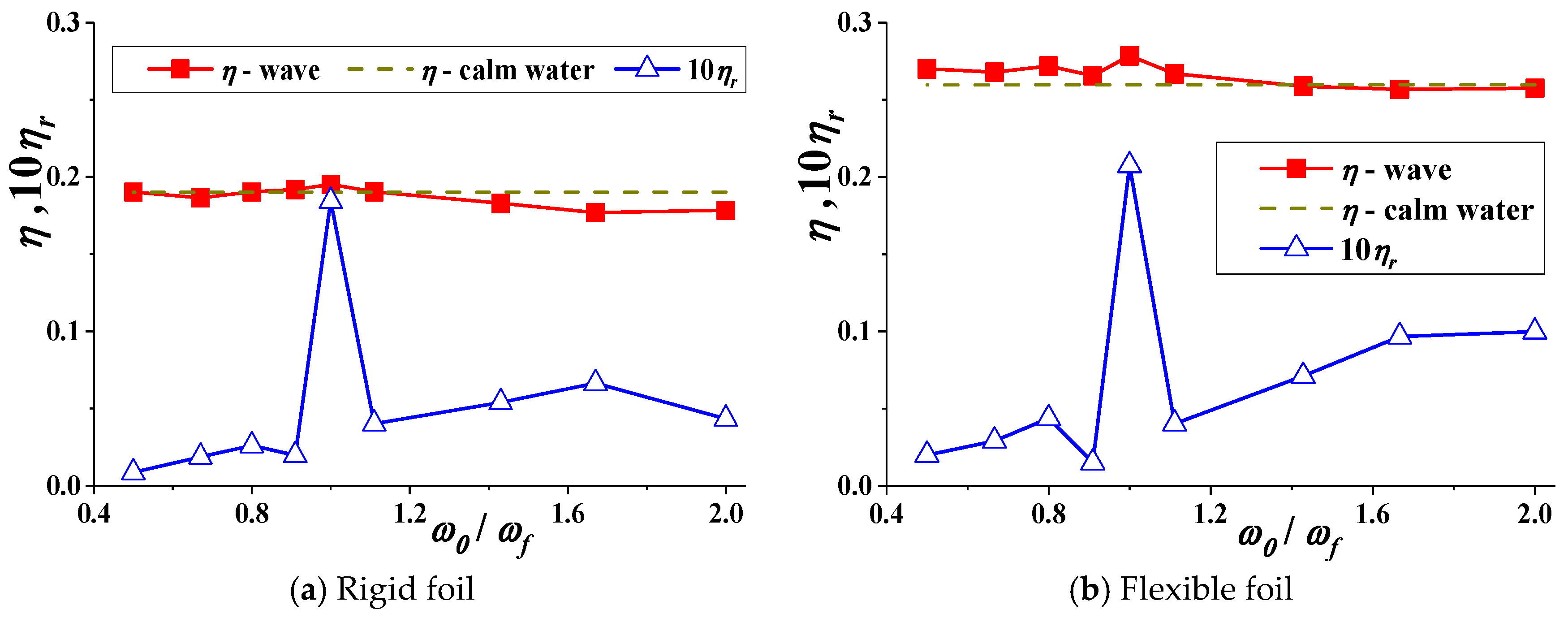
After obtaining CT and Cpr, the propulsive efficiency η and the percentage of wave energy recovery ηr can be calculated; their trends with ω0/ωf are shown in Figure 7.
As seen in Figure 7, when ω0/ωf < 1, the percentage of wave energy recovery ηr of the rigid and flexible foil ascends slightly with increasing ω0/ωf, and reaches peak value rapidly when ω0/ωf is close to 1, where these curve trends validate Wu’s opinion. Obviously, the propulsive efficiency η of the flexible foil is higher than that of rigid foil in various flow field environments, while also reaching η peak value at ω0/ωf = 1 in waves. This value of the flexible foil is 43% higher than that of the rigid foil. Compared with the trends of CT in Figure 6, η changes more smoothly near ω0/ωf = 1. In addition, the propulsive efficiency of the flexible foil and the rigid foil in waves will become smaller than that under calm water when ω0/ωf = 1.2 and 1.5, respectively. Above all, if the motion frequency of foil does not match its encounter frequency, the foil’s propulsive efficiency will be affected adversely, but the flexible deformation can reduce this adverse effect.
4.2. Effect of Wave Amplitudes on Foil Performance
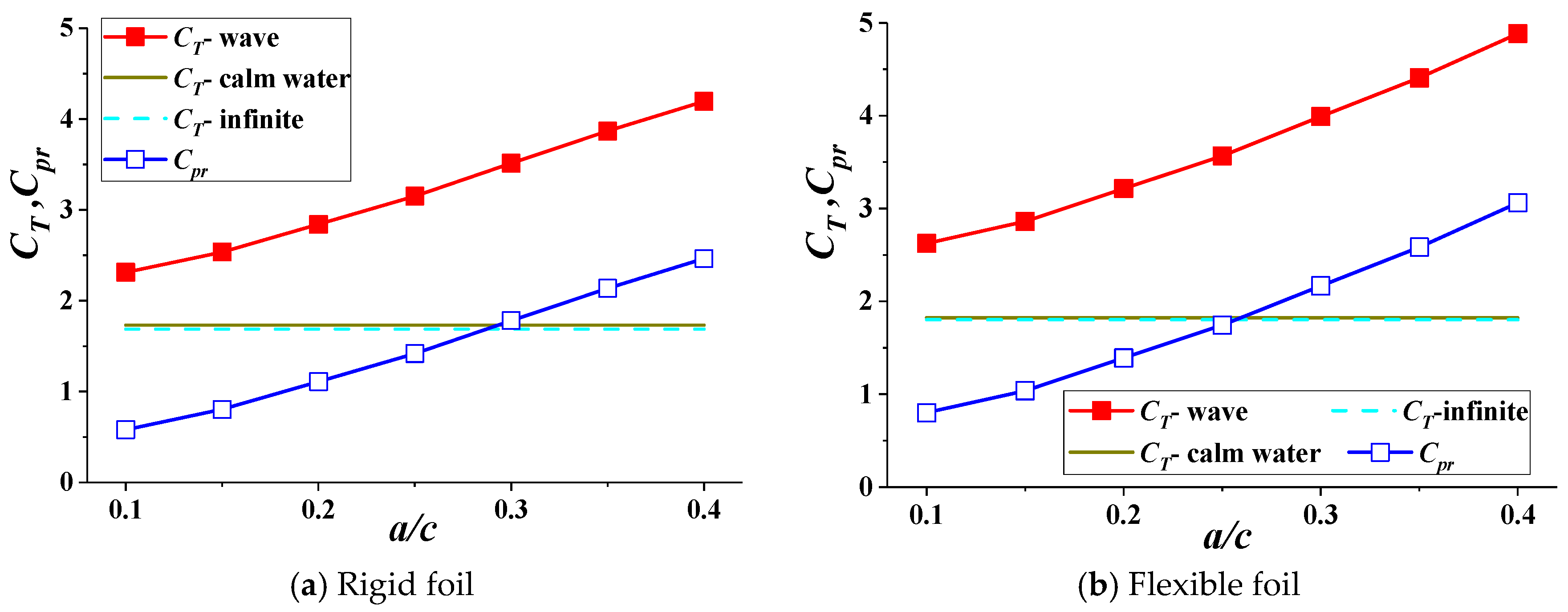
According to Equation (14), a given wave amplitude a denotes a certain velocity of water particles in waves. This motion disturbs the flow field of the nearby foil, thus impacting its hydrodynamic performance. The thrust force coefficient CT and the wave power utilization coefficient Cpr of the foil are shown in Figure 8, relative to the non-dimensional wave amplitude a/c, where “-infinite” means the foil is located in the infinite flow field, and “-calm water” means the foil is located under the calm water surface with the same submergence as in waves. As no wave motion exists in the “infinite” and “calm water” flow fields, corresponding CT and Cpr are constant.
As seen in Figure 8, CT and Cpr ascend with the increasing wave amplitude a/c, and the thrust force of the foil in waves is clearly larger than that in infinite flow fields and under calm water. Compared to calm water, the thrust force of the flexible and rigid foils in waves can be increased by 33.5% and 44.0% at a/c = 0.1, respectively, and by 142.3% and 168.0% at a/c = 0.4, respectively. Meanwhile the force of flexible foil is 13.5% and 16.4% higher than that of rigid foil at a/c = 0.1 and 0.4, respectively. Therefore, the wave motions and the flexible deformation are beneficial in obtaining a higher thrust force. The trend of CT curves in Figure 8 is similar to that of the heaving amplitude of the foil in reference [38]. This phenomenon can be explained as maintaining a constant motion period, and increasing wave amplitudes will increase the velocity of water particles near the foil. Therefore, larger wave amplitudes or foil heaving amplitude can increase the moving velocity of the foil related to its surrounding water particles, and the thrust force can be improved correspondingly. In addition, flexible deformation can also cause this phenomenon, and thus result in higher thrust force than that of rigid foil.
The wave energy utilization power coefficient Cpr of the flexible foil is also higher than that of the rigid foil, but its increment gets smaller with increasing wave amplitudes, specifically, 38.0% and 24.2% higher than the rigid foil at a/c = 0.1 and 0.4, respectively. This means the contribution of the flexible deformation to improving Cpr reduces with decreasing wave amplitudes. After obtaining the thrust force and the wave power utilization coefficients, the propulsive efficiency and the percentage of wave energy recovery can be calculated, as shown in Figure 9.
Changes in wave amplitudes have less influence on foil propulsive efficiency η, as shown in Figure 9. From Figure 8 and Equation (9), in waves, increasing a/c not only increases the thrust force coefficient, but also the lateral force and moment coefficients, which means the input and output power of the foil ascend and then change less in η. However, these values in waves are still larger than under calm water. Although the propulsive efficiency of the foil under a free surface is smaller than that in an infinite flow field, the flexible deformation can reduce this decreasing trend, and the flexible foil η in waves is higher than the rigid foil η in the infinite flow fields. However, increasing wave amplitudes reduces the percentage of wave energy recovery ηr. To summarize, a higher sea state is beneficial to improving the thrust force of the foil, but not wave energy utilization ability. The flexible deformation can produce a larger thrust force, and have fewer adverse effects of the free surface on reducing the propulsive efficiency of the foil.
4.3. Effect of Wavelengths on the Foil Performance
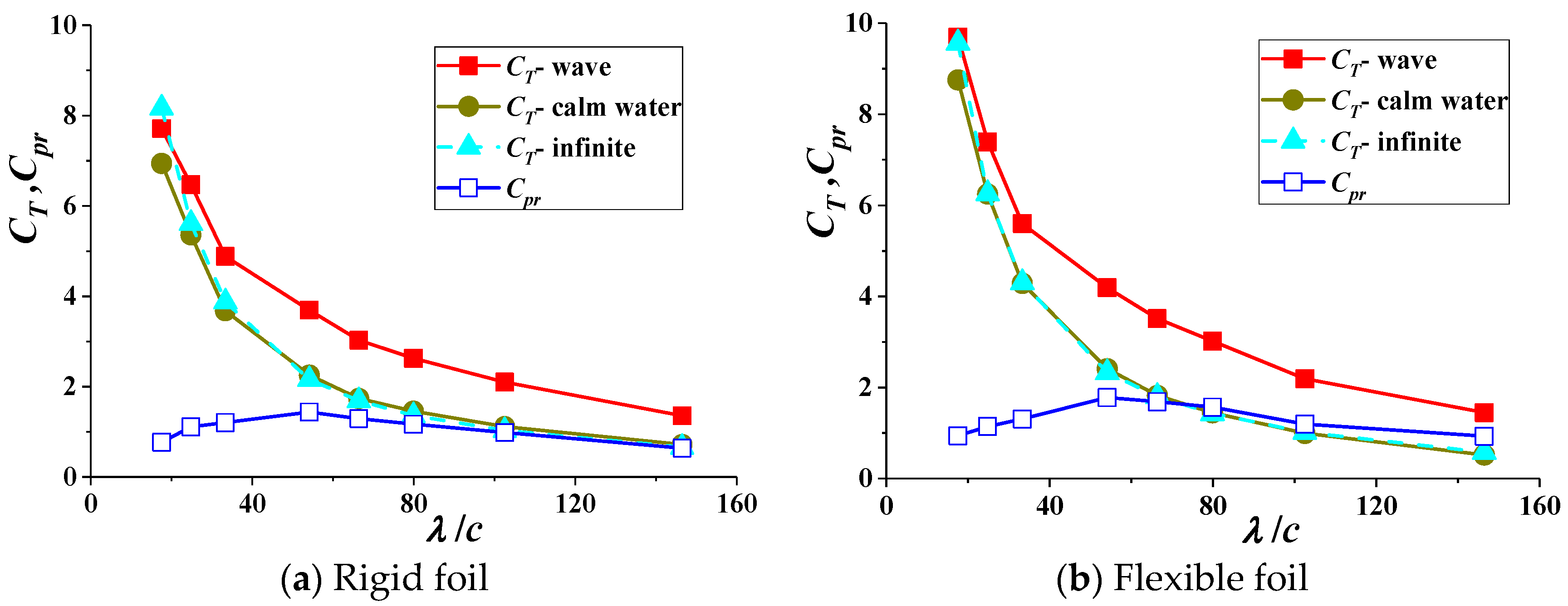
In this section, the effects of wavelengths on the propulsive performance are discussed. Assuming the motion frequency of the foil is equal to its encounter frequency with waves, it should be illustrated that different wavelengths mean different motion periods for the foil in infinite flow fields and under calm water. The thrust force coefficient CT and the wave power utilization coefficient Cpr with the non-dimensional wavelength λ/c can then be calculated, as shown in Figure 10.
The thrust force descends rapidly with increasing wavelength λ/c, because longer wavelengths mean longer motion periods for the foil, so the velocity of the foil, relative to the water particles, will descend in this situation with a given heaving amplitude. As a result, the thrust force of the foil will become smaller. However, as wave motion benefits the thrust force generation, the descending rate of the foil’s thrust force in waves is slower than in infinite flow fields and under calm water. Meanwhile, the wave power utilization coefficient Cpr of the rigid and flexible foils first ascends and then descends with increasing wavelength λ/c. According to its expression, Cpr reflects the difference in the thrust force of the foil between waves and calm water. Therefore, as seen in Figure 10, with larger or smaller wavelengths, the wave effect on improving foil thrust force is limited. In addition, when λ/c ≈ 54, Cpr of the flexible and rigid foil can reach peak values of 1.78 and 1.44, respectively.
The propulsive efficiency η ascends with increasing wavelengths, as shown in Figure 11. For the rigid foil, η in the infinite flow fields is always larger than under the free surface, and the difference gets larger with increasing wavelengths. However, for the flexible foil, the difference of η between the foil in waves and in infinite flow fields is not significant, and the former will be larger than the latter when λ/c > 130. At an arbitrary wavelength, η of the flexible foil is always larger than that of the rigid foil, and is larger by 48.2% and 39.7% when λ/c = 20 and 140, respectively. Differing from the trend of η monotonically increasing with the rigid foil, η of the flexible foil can reach a peak value when λ/c = 100. Combined with Figure 10, it can then be seen that the flexible deformation contributes to a higher thrust force and propulsive efficiency in waves than in infinite flow fields or under calm water.
Similarly, the percentage of wave energy recovery ηr of the rigid foil descends with increasing λ/c, but for the flexible foil, the trend is to first ascend and then descend, and its maximum value appears at λ/c = 60. Meanwhile, ηr of the rigid foil is slightly larger than that of the flexible foil at smaller wavelengths, by 16.5% at λ/c = 20. However, when λ/c = 35, they are approximately equal. Nevertheless, when λ/c > 35, ηr of the flexible foil will be larger than that of the rigid foil, by 31.4% at λ/c = 140. Therefore, we can conclude that the effect of the flexible deformation on improving the percentage of wave energy recovery works with certain wavelengths.
4.4. Effect of Waves on the Foil Wake Field
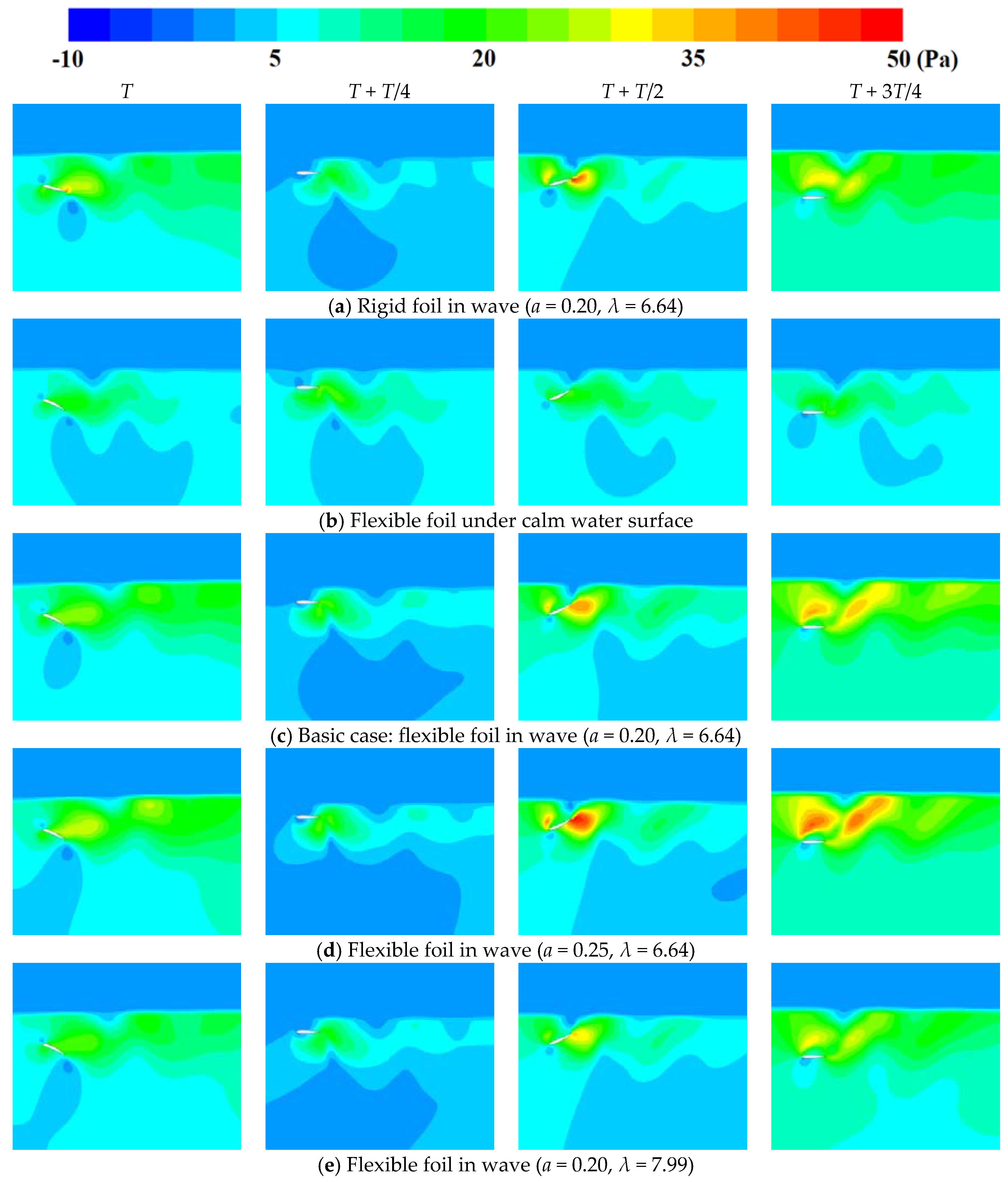
As mentioned above, the wave effect on the foil propulsive performance can be due to water particle motions disturbing the flow field of the foils. As seen in Figure 12, instantaneous dynamic pressure near the foil is given at different times in various conditions. Although the dynamic pressure changes with time and we can obtain this distribution at any time from the Fluent software, several snapshots of the pressure field of characteristic time are selected to analyze the evolution process of flow field near the foil. Based on the Bernoulli equation in hydromechanics, the dynamic pressure can also reflect the water particle velocity and vortex structures. Other parameters, such as turbulent kinetic energy, can also then be obtained by operating on the water particle velocity or post-processing the flow field profile. In addition, Figure 12c shows the flexible foil wake field of the basic case that is described in Section 4.
Comparing Figure 12c,d, there is little difference in vortex intensity between the rigid foil and the flexible foil in waves, so the instantaneous thrust force is approximately equal. But the vortex distribution range of the flexible foil is more concentrated and has better continuity. In addition, the time of vortices shedding from the flexible foil is later than that of the rigid foil. Therefore, the flexible deformation can slow down the shedding of vortices and then reduce energy wasting in a flow field. As a result, the flexible foil can obtain a higher propulsive efficiency.
On comparing Figure 12c,e, different effects of calm water and waves on the flexible foil wake fields are shown. It is obvious that the vortices from the foil in waves are stronger than those under calm water, especially at time T + T/2. From a kinematics perspective, wave motion can increase foil velocity in surrounding water particles and the velocity gradient of the flow field near the foil, thus causing greater vortex intensity. From the perspective of energetics, as the foil utilizes extra wave energy, its wake field can contain more kinetic energy and slow down its vortex merging rate. Meanwhile, the output power of the foil can also be increased and the foil can generate a corresponding larger thrust force. In addition, extra input energy from waves can make the foil obtain a higher propulsive efficiency.
Comparing Figure 12c,d the wave amplitude effect on the wake field of the flexible foil can be seen. The vortex intensity of the foil increases rapidly with larger wave amplitudes, especially at time T + T/2 and T + 3T/4 when the orbital velocity of the foil reverses. The instantaneous maximum thrust force of the foil is then much higher and its average value is increased correspondingly. However, larger wave amplitudes make the foil wake range wider, so more energy is dissipated in the wake field. This makes the foil to not have much higher propulsive efficiency.
Comparing Figure 12c,e, the effect of wavelength on the wake field of the flexible foil can be analyzed. As the foil velocity related to water particles with longer wavelengths is lower than that with shorter wavelengths, the foil’s vortex intensity is also not higher with longer wavelengths, and the foil can only obtain a smaller thrust force. However, the vortex distribution range and the velocity gradient of the foil wake field with longer wavelengths can be smaller than those with shorter wavelengths, which means that only a small amount of energy will dissipate in the flow field and the flexible foil can achieve a relatively higher propulsive efficiency.
5. Conclusions
In this paper, a flexible foil was set to perform coupled heaving and pitching motions under a wave surface. Based on computational fluid dynamics, the propulsive performance of the foil, as well as the wave effect on the foil’s flow field evolution, are investigated by a numerical method. In these simulations, several techniques were employed; which include dynamic mesh, volume of fluid, and wake field analysis.
By changing the wavelength and keeping motion frequency constant, foil could have different encounter frequency relative to waves. We then found that foils could obtain higher propulsive performance and wave energy utilization ability only when their motion frequency was equal to encounter frequency. If this frequency equal condition is not satisfied, the foils’ performance will drop rapidly. Moreover, larger wave amplitudes are beneficial in improving the thrust force of flexible foil up to 142.3% than under calm water surface, but not in obtaining higher utilization efficiency of wave energy and it was less than 5% in our simulations. However, the propulsive efficiency of the flexible foil is less affected by wave amplitudes, and it maintains at about 27%. Smaller wavelengths are beneficial to the flexible foil obtaining a larger thrust force and higher percentage of wave energy recovery. Compared with the largest wavelength in our simulations, these two parameters can be improved up to five and four times, respectively, at the smallest wavelength. Meanwhile, the foil’s propulsive efficiency is higher at larger wavelengths and can be even higher than that in infinite flow filed. After analyzing wake fields of the foil, we found that the wave motion could change the relative velocity of flexible foil to its surrounding water particles in the flow field. This is also the main reason why the foil’s performance is affected by waves. In addition, the flexible deformation of the foil can increase the velocity gradient of its wake field and vortex intensity, and slow down the vortex shedding process from the foil’s trailing edge. As a result, flexible foil can obtain a larger thrust force, higher propulsive efficiency, and wave energy utilization ability in a regular wave environment. In summary, to improve the navigation performance of UUV, propulsion by flexible flapping foils rather than rigid ones is recommended. As the extra input power is extracted from surrounding waves, the foils can obtain better propulsive performance in high sea state without considering their wave energy utilization efficiency.
Author Contributions
P.L. performed the numerical simulations and wrote the paper; Y.L. and S.H. analyzed the data; J.Z. explored the literatures; Y.S. proposed the original idea.
Acknowledgments
The authors wish to acknowledge financial support from the National Natural Science Foundation of China (Grant Nos. 51609220, 51709246), the Fundamental Research Funds for the Central Universities, and Qingdao Postdoctoral Application Research Foundation.
Conflicts of Interest
The authors declare no conflict of interest.
Nomenclature
| UUV | unmanned underwater vehicle | a | wave amplitude |
| DPIV | Digital Particle Image Velocimetry | c | chord length |
| VOF | volume of fluid | λ | wavelength |
| NWT | numerical wave tank | St | Strouhal number |
| CFD | computational fluid dynamics | xoy | geodetic coordinate system |
| RNG | renormalization group | x1o1y1 | local coordinate system |
| hl | submergence depth | V0 | inflow velocity |
| hw | water depth | k | wave number |
| H | wave height | y0 | heave amplitude |
| g | gravitational acceleration | θ0 | maximum pitching angle |
| phase difference between deformation and the heaving motion | phase difference between heaving and pitching motions | ||
| θ(t) | angular displacement | δy | deforming offset |
| ψ | phase difference between foil motion and wave motion | δc | deforming amplitude |
| f | motion frequency | M | moment |
| s, ε | controlling coefficients for deformation | Fy | lateral force |
| y1(t) | vertical displacement | Cl | lateral force coefficient |
| Fx | thrust force | ρ | water density |
| Ct | thrust force coefficient | Po | output power |
| Cm | moment coefficient | Cpo | output power coefficient |
| Pi | input power | CT | average thrust force coefficient |
| Cpi | input power coefficient | Cpw | average power coefficient |
| η | propulsive efficiency | cw | wave celerity |
| cg | group celerity | ηr | percentage of wave energy recovery |
| Pw | average power of a regular wave with unit width | Cpon | output power coefficient under calm water surface |
| Cpr | wave power recovering coefficient | ui′, ui′ | fluctuating velocity components |
| Cpow | output power coefficient with the presence of waves | mean velocity components | |
| ui, uj | transient velocity components | Si | source item |
| mean value of | ha | height of the air zone | |
| pr | transient pressure | ωw | circular frequency of the wave motion |
| μ | kinematic viscosity coefficient | γ | controlling coefficient for damping |
| λd | artificial damping coefficient | T | motion period of foil |
| ωf | angular frequency of foil motion | Ui | velocity component |
References
- Mengerink, K.J.; Van Dover, C.L.; Ardron, J.; Baker, M.; Escobar-Briones, E.; Gjerde, K.; Koslow, J.A.; Ramirez-Llodra, E.; Lara-Lopez, A.; Squires, D.; et al. A Call for Deep-Ocean Stewardship. Science 2014, 344, 696–698. [Google Scholar] [CrossRef] [PubMed]
- Liu, F.S.; Chen, J.F.; Qin, H.D. Frequency response estimation of floating structures by representation of retardation functions with complex exponentials. Mar. Struct. 2017, 54, 144–166. [Google Scholar] [CrossRef]
- Liu, F.; Lu, H.; Ji, C. A general frequency-domain dynamic analysis algorithm for offshore structures with asymmetric matrices. Ocean Eng. 2016, 125, 272–284. [Google Scholar] [CrossRef]
- Rzhanov, Y.; Eren, F.; Thein, M.W.; Pe’Eri, S. An image processing approach for determining the relative pose of unmanned underwater vehicles. In Proceedings of the Oceans 2014, Taipei, Taiwan, 7–10 April 2014; pp. 1–4. [Google Scholar]
- Yu, J.; Tan, M.; Wang, S.; Chen, E. Development of a biomimetic robotic fish and its control algorithm. IEEE Trans. Syst. Man Cybern. Part B 2004, 34, 1798–1810. [Google Scholar] [CrossRef]
- Fish, F.E. Advantages of Natural Propulsive Systems. Mar. Technol. Soc. J. 2013, 47, 37–44. [Google Scholar] [CrossRef]
- Liao, J.C.; Beal, D.N.; Lauder, G.V.; Triantafyllou, M.S. Fish Exploiting Vortices Decrease Muscle Activity. Science 2003, 302, 1566–1569. [Google Scholar] [CrossRef] [PubMed]
- Maertens, A.P.; Triantafyllou, M.S.; Yue, D.K. Efficiency of fish propulsion. Bioinspir. Biomim. 2015, 10, 046013. [Google Scholar] [CrossRef] [PubMed] [Green Version]
- Zhu, Q.; Wolfgang, M.J.; Yue, D.K.P.; Triantafyllou, M.S. Three-dimensional flow structures and vorticity control in fish-like swimming. J. Fluid Mech. 2002, 468, 1–28. [Google Scholar] [CrossRef] [Green Version]
- Liu, F.; Li, H.; Wang, W.; Liang, B. Initial-condition consideration by transferring and loading reconstruction for the dynamic analysis of linear structures in the frequency domain. J. Sound Vib. 2015, 336, 164–178. [Google Scholar] [CrossRef]
- Townsend, N.C.; Shenoi, R.A. Feasibility study of a new energy scavenging system for an autonomous underwater vehicle. Auton. Robots 2016, 40, 973–985. [Google Scholar] [CrossRef]
- Bøckmann, E.; Steen, S. Experiments with actively pitch-controlled and spring-loaded oscillating foils. Appl. Ocean Res. 2014, 48, 227–235. [Google Scholar] [CrossRef]
- Filippas, E.S.; Belibassakis, K.A. Hydrodynamic analysis of flapping-foil thrusters operating beneath the free surface and in waves. Eng. Anal. Bound. Elem. 2014, 41, 47–59. [Google Scholar] [CrossRef]
- Huang, S.W.; Wu, T.L.; Hsu, Y.T.; Guo, J.H.; Tsai, J.F.; Chiu, F.C. Effective energy-saving device of Eco-Ship by using wave propulsion. In Proceedings of the Techno-Ocean, Kobe, Japan, 6–8 October 2016; pp. 566–570. [Google Scholar]
- Esfahani, J.A.; Barati, E.; Karbasian, H.R. Effect of caudal on hydrodynamic performance of flapping foil in fish-like swimming. Appl. Ocean Res. 2013, 42, 32–42. [Google Scholar] [CrossRef]
- Zhu, X.J.; He, G.W.; Zhang, X. Numerical study on hydrodynamic effect of flexibility in a self-propelled plunging foil. Comput. Fluids 2014, 97, 1–20. [Google Scholar] [CrossRef]
- Zhou, K.; Liu, J.; Chen, W. Study on the Hydrodynamic Performance of Typical Underwater Bionic Foils with Spanwise Flexibility. Appl. Sci. 2017, 7, 1120. [Google Scholar] [CrossRef]
- Zhou, K.; Liu, J.; Chen, W. Numerical Study on Hydrodynamic Performance of Bionic Caudal Fin. Appl. Sci. 2016, 6, 15. [Google Scholar] [CrossRef]
- Lee, J.; Park, Y.J.; Cho, K.J.; Kim, D.; Kim, H.Y. Hydrodynamic advantages of a low aspect-ratio flapping foil. J. Fluid Struct. 2017, 71, 70–77. [Google Scholar] [CrossRef]
- Shao, X.M.; Pan, D.Y.; Deng, J.; Yu, Z.S. Hydrodynamic performance of a fishlike undulating foil in the wake of a cylinder. Phys. Fluids 2010, 22, 111903. [Google Scholar]
- Augier, B.; Yan, J.; Korobenko, A.; Czarnowski, J.; Ketterman, G.; Bazilevs, Y. Experimental and numerical FSI study of compliant hydrofoils. Comput. Mech. 2015, 55, 1079–1090. [Google Scholar] [CrossRef] [Green Version]
- Liu, P.; Su, Y.M.; Liao, Y.L. Numerical and Experimental Studies on the Propulsion Performance of A Wave Glide Propulsor. China Ocean Eng. 2016, 30, 393–406. [Google Scholar] [CrossRef]
- Xu, G.D.; Duan, W.Y.; Xu, W.H. The propulsion of two flapping foils with tandem configuration and vortex interactions. Phys. Fluids 2017, 29, 097102. [Google Scholar] [CrossRef]
- Wu, T.Y. Extraction of flow energy by a wing oscillating in waves. J. Ship Res. 1972, 14, 66–78. [Google Scholar]
- Wu, T.Y.; Chwang, A.T. Extraction of Flow Energy by Fish and Birds in a Wavy Stream; Springer: Berlin, Germany, 1975. [Google Scholar]
- Isshiki, H.; Murakami, M. A Theory of Wave Devouring Propulsion -4-A Comparison Between Theory and Experiment in Case of a Passive-Type Hydrofoil Propulsor. Soc. Nav. Archit. Jpn. 1984, 156, 102–114. [Google Scholar] [CrossRef]
- Grue, J.; Mo, A.; Palm, E. Propulsion of a foil moving in water waves. J. Fluid Mech. 1988, 186, 393–417. [Google Scholar] [CrossRef]
- Mckinney, W.; Delaurier, J. Wingmill: An Oscillating-Wing Windmill. J. Energy 1981, 5, 80–87. [Google Scholar] [CrossRef]
- Belibassakis, K.A.; Politis, G.K. Hydrodynamic performance of flapping wings for augmenting ship propulsion in waves. Ocean Eng. 2013, 72, 227–240. [Google Scholar] [CrossRef]
- Silva, L.W.A.D.; Yamaguchi, H. Numerical study on active wave devouring propulsion. J. Mar. Sci. Technol. 2012, 17, 261–275. [Google Scholar] [CrossRef] [Green Version]
- Esmaeilifar, E.; Hassan Djavareshkian, M.; Forouzi Feshalami, B.; Esmaeili, A. Hydrodynamic simulation of an oscillating hydrofoil near free surface in critical unsteady parameter. Ocean Eng. 2017, 141 (Suppl. C), 227–236. [Google Scholar] [CrossRef]
- Xiao, Q.; Zhu, Q. A review on flow energy harvesters based on flapping foils. J. Fluids Struct. 2014, 46, 174–191. [Google Scholar] [CrossRef]
- Zhang, X.; Su, Y.; Wang, Z. Hydrodynamic research on the effects of a chordwise deflection phase angle on a flexible caudal fin. J. Harbin Eng. Univ. 2011, 32, 1402–1409. [Google Scholar]
- Wang, F. Analysis of Computational Fluid Dynamics; Tsinghua University Press: Beijing, China, 2004; pp. 123–125. [Google Scholar]
- Tutar, M.; Oguz, G. Large eddy simulation of wind flow around parallel buildings with varying configurations. Fluid Dyn. Res. 2002, 31, 289–315. [Google Scholar] [CrossRef]
- Junjun, C. The Modeling of a Numerical Wave-tank and Investigations on the Seaworthy of a Submarine with Experimental and Numerical Methods; Harbin Engineering University: Harbin, China, 2014. [Google Scholar]
- Cheng-Sheng, W.U.; Zhu, D.X.; Min, G.U. Computation of hydrodynamic forces for a ship in regular heading waves by a viscous numerical wave tank. J. Ship Mech. 2008, 12, 168–179. [Google Scholar]
- Liu, P.; Su, Y.; Li, N. Effects of wave phase difference on the hydrodynamic performance of a flexible flapping foil. J. Harbin Eng. Univ. 2016, 37, 313–319. [Google Scholar]
- Liu, P.; Yumin, S.U.; Hongwei, L.I. Effect of kinematic parameters on propulsion performance of flapping foil. J. Cent. South Univ. 2016, 47, 4062–4069. [Google Scholar]
Figure 1.
The scheme for an oscillating hydrofoil under a wave.
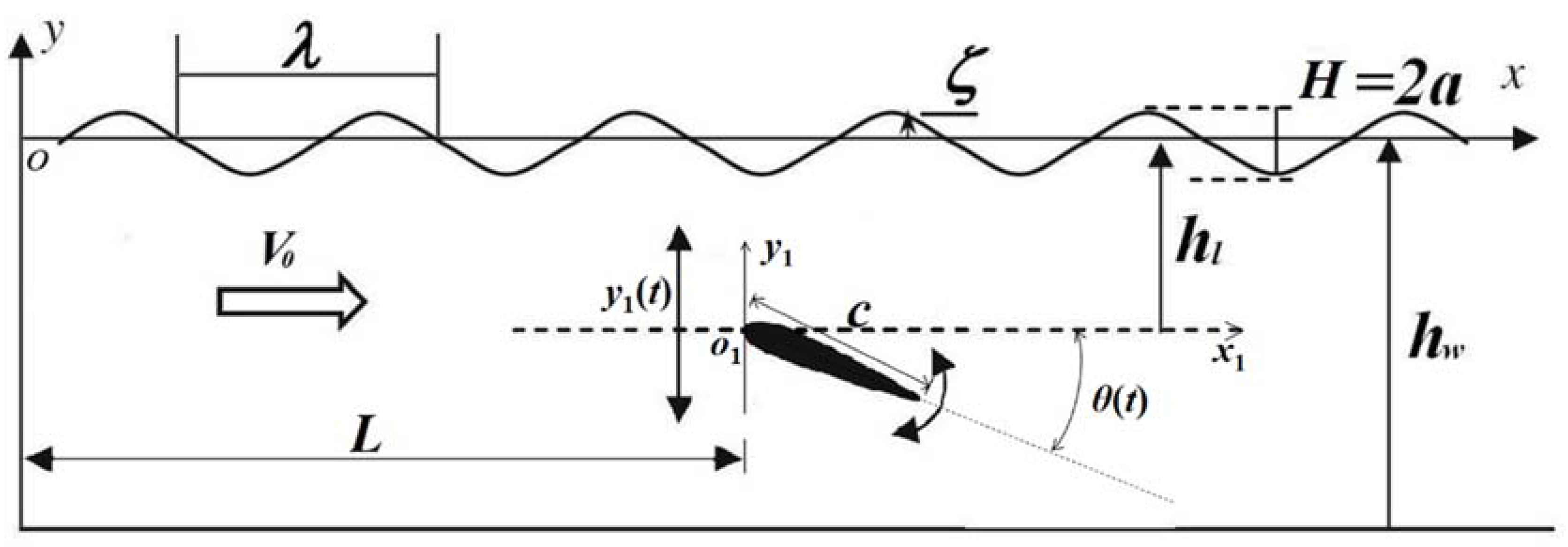
Figure 2.
Schematic diagram of numerical wave tank.
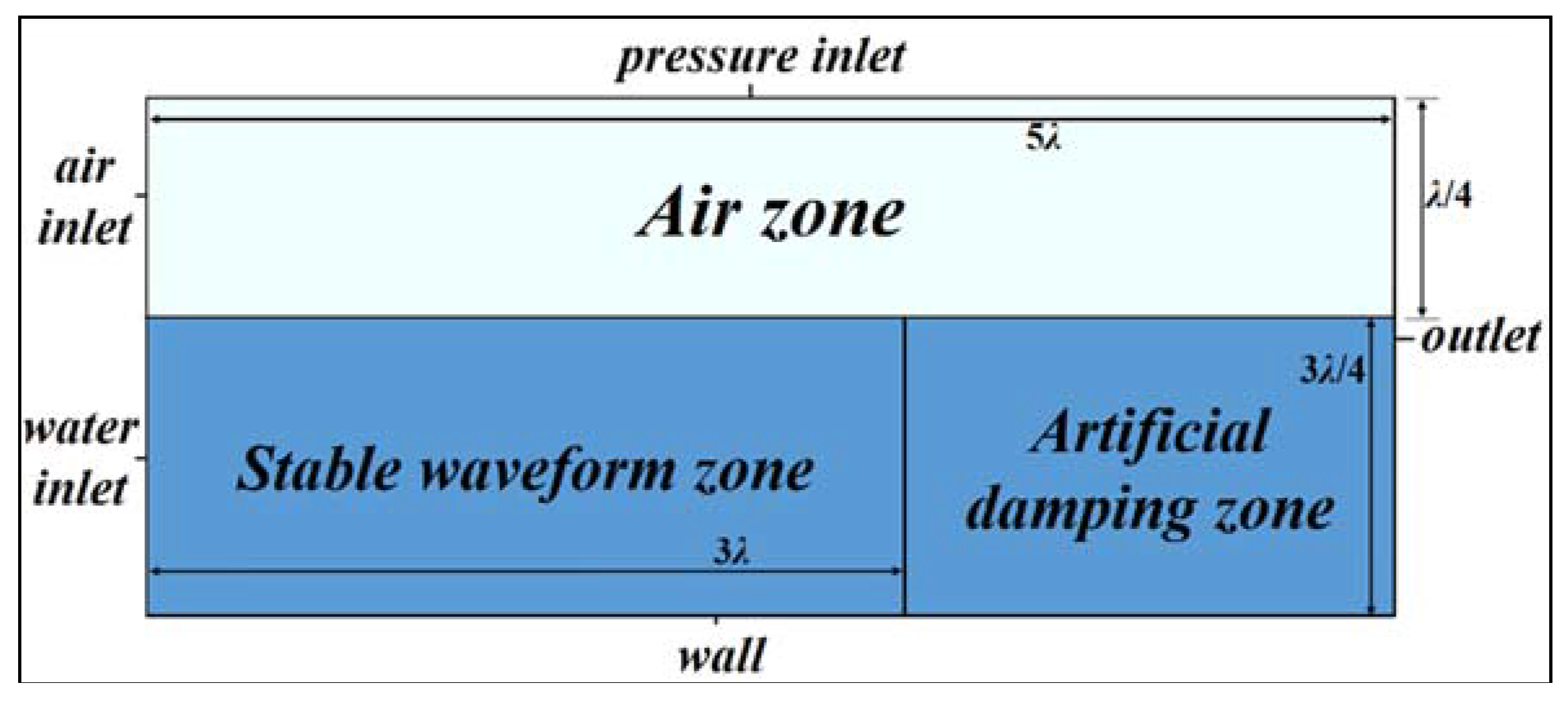
Figure 3.
Schematic diagram of mesh systems.

Figure 4.
The free surface time series at (a) x = 2 m and (b) x = 6 m, and (c) the waveform at t = 20 s.
Figure 4.
The free surface time series at (a) x = 2 m and (b) x = 6 m, and (c) the waveform at t = 20 s.
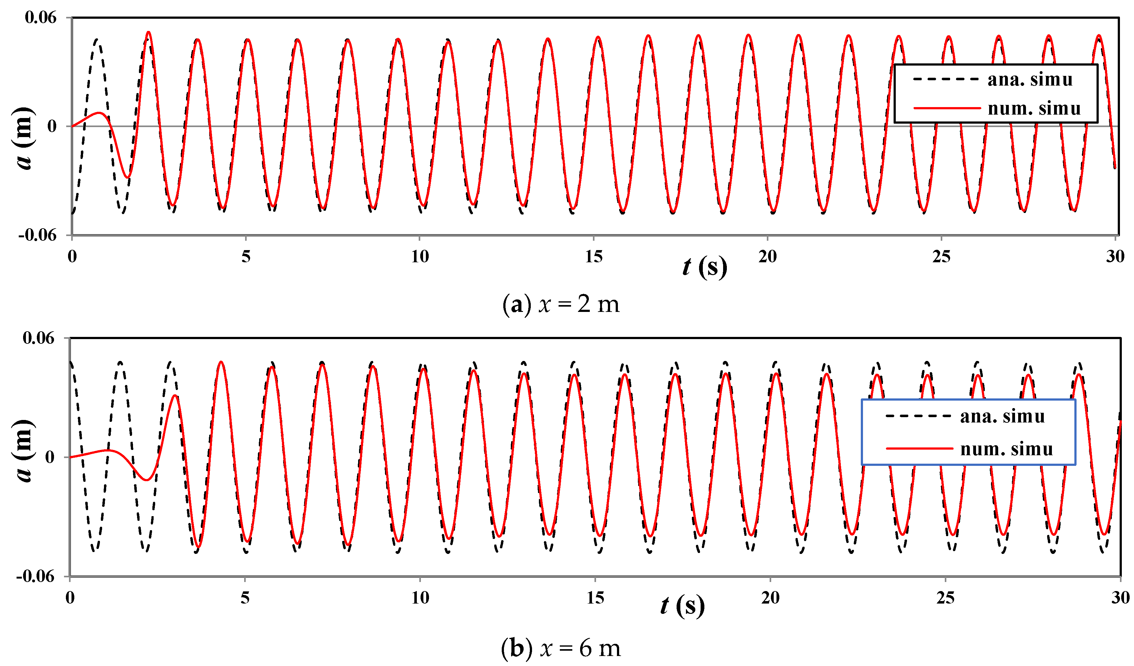

Figure 5.
Comparison of non-dimensional thrust in experiment and theory.

Figure 6.
Average thrust and utilization wave power coefficients for the foil versus wave encounter frequency.
Figure 6.
Average thrust and utilization wave power coefficients for the foil versus wave encounter frequency.
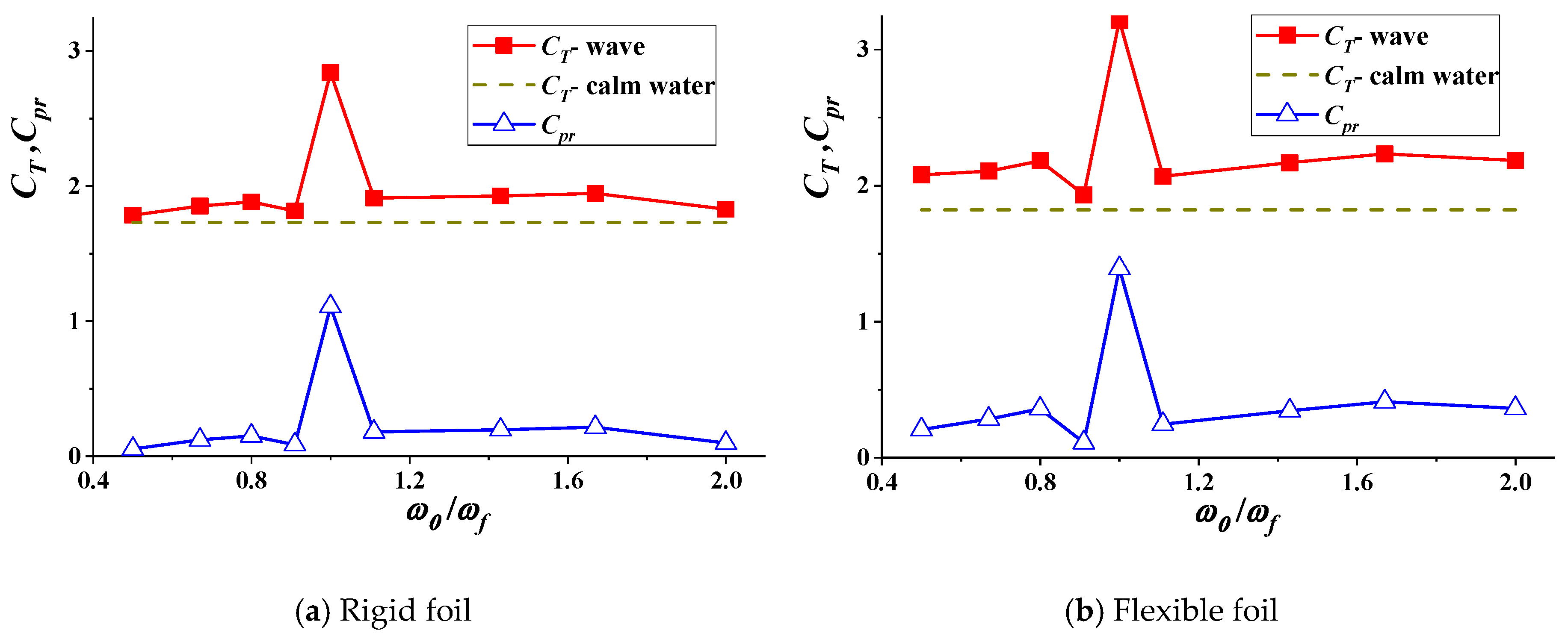
Figure 7.
The percentage of wave energy recovery ηr and propulsive efficiency η for the foil versus wave encounter frequency.
Figure 7.
The percentage of wave energy recovery ηr and propulsive efficiency η for the foil versus wave encounter frequency.

Figure 8.
Average thrust and wave power utilization coefficients for the foil versus non-dimensional wave amplitudes.
Figure 8.
Average thrust and wave power utilization coefficients for the foil versus non-dimensional wave amplitudes.

Figure 9.
The percentage of wave energy recovery ηr and propulsive efficiency η for the foil versus non-dimensional wave amplitudes.
Figure 9.
The percentage of wave energy recovery ηr and propulsive efficiency η for the foil versus non-dimensional wave amplitudes.
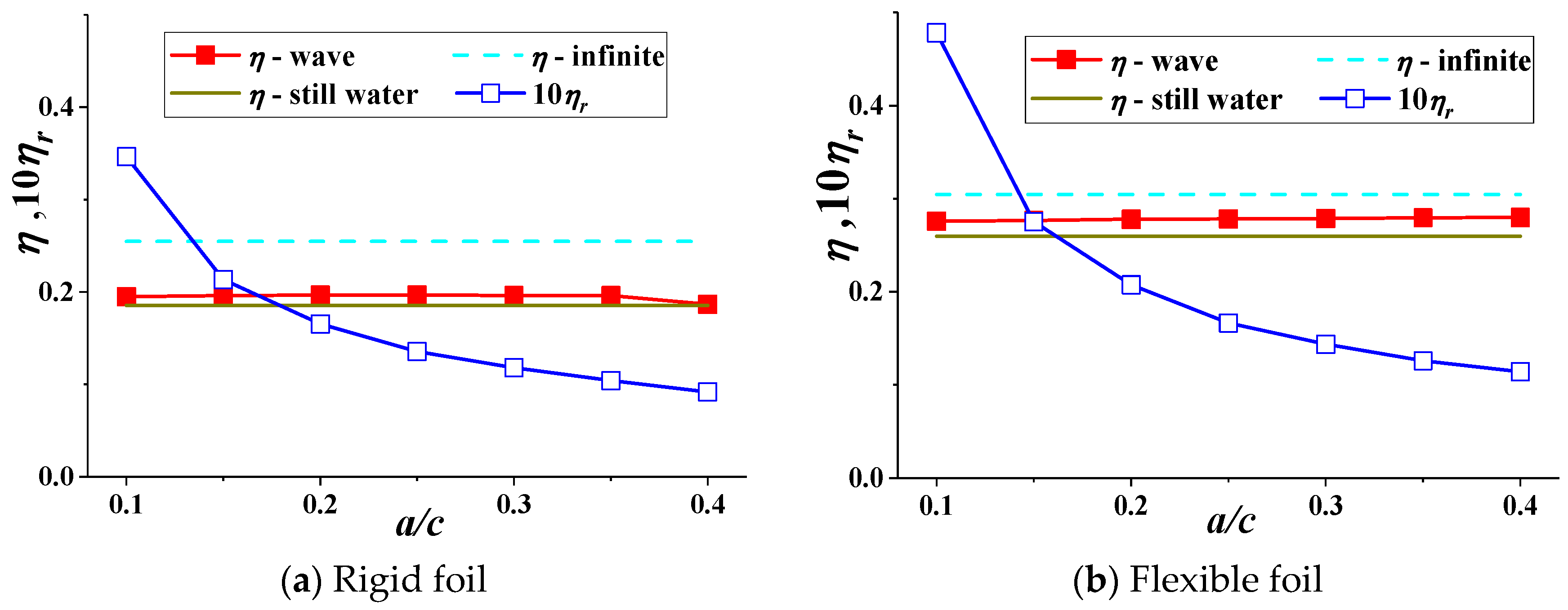
Figure 10.
The average thrust and wave power utilization coefficients for the foil versus non-dimensional wavelengths.
Figure 10.
The average thrust and wave power utilization coefficients for the foil versus non-dimensional wavelengths.

Figure 11.
The percentage of wave energy recovery ηr and propulsive efficiency η for the foil versus non-dimensional wavelengths.
Figure 11.
The percentage of wave energy recovery ηr and propulsive efficiency η for the foil versus non-dimensional wavelengths.

Figure 12.
Dynamic pressure distribution for different wave parameters in one period.
© 2018 by the authors. Licensee MDPI, Basel, Switzerland. This article is an open access article distributed under the terms and conditions of the Creative Commons Attribution (CC BY) license (http://creativecommons.org/licenses/by/4.0/).
Share and Cite
MDPI and ACS Style
Liu, P.; Liu, Y.; Huang, S.; Zhao, J.; Su, Y. Effects of Regular Waves on Propulsion Performance of Flexible Flapping Foil. Appl. Sci. 2018, 8, 934. https://doi.org/10.3390/app8060934
AMA Style
Liu P, Liu Y, Huang S, Zhao J, Su Y. Effects of Regular Waves on Propulsion Performance of Flexible Flapping Foil. Applied Sciences. 2018; 8(6):934. https://doi.org/10.3390/app8060934
Chicago/Turabian StyleLiu, Peng, Yebao Liu, Shuling Huang, Jianfeng Zhao, and Yumin Su. 2018. "Effects of Regular Waves on Propulsion Performance of Flexible Flapping Foil" Applied Sciences 8, no. 6: 934. https://doi.org/10.3390/app8060934
Note that from the first issue of 2016, this journal uses article numbers instead of page numbers. See further details here.