Headphone-To-Ear Transfer Function Estimation Using Measured Acoustic Parameters

1
School of Electronics, Electrical and Communication Engineering, University of Chinese Academy of Sciences, Beijing 100049, China
2
Key Laboratory of Noise and Vibration Research, Institute of Acoustics, Chinese Academy of Sciences, Beijing 100190, China
3
Deng Audio Research, 6350 Willingdon Ave., Burnaby, BC V5H 2V4, Canada
*
Author to whom correspondence should be addressed.
Appl. Sci. 2018, 8(6), 918; https://doi.org/10.3390/app8060918
Submission received: 12 April 2018
/
Revised: 10 May 2018
/
Accepted: 19 May 2018
/
Published: 3 June 2018
(This article belongs to the Section Acoustics and Vibrations)
Abstract
:This paper proposes to use an optimal five-microphone array method to measure the headphone acoustic reflectance and equivalent sound sources needed in the estimation of headphone-to-ear transfer functions (HpTFs). The performance of this method is theoretically analyzed and experimentally investigated. With the measured acoustic parameters HpTFs for different headphones and ear canal area functions are estimated based on a computational acoustic model. The estimation results show that HpTFs vary considerably with headphones and ear canals, which suggests that individualized compensations for HpTFs are necessary for headphones to reproduce desired sounds for different listeners.
1. Introduction
The headphone-to-ear transfer function (HpTF) is defined as the electroacoustic transfer function from the input of a headphone to the sound pressure at the eardrum [1]. In general, HpTFs can be measured by using standard ear simulators on dummy heads. However, current standard ear simulators with fixed acoustic structures cannot simulate the average human ears above 10 kHz and individual differences in ear canal geometry and eardrum impedance [2]. Thus, HpTFs measured by standard ear simulators may not be satisfactory if individual HpTFs over the audible frequency range are needed. It is shown that HpTFs vary considerably with headphones and listeners [3,4]. In the time domain, the impulse response of the HpTF involves the reflections between the inner surface of the headphone and the eardrum. If binaural signals are reproduced through headphones, these reflections interfere with the sound localization cues formed by direction-dependent pinna reflections in the binaural signals, and may cause the front-back confusion in sound localization [5,6]. In the frequency domain, HpTFs introduce timbre distortions [7,8]. Therefore, to faithfully reproduce binaural signals to different listeners through headphones, HpTFs need to be characterized and compensated.
Theoretically, HpTFs should be measured at a point in the ear canal where the binaural signal is recorded [9]. However, direct measurements of individual HpTFs inside human ear canals are difficult and risky. Recently, a method of estimating the HpTF given the headphone acoustic reflectance and equivalent sound source to the ear canal, the ear canal area function and the eardrum impedance has been developed [10]. This means that HpTFs for different headphones and listeners can be estimated through computations based on the parameters of headphones and external ears. In previous studies, there have been some results of the eardrum impedance and reflectance [11] and the ear canal cross-sectional area functions [12,13] measured on human ears. Furthermore, a method for estimating eardrum reflectance and ear canal cross-sectional area functions from ear canal input impedance has also been presented [14]. Thus, in order to estimate the HpTFs for different headphones, the headphone acoustic reflectance and equivalent sound source to the ear canal need to be measured.
The acoustic reflectance of a headphone to the ear canal can be measured by using a single microphone at five measurement positions in an impedance tube sequentially [10]. However, it may be time-consuming to perform sequential measurements if a large number of headphones need to be measured, especially for a wide frequency range with a linear frequency step. To solve this problem, five microphones are simultaneously used to measure the sound pressure signals in the impedance tube [15]. With respect to the determination of the headphone equivalent sound source to the ear canal, some researchers utilize known acoustic impedance as reference loads [16,17]. However, acoustic loads made of long tubes may result in some operation difficulties in the experiments, and the measurement accuracy may be degraded by using the probe microphones as well.
In this paper, an optimal five-microphone array method for measuring the headphone acoustic reflectance and equivalent sound sources needed in the estimation of HpTFs is presented. In contrast to the previous work [15], a compensation function is introduced to compensate the mismatch between microphone sensitivities, and the measurement accuracy of the proposed measurement method is further improved by using a two-stage searching algorithm. The performance of the measurement method is theoretically evaluated and experimentally investigated. With the measured headphone acoustic reflectance and equivalent sound sources, HpTFs for different headphones and ear canal area functions are then estimated through computations based on an acoustic model.
2. The Microphone Array Method for Measuring Acoustic Reflectance
2.1. Theory
For the transfer function method [18,19], two measurement positions are used to measure the reflectance of an acoustic load, and the measurement frequency range is determined by , where is the speed of the sound, and is the distance between the measurement positions. It is clear that two measurement positions cannot achieve satisfactory measurement accuracy over a wide frequency range. Assume microphones located at positions to are simultaneously used in an impedance tube with a pinna simulator, as shown in Figure 1. Let and denote the frequency responses of the incident and reflected sound pressures at , respectively. Then, the output of the nth microphone at position can be expressed as
where is the frequency response of the sensitivity of the nth microphone, is the frequency, is the wave number, and . If tube attenuation is considered, the wave number can be determined as [20]
where is the diameter of the tube.
Considering that different microphones have different sensitivities, this paper introduces a complex compensation function to compensate the mismatch between microphone sensitivities. With the frequency response of the sensitivity of the 1st microphone as reference, the compensation function is defined as
As shown below, the compensation functions can be obtained by calculating the ratio between the frequency response of the 1st microphone and that of the nth microphone measured at the same position in the impedance tube.
Based on Equations (1) and (3), the outputs of N microphones measured at positions to can be written as
Or, in matrix form
where is the output vector of the microphone array, is the matrix of compensation functions, is the propagation matrix determined by the measurement positions, and is the vector containing the unknown incident and reflected sound pressures in the impedance tube. Then, for , the least-squares solution of Equation (5) can be obtained via pseudo-inversion
where is the Hermitian transpose matrix of , and (~) represents the estimated value. With some algebraic manipulations, Equation (6) can be rewritten as
The acoustic reflectance can be determined by
It can be seen from Equation (7) that although is unknown, this term is a common factor that can be cancelled in calculating the ratio between and . Thus, the acoustic reflectance can be calculated from Equation (7) with .
2.2. Error Analysis
In practice, the compensated microphone output signals may contain errors due to the measurement noise and the inaccurate compensation functions. Let the compensated microphone output vector be the sum of the true values and the errors
Then the estimated sound pressure vector can be obtained from Equation (7)
Assume that the elements of are independently distributed with zero mean and equal variance , the expected value of the squared norm of the estimation error can be formulated as
where E[] is the expectation value of a matrix, Tr() is the trace value of a matrix, is the diagonal matrix containing the singular values of , and SF is the singularity factor, defined as [21]
Thus, the sensitivity of the microphone array method to errors caused by measurement noise and inaccurate compensation functions can be evaluated in terms of the SF.
In general, the measurement accuracy of the microphone array method can be improved by increasing the number of microphone positions [22]. However, the effects of measurement accuracy will become marginal when the number of microphone positions is greater than seven [21]. Therefore, to obtain the accurate measurement results with the rational number of microphones, five microphones are chosen in this paper. For the single microphone method [10], where the microphone spacing is , the corresponding SF from 100 Hz to 16 kHz is plotted using the mauve line in Figure 2. In comparison, the SF determined by five microphone positions with uniform spacing of 1.0 cm is plotted using the blue line. As can be seen from Figure 2, the above non-uniform microphone array can achieve a wider effective measurement frequency range than the uniform-spacing configuration, but some fluctuations exist.
The performance of the non-uniform array can be further improved if its SF can be reduced. To do so, a two-staged searching algorithm is presented to find the optimal microphone spacing over the frequency range . Firstly, define the collection of the microphone spacing , i.e.,
where , is the microphone spacing, is the frequency of SF peak within the frequency range, and is the predefined threshold. Then, the optimal microphone spacing can be determined as follows
where , , and is the number of the frequency bins.
To improve the measurement accuracy by optimizing the microphone spacing, the searching algorithm is implemented between two adjacent measurement positions exhaustively at 1 mm step over , where , , , and . The threshold is chosen as 0.85, and the number of the frequency bins is . Among all the configurations, the selected optimal microphone spacing is . The corresponding SF are shown in Figure 2. As can be seen, the optimal microphone positions can lead to an SF with smaller peaks than the previous non-uniform positions. Compared to the above uniform and non-uniform positions, the optimal microphone position has the smallest averaged SF. It is noted that the selected is dependent on the threshold .
3. Experiments
3.1. Measurements of Headphone Acoustic Reflectance
The proposed five-microphone array method is used here to measure the acoustic reflectance for different headphones in a customized impedance tube, which is made of stainless steel with an inner diameter of 8 mm, an outer diameter of 20 mm, and a total length of 380 mm. One end of this tube is connected to a standard small right pinna simulator DB 61 removed from the KEMAR dummy head, and the other end is connected to a sound source (headphone). At the measurement positions, five miniature microphones (Sonion 8002, Suzhou, China) are flush mounted on the tube.
To compensate the microphone mismatch, the frequency responses of all microphones are sequentially measured at position in the impedance tube. The B&K PULSE 3560C (Nærum, Denmark) drives the sound source to produce a linear sweep signal from 20 Hz to 20 kHz. Then the compensation functions in terms of Equation (3) can be determined as
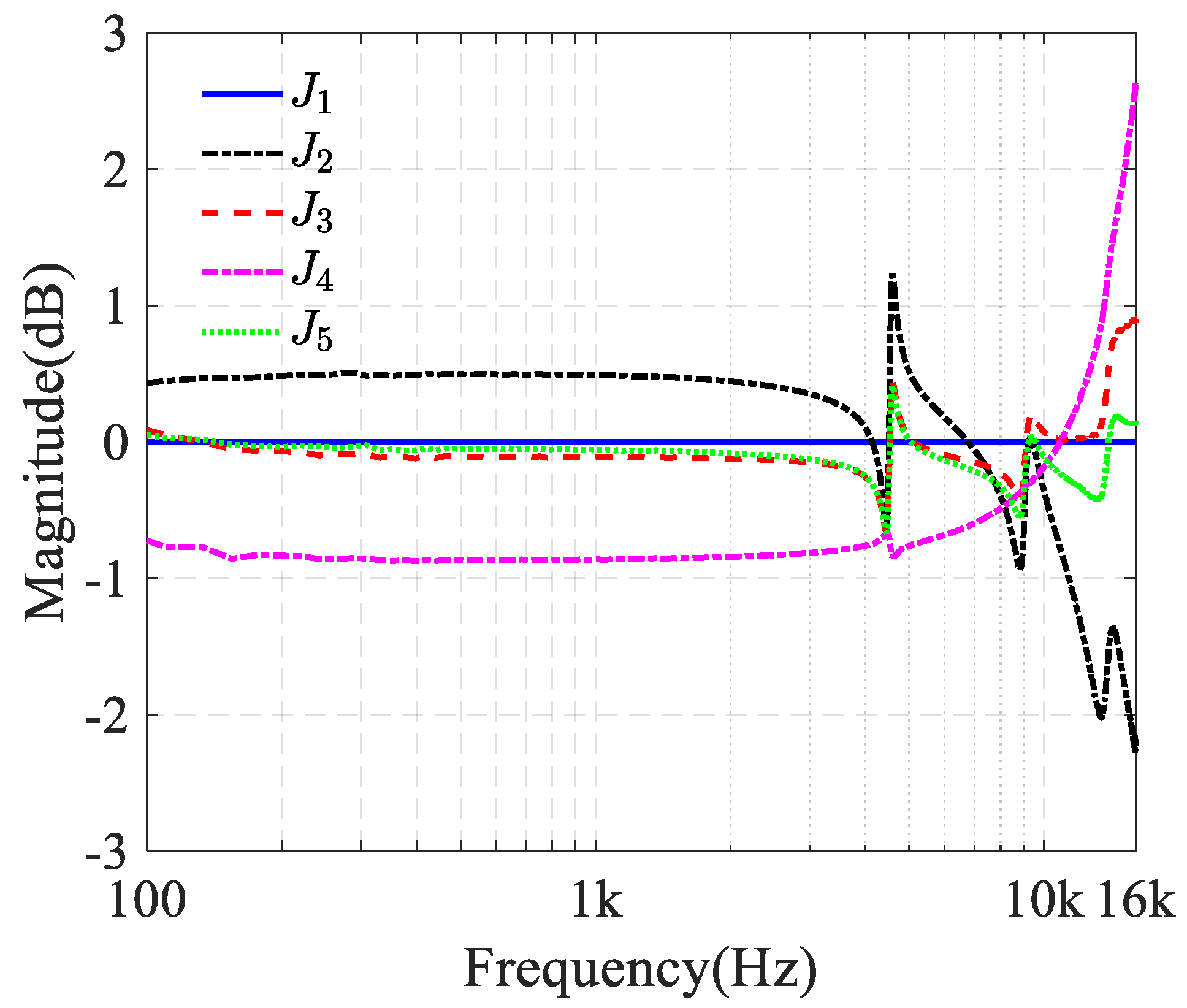
where denotes the frequency response of the nth microphone measured at position . The compensation functions obtained by Equation (15) are shown in Figure 3. After compensation, the five microphones are mounted at the positions to , and the sound source plays the same sweep signal. With the measured compensation functions and sound pressure signals, the headphone acoustic reflectance can be determined by the Equations (7) and (8).
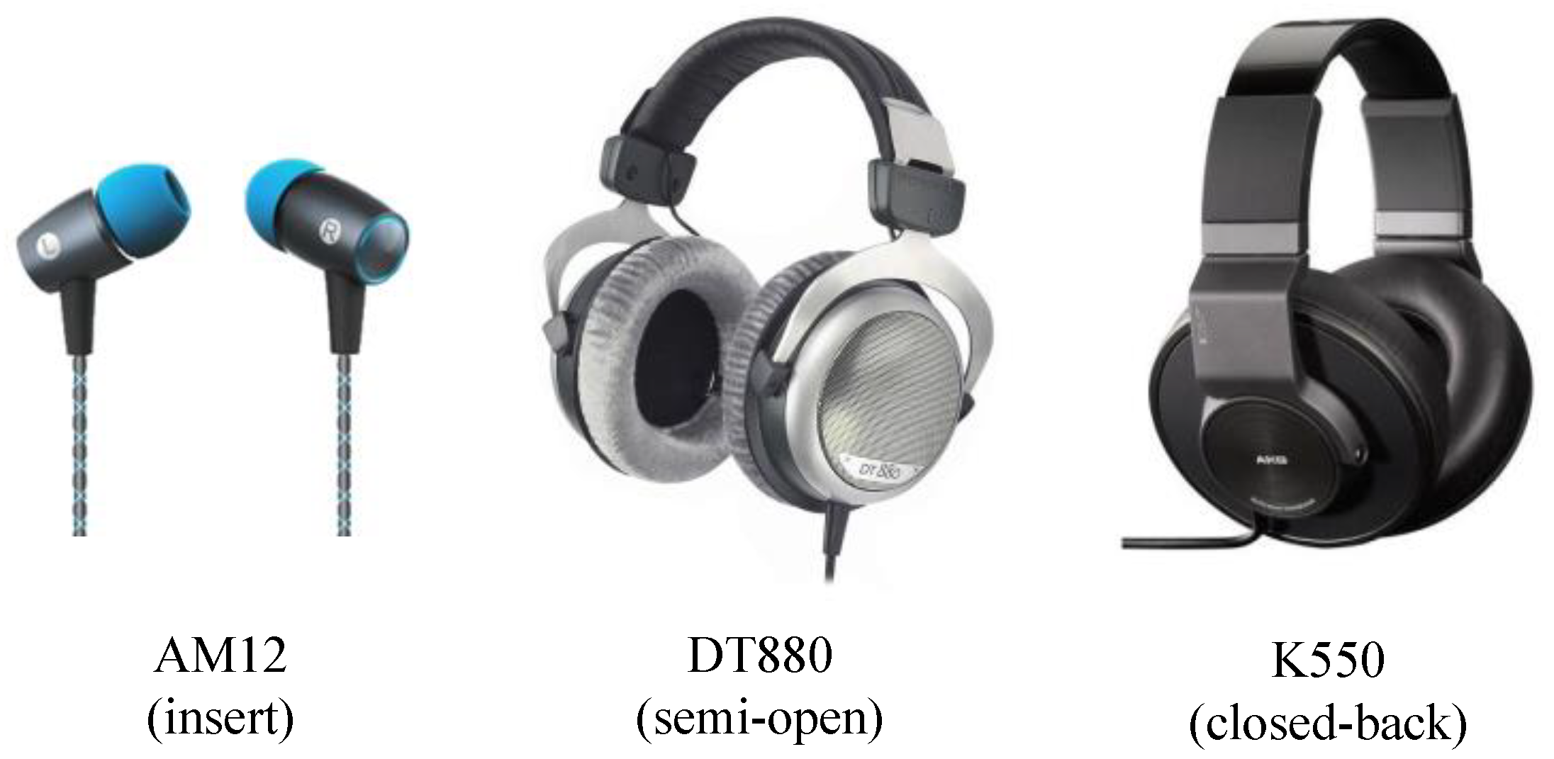
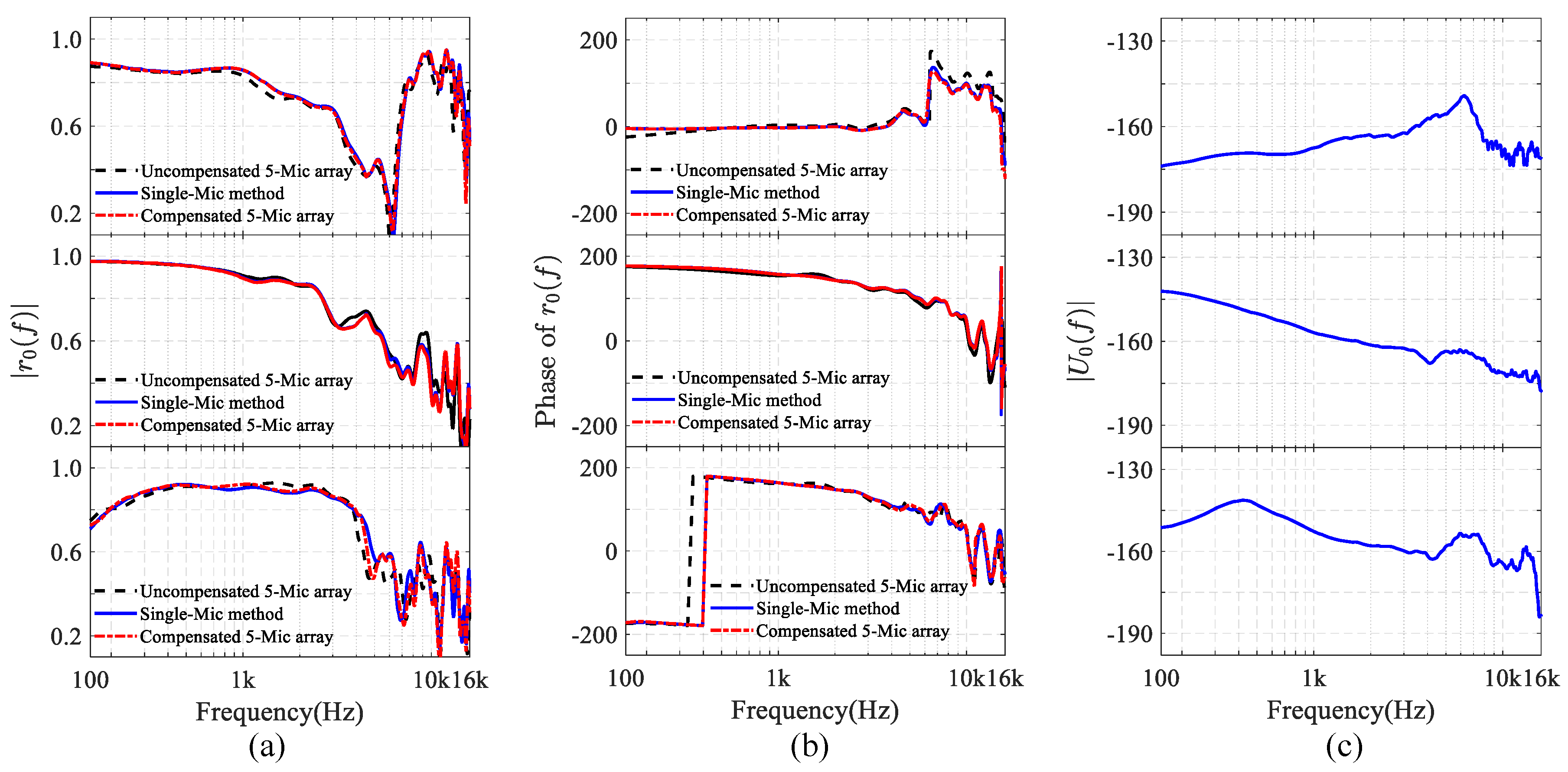
In the experiments, three different types of (insert, semi-open, closed-back) headphones are measured. As shown in Figure 4, the headphone chosen as a representative of each of the headphone type is Huawei AM12 (insert), Beyerdynamic DT880 (semi-open circumaural) and AKG K550 (closed-back circumaural). Figure 5a,b show the magnitude and phase responses of the acoustic reflectance for the above three different types of headphones measured using the proposed five-microphone array method. To validate the proposed method, the magnitude and phase responses of the headphone acoustic reflectance obtained with the single microphone method, which is sequentially measured at each measurement position, are also presented (blue lines) in Figure 5a,b. It can be seen that the results measured by the proposed method are in good agreement with those measured by using the single microphone method, suggesting that the proposed method for accurate measurements of the headphone acoustic reflectance over a wide frequency range is reliable. It should be mentioned that, the measurement results without the compensation function are close to those obtained with the compensation function. This is because the magnitudes of the compensation functions are less than 3 dB, which shows good consistency for all microphones.
3.2. Measurements of Headphone Equivalent Sound Sources
In general, the sound source generated by a headphone to an ear canal can be modeled as the Thevenin equivalent pressure source or the Norton equivalent volume velocity source [16,23]. However, to measure the Thevenin pressure source, the entrance of the ear canal must be physically blocked, which is not feasible for insert headphones. Thus, the Norton equivalent volume velocity source (NEVVS) is used here to characterize the equivalent sound sources of headphones. By using the proposed five-microphone array method, the NEVVSs of different headphones can be measured based on the same impedance tube as used in the measurements of the headphone acoustic reflectance, where the detail measurement steps are described in [10]. The NEVVS responses of the AM12, DT880, and K550 measured by the proposed five-microphone array method are plotted in Figure 5c.
4. Estimation of HpTFs
The human ear canal is about −27 mm long and about 8 mm in diameter, which can be seen as a slightly bended tube with varying cross-sectional areas. In this paper, for simplicity, the acoustic model of the ear canal is approximated as an M-sectional tube with each section having the same length and variable cross-sectional area , and the eardrum impedance is at the end of the Mth section. Given the measured headphone acoustic reflectance and Norton equivalent volume velocity source , the HpTF can be estimated as [10]
where is the wave number in the mth section, , and is the reflectance of the eardrum . To simulate the real human ear, the effective eardrum impedance model [11] and ear canal area function [12] measured on human ears are adopted here for estimating the HpTFs of the Huawei AM12, Beyerdynamic DT880, and AKG K550. The above ear canal area function with fixed ear canal length of 27 mm can be described by the mid locations that refers to the innermost corner of the ear canal and the corresponding radii .
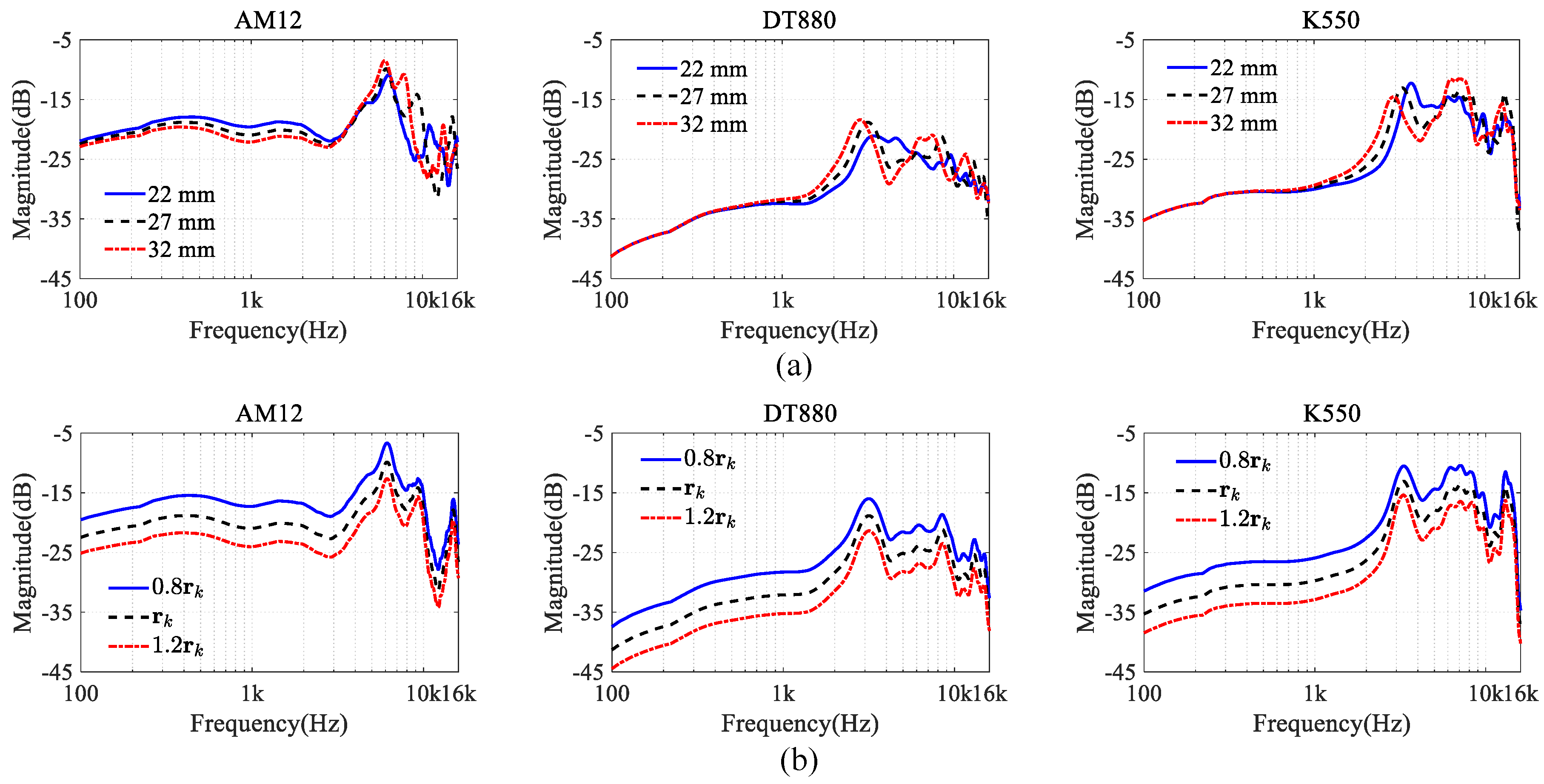
Three different ear canal area functions with fixed and ear canal lengths of 22 mm, 27 mm, and 32 mm, where the corresponding mid locations are , , and are chosen to study the effects of various ear canal lengths on HpTFs, and the estimated HpTFs for the AM12, DT880, and K550 are illustrated in Figure 6a. As can be seen, HpTFs vary considerably with headphones and ear canal lengths. Even for the same headphone, HpTFs show large variations between different ear canal lengths. In particular, for AM12, the peak at 6 kHz is caused by the self-resonance of the headphone, not relying on the length of the ear canal. The difference in HpTFs could be even greater if individual eardrum impedances are taken into account.
In the same way, to study the effects of various ear canal cross-sectional areas on HpTFs, three different ear canal area functions with fixed ear canal length of 27 mm and ear canal radius of , , and are chosen, and the estimated HpTFs for the AM12, DT880, and K550 are depicted in Figure 6b. According to the ear canal acoustic model presented in Equation (16), the effects of the ear canal radii rk on HpTFs can be equivalent to the effects of the eardrum reflectance on HpTFs. As can be seen from Figure 5b, variations of the ear canal radii have a considerable impact on the overall gains of the HpTFs, while the structures of the HpTFs show slight variations. This is because the resonance frequency of the ear canal is mainly dependent on the length of ear canal rather than the eardrum impedance.
On the whole, HpTFs show large variations between different headphones and ear canals. In binaural reproduction, it is desired that individual HpTFs should be compensated in order to faithfully reproduce binaural signals at the eardrums. If compensation using non-individual HpTF from a third person, this may cause considerable perceptual degradation. The method of estimating HpTFs makes it possible to establish a database for various headphones and listeners by adjusting the parameters of headphones and ears. Actual individual eardrum impedances and ear canal area functions are expected to be used in future research.
5. Conclusions
An optimal five-microphone array method is developed for the measurements of the headphone acoustic reflectance and equivalent sound sources needed in the estimation of HpTFs. The optimal microphone positions are selected based on a two-stage searching algorithm, and compensation of microphones is implemented by introducing a compensation function. Experimental results show the effectiveness of the measurement method. This paper proposes that, given the parameters of headphones and ears, HpTFs can be estimated based on a computational acoustic model. The estimation results demonstrate that the parameters of headphones and ear canals have a considerable impact on the HpTFs, and compensations using individual HpTFs are essential for headphone reproduction. Our further research will focus on the effects of individualized compensation using model-based HpTFs on binaural reproduction.
Author Contributions
J.L. and J.Y. conceived the work, and J.L. conducted the experiments. H.D. and P.J. provided suggestions and guidance for the work. J.Y. supervised the project and provided the funding for the experiments.
Acknowledgments
This work was supported by National Natural Science Fund of China under Grants No. 11674348, and Youth Innovation Promotion Association CAS (2015019).
Conflicts of Interest
The authors declare no conflict of interest.
References
- Møller, H. Fundamentals of binaural technology. Appl. Acoust. 1992, 36, 171–218. [Google Scholar] [CrossRef]
- IEC 60318-4. Electroacoustics—Simulators of Human Head and Ear—Part 4: Occluded-Ear Simulator for the Measurement of Earphones Coupled to the Ear by Means of Ear Inserts; International Electrotechnical Commission: Geneva, Switzerland, 2010. [Google Scholar]
- Boren, B.B.; Geronazzo, M.; Majdak, P.; Choueiri, E. PHOnA: A public dataset of measured headphone transfer functions. In Audio Engineering Society Convention 137; Audio Engineering Society: New York, NY, USA, 2014. [Google Scholar]
- Møller, H.; Hammershøl, D.; Jensen, C.B.; Sørensen, M.F. Transfer characteristics of headphones measured on human ears. J. Audio Eng. Soc. 1995, 43, 203–217. [Google Scholar]
- Begault, D.R.; Trejo, L.J. 3-D Sound for Virtual Reality and Multimedia Cambridge; Academic Press Professional: Cambridge, MA, USA, 2000. [Google Scholar]
- Møller, H.; Sørensen, M.F.; Hammershøl, D. Binaural technique: Do we need individual recording? J. Audio Eng. Soc. 1996, 44, 451–469. [Google Scholar]
- Lindau, A.; Brinkmann, F. Perceptual evaluation of headphone compensation in binaural synthesis based on non-individual recordings. J. Audio Eng. Soc. 2012, 60, 54–62. [Google Scholar]
- Schärer, Z.; Lindau, A. Evaluation of equalization methods for binaural signals. In Audio Engineering Society Convention 126; Audio Engineering Society: New York, NY, USA, 2009. [Google Scholar]
- Xie, B. Head-Related Transfer Function and Virtual Auditory Display; J. Ross Pub.: Plantation, FL, USA, 2013. [Google Scholar]
- Deng, H.Q.; Yang, J. Modeling and estimating acoustic transfer functions of external ears with or without headphones. J. Acoust. Soc. Am. 2015, 138, 694–707. [Google Scholar] [CrossRef] [PubMed]
- Shaw, E.A.G. The external ear: New knowledge. Scand. Audiol. Suppl. 1975, 5, 24–50. [Google Scholar]
- Hudde, H.; Engel, A. Measuring and modeling basic properties of the human ear and ear canal. Part III: Eardrum impedances, transfer functions and model calculations. Acust. Acta Acust. 1998, 84, 1091–1108. [Google Scholar]
- Stinson, M.R.; Lawton, B.W. Specification of the geometry of the human ear canal for the prediction of sound-pressure level distribution. J. Acoust. Soc. Am. 1989, 85, 2492–2503. [Google Scholar] [CrossRef] [PubMed]
- Deng, H.Q.; Yang, J. Estimating ear canal geometry and eardrum reflection coefficient from ear canal input impedance. In Proceedings of the 2016 IEEE international conference on Acoustics, Speech and Signal Processing, Shanghai, China, 20–25 March 2016; IEEE: Piscataway, NJ, USA; pp. 251–255. [Google Scholar]
- Liu, J.L.; Deng, H.Q.; Yang, J. A five-microphone method to measure the reflection coefficients of headsets. In Proceedings of the INTER-Noise and NOISE-CON Congress and Conference Proceedings, Hamburg, Germany, 21–24 August 2016. [Google Scholar]
- Hiipakka, M.; Karjalainen, M.; Pulkki, V. Modeling of external ear acoustics for insert headphone usage. J. Audio Eng. Soc. 2010, 58, 269–281. [Google Scholar]
- Keefe, D.H.; Ling, R.; Bulen, J.C. Method to measure acoustic impedance and reflection coefficient. J. Acoust. Soc. Am. 1992, 91, 470–485. [Google Scholar] [CrossRef] [PubMed]
- Cox, T.; D’Antonio, P. Acoustic Absorbers and Diffusers: Theory, Design and Application; CRC Press: Boca Raton, FL, USA, 2016. [Google Scholar]
- Mechel, F.P. Formulas of Acoustics; Springer: Berlin/Heidelberg, Germany, 2008. [Google Scholar]
- International Organization for Standardization (ISO). Acoustics—Determination of Sound Absorption Coefficient and Impedance in Impedance Tubes—Part 2: Transfer-Function Method; ISO 10534-2; International Organization for Standardization: Geneva, Switzerland, 1998. [Google Scholar]
- Jang, S.H.; Ih, J.G. On the multiple microphone method of measuring in-duct acoustic properties in the presence of mean flow. J. Acoust. Soc. Am. 1998, 103, 1520–1526. [Google Scholar] [CrossRef]
- Boden, H.; Abom, M. Influence of errors on the two-microphone method for measuring acoustic properties in ducts. J. Acoust. Soc. Am. 1986, 79, 541–549. [Google Scholar] [CrossRef]
- Voss, S.E.; Allen, J.B. Measurement of acoustic impedance and reflectance in the human ear canal. J. Acoust. Soc. Am. 1994, 95, 372–384. [Google Scholar] [CrossRef] [PubMed]
Figure 1.
The microphone array method for measuring the acoustic reflectance in an impedance tube with a pinna simulator.
Figure 1.
The microphone array method for measuring the acoustic reflectance in an impedance tube with a pinna simulator.
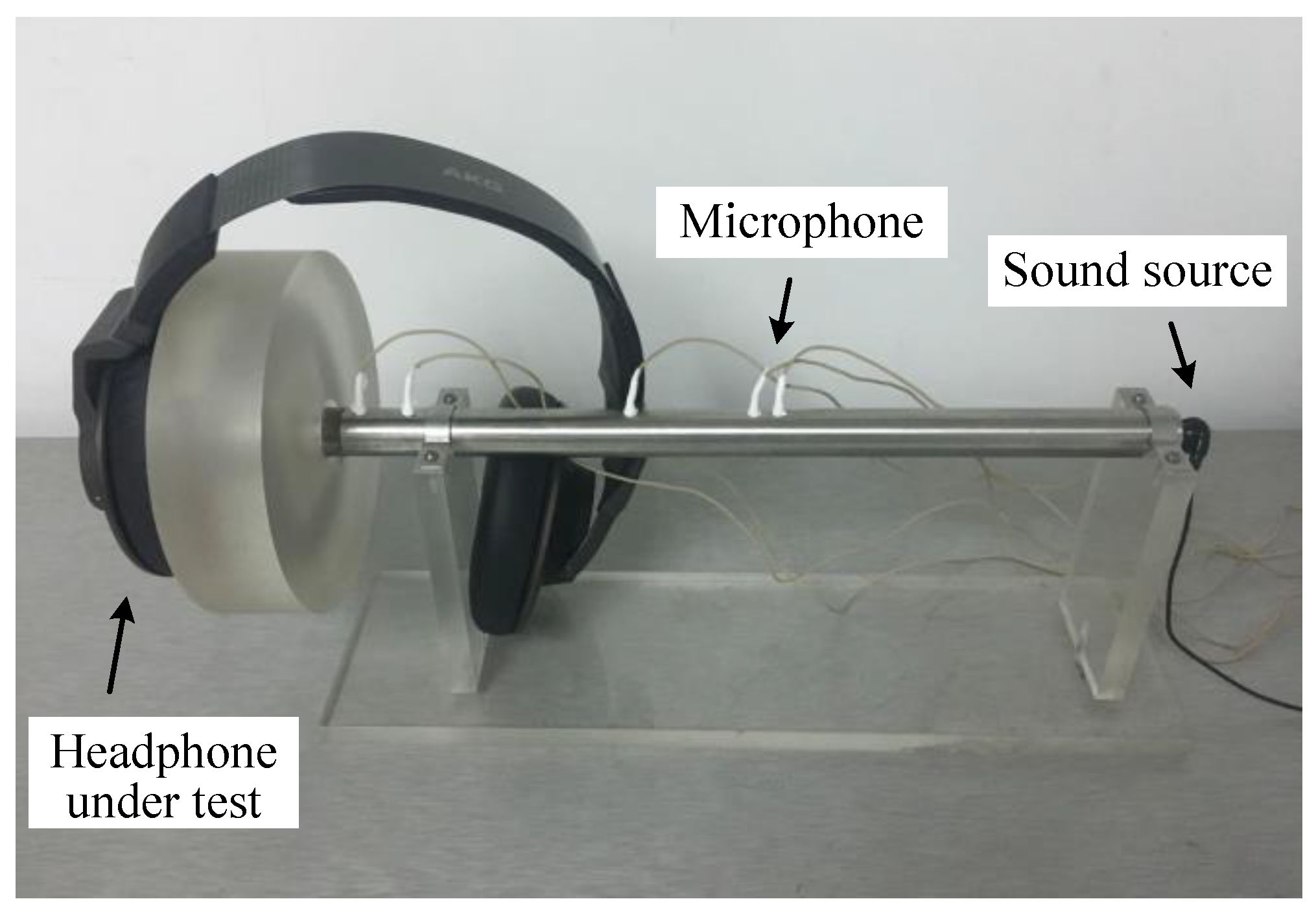
Figure 2.
(Color online) Comparisons of singularity factors determined by the uniform microphone array (blue), the previous five non-uniform microphone array [15] and the optimal microphone array (green).
Figure 2.
(Color online) Comparisons of singularity factors determined by the uniform microphone array (blue), the previous five non-uniform microphone array [15] and the optimal microphone array (green).
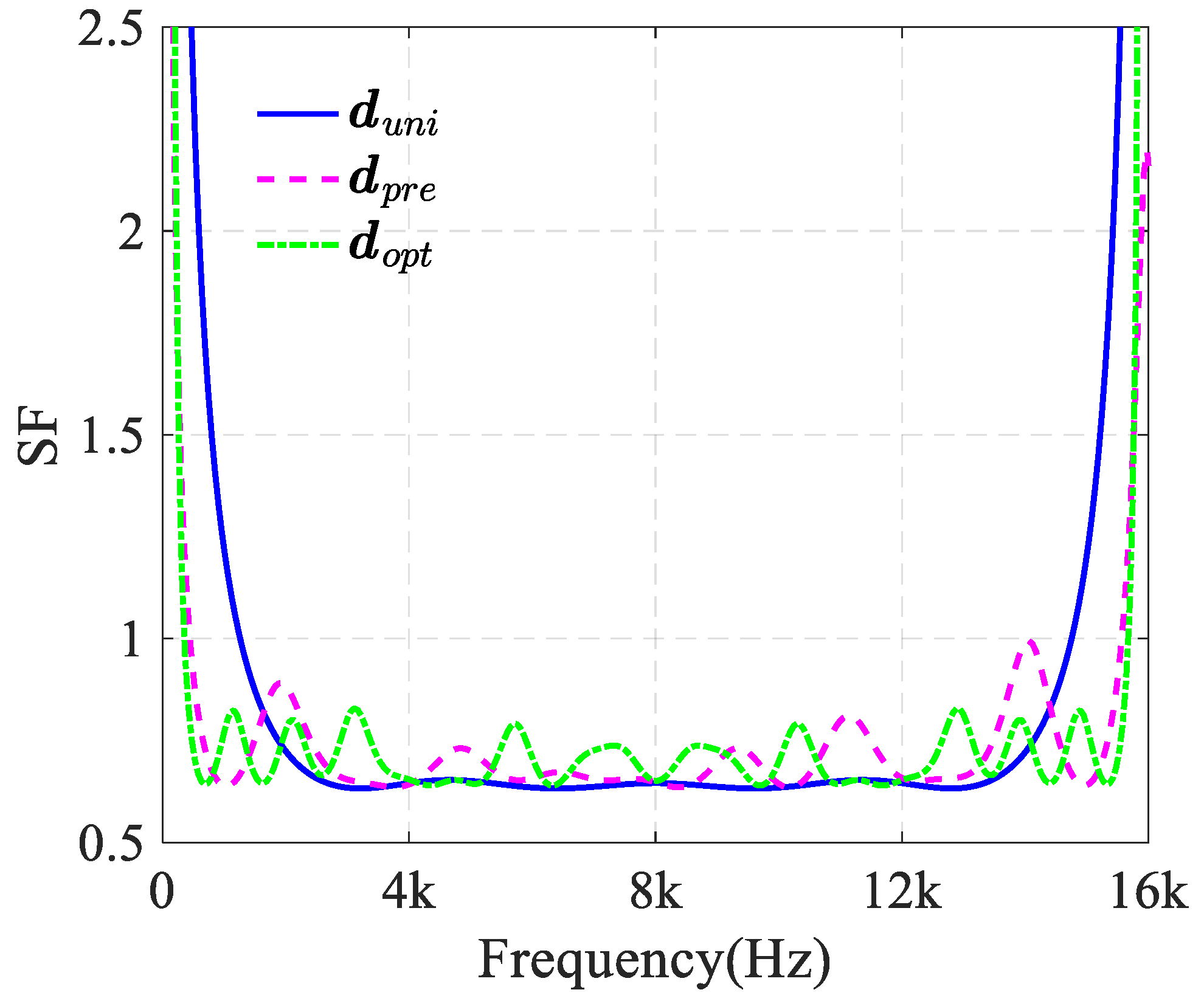
Figure 3.
(Color online) The measured to used for compensating the microphone mismatch in the proposed five-microphone array.
Figure 3.
(Color online) The measured to used for compensating the microphone mismatch in the proposed five-microphone array.

Figure 4.
(Color online) The insert, semi-open and closed-back headphones used in the experiments.

Figure 5.
(Color online) Measurement results of the acoustic parameters for three different types of headphones (First row: Huawei AM12 insert headphone; Second row: Beyerdynamic DT880 semi-open circumaural headphone; Third row: AKG K550 closed-back circumaural headphone). (a) The magnitude responses of the headphone acoustic reflectance; (b) The phase responses of the headphone acoustic reflectance; (c) The magnitude responses of the headphone Norton equivalent volume velocity source (NEVVS).

Figure 6.
(Color online) The estimated HpTFs for three different types of headphones with different ear canal area functions. (a) Ear canal lengths of 22 mm, 27 mm, and 32 mm, respectively; (b) Ear canal radius of (small), (normal), and (large), respectively.
Figure 6.
(Color online) The estimated HpTFs for three different types of headphones with different ear canal area functions. (a) Ear canal lengths of 22 mm, 27 mm, and 32 mm, respectively; (b) Ear canal radius of (small), (normal), and (large), respectively.

© 2018 by the authors. Licensee MDPI, Basel, Switzerland. This article is an open access article distributed under the terms and conditions of the Creative Commons Attribution (CC BY) license (http://creativecommons.org/licenses/by/4.0/).
Share and Cite
MDPI and ACS Style
Liu, J.; Deng, H.; Ji, P.; Yang, J. Headphone-To-Ear Transfer Function Estimation Using Measured Acoustic Parameters. Appl. Sci. 2018, 8, 918. https://doi.org/10.3390/app8060918
AMA Style
Liu J, Deng H, Ji P, Yang J. Headphone-To-Ear Transfer Function Estimation Using Measured Acoustic Parameters. Applied Sciences. 2018; 8(6):918. https://doi.org/10.3390/app8060918
Chicago/Turabian StyleLiu, Jinlin, Huiqun Deng, Peifeng Ji, and Jun Yang. 2018. "Headphone-To-Ear Transfer Function Estimation Using Measured Acoustic Parameters" Applied Sciences 8, no. 6: 918. https://doi.org/10.3390/app8060918
Note that from the first issue of 2016, this journal uses article numbers instead of page numbers. See further details here.