Differential Signalling in Free-Space Optical Communication Systems
by
 , , and
Mojtaba Mansour Abadi
1,*, 
Zabih Ghassemlooy
2,*_Ghassemlooy.jpg) ,
,
Manav R. Bhatnagar
3,
Stanislav Zvanovec
4,
Mohammad-Ali Khalighi
5 and
Martin P. J. Lavery
1 1
School of Engineering, University of Glasgow, Glasgow G12 8LT, UK
2
Faculty of Engineering and Environment, Northumbria University, Newcastle upon Tyne NE1 8ST, UK
3
Department of Electrical Engineering, Indian Institute of Technology Delhi, New Delhi 110016, India
4
Department of Electromagnetic Field, Faculty of Electrical Engineering, Czech Technical University in Prague, 2 Technicka, 16627 Prague, Czech Republic
5
Aix-Marseille University, CNRS, Centrale Marseille, Institut Fresnel, Marseille, France
*
Authors to whom correspondence should be addressed.
Appl. Sci. 2018, 8(6), 872; https://doi.org/10.3390/app8060872
Submission received: 18 April 2018
/
Revised: 14 May 2018
/
Accepted: 18 May 2018
/
Published: 25 May 2018
(This article belongs to the Special Issue Optical Wireless Communications)
Abstract
:In this paper, we review the differential signalling techniques and investigate its implementation of in free-space optical (FSO) communication systems. The paper is an extended version of our previous works, where the effects of background noise, weak turbulence and pointing errors (PE) were investigated separately. Here, for the first time, we present a thorough description of the differential signalling scheme including for combined effects. At first, we present an extension of the analysis of differential signalling to the case of moderate to strong atmospheric turbulence. Next, we investigate a more general case where both channel turbulence and PE are taken into consideration. We provide closed-form expressions for the optimal detection threshold and the average bit-error-rate, and present a set of numerical results to illustrate the performance improvement offered by the proposed differential signalling under various turbulence and PE conditions.
1. Introduction
The received signal in a free-space optical (FSO) communication system is subject to the deterministic and random factors associated with the atmospheric channel, such as geometric loss, particle scattering due to fog, smoke, low clouds, snow, and the influence of the atmospheric turbulence [1,2,3,4,5]. Additionally, pointing errors (PE) due to building sway and thermal expansions can further deteriorate the FSO link performance [6,7,8], whereas fog, smoke, rain, etc. result in a constant power loss; both turbulence and PE lead to random fluctuations of the amplitude and the phase of the received signal. In non-return-to-zero on-off keying (NRZ-OOK) intensity-modulation/direct-detection (IM/DD) based FSO systems, an optimal detection threshold level (DTL) at the receiver (Rx) should be used to distinguish the received ‘0’ and ‘1’ bits [3,4,9]. However, turbulence and PE can result in signal fading [7], which necessitates adaptive setting of the DTL [9]. Recently, a differential signalling scheme (DSS) or differential detection was proposed for on-off keying- (OOK)-based FSO links, which allows using a pre-fixed DTL under various channel conditions such as fog, smoke [9], weak turbulence [3], and PE [4].
Compared to the already proposed detection techniques [10,11,12,13] summarized hereafter, DSS offers the lower complexity of implementation and also does not require the channel state information (CSI). As in [11], a maximum-likelihood sequence detection (MLSD) scheme was proposed for an NRZ-OOK FSO link, and it was shown that provided the temporal turbulence correlation is known, MLSD outperforms the maximum-likelihood symbol-by-symbol detection scheme. However, given that typically ms the proposed MLSD suffers from high computational burden at the Rx, thus making its implementation too complex [14]. To reduce the computational complexity of MLSD, two suboptimal schemes based on the single-step Markov chain model were derived in [12]. However, aforementioned schemes require instantaneous CSI at the Rx. The classical approach for CSI estimation is to periodically insert some symbols in the data frames, which is usually referred to as pilot-symbol assisted modulation (PSAM) [13,15]. The obvious drawback of PSAM is the reduced system throughput due to pilot overhead [13]. A decision–feedback detection scheme was proposed in [16] allowing data detection based on the knowledge of previous decisions within an observation window of . The drawback of this scheme lies in the dependence on and on the data pattern (i.e., bits ‘0’ and ‘1’ in the underlying data stream). The “fast multi-symbol detection” was demonstrated in [10], which works based on block-wise decisions and a fast search algorithm. However, due to the dependency of the system on the search algorithm complexity, there is a trade-off between the throughput and performance of the system. Iterative channel estimation based on the expectation maximization was proposed in [17], but the proposed approach has a relatively high computational complexity. A blind detection scheme requiring no knowledge of CSI as well as the one using a sub-optimum maximum-likelihood detection were introduced in [18,19], respectively. However, these schemes offer rather poor performance over short observation windows. Recently a maximum-likelihood sequence Rx with no knowledge of CSI and channel distribution was proposed in [20] for different channel conditions, which is however too complex to implement.
The DSS investigated in this paper allows performing signal detection without the need to precise setting of DTL in a dynamic FSO channel. Provided that the received differential signals are highly correlated, the DTL of the received differential signal is not influenced by turbulence induced fluctuation [3,4]. Note that, to avoid an adaptive setting of the DTL, high pass filtering (e.g., AC-coupled circuitry) could be a solution, but this will necessitate an increase in the transmit power to compensate for the filter loss and also induces a baseline wander effect [21]. In summary, the main advantages of the DSS technique are: (i) no requirement for CSI or high complexity blind signal detection at the Rx; (ii) no need for a feedback signal to adjust the threshold level; (iii) no pilot overhead and hence on loss in the system throughput; (iv) reducing the adverse effect of background noise at the Rx [22]; (v) mitigation of the effects of the atmospheric channel such as fog and smoke [9], turbulence [3], and PE [4]; and (vii) the use of a single aperture for both FSO links (that ensures high correlation between two FSO channels).
A practically-feasible implementation of DSS with a highly correlated turbulence influenced channel was also proposed in [3]. In [4], we adopted the same concept to mitigate PE induced fading. It was practically shown that DSS was effectively reducing the fluctuations in the DTL of the signal. In addition, a closed-form expression for bit-error-rate (BER) of FSO DSS link with PE was derived and confirmed by simulations. The Monte Carlo technique was used to simulate each case scenario.
This paper presents a considerable extension of our previous results, presenting the closed-form expressions of DTL and BER for an FSO link with both effects of turbulence and PE derived, which have not been reported before. Note that, compared with previous works, in particular [3,4], the original contributions made are: (i) considering a differential signaling technique in correlated channels; (ii) in [3], we only considered weak turbulence, whereas, in this paper, moderate to strong turbulence is investigated; and (iii) in [3,4], turbulence and PE effects were investigated separately, whereas, in this paper, we consider joint effects of both in a FSO link. The work presented here is also different from works of other teams [23,24,25,26], where the joint model of turbulence and pointing errors were presented. In [23,24,25,26], no differential signalling was considered and the analysis reported cannot be applied to the FSO link with differential signalling in correlated channels.
The paper is organised as follows. In Section 2, the concept and theory behind the DSS technique are explained. Section 3 considers the case of the lossy channel as well as the background noise, whereas the influences of weak and moderate to strong turbulence regimes are discussed in Section 4. In Section 5, the channel with PE effect is investigated. The joint influence of turbulence and PE is introduced in Section 6. Section 7 presents an example of numerical results illustrating the performance improvement offered by DSS, and, lastly, Section 8 concludes the paper.
2. Differential Signalling Scheme
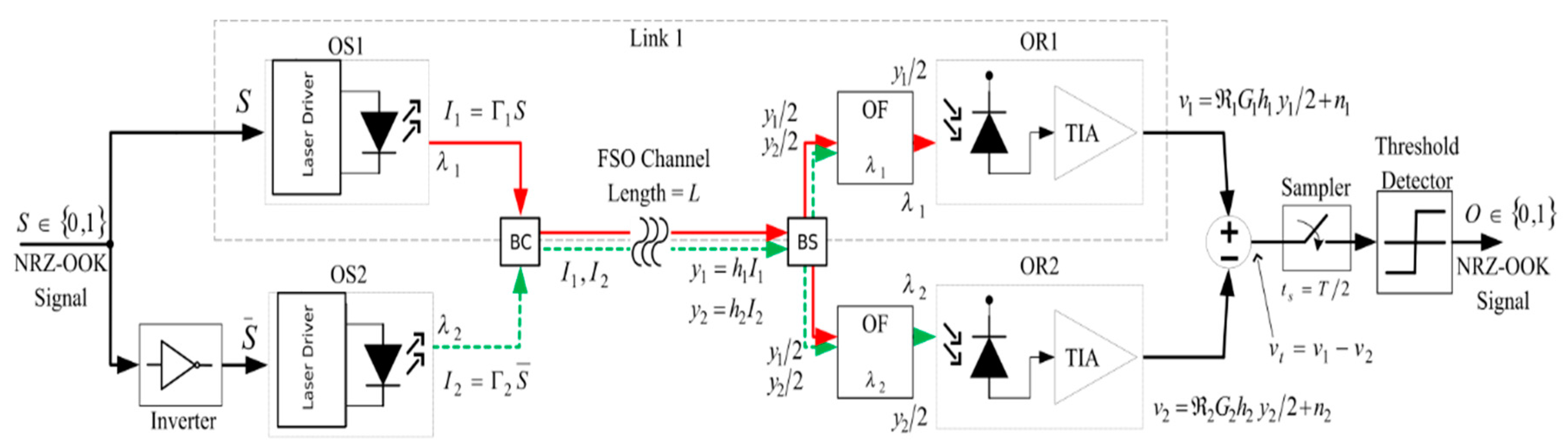
The proposed system block diagram is depicted in Figure 1. The NRZ-OOK signal and its inverted version are used for intensity-modulation of two optical sources at wavelengths of and , respectively. It is worth mentioning that by comparing to the optimal DTL where denotes the expected value, the original data bits (i.e., bit is “0” for and “1” elsewhere) can be retrieved. Note that the optimal DTL for is also . The output intensities () of optical sources (OSs) are given by
where denotes the electrical-to-optical conversion coefficient of i-th OS. Outputs of OSs are then passed through a beam combiner (BC) to ensure that both beams are transmitted over the L-length FSO channel. The optical signals at the Rx are given by
where denotes the channel coefficient (response) including the effects of geometrical and atmospheric losses, PE, and atmospheric turbulence. is passed through a 50/50 beam splitter (BS) and optical filters (OF) with the centre wavelengths of and prior to being collected by an optical Rx. The generated photocurrents are amplified by transimpedance amplifiers (TIA) with outputs given by
where is the photodetector responsivity, is gain of TIA, is the additive white Gaussian noise (AWGN) with zero mean and variance , and denotes the noise power spectral density. The combined output is given by
where . A sampler, sampling at the centre of bit duration, and a threshold detector are used to regenerate the transmit data. From Label (4), the optimal DTL for is given by
For simplicity, we make the following assumptions: (i) links are identical; therefore, we let ; (ii) channels (i.e., transmission path) are very close to each other with and having the same statistical properties, thus being the expected value, where ); and (iii) the chosen wavelengths are close enough to ensure that the channel effects on the propagating optical beams are almost the same. Next, we have [27]
where and are the mean and variance, respectively, and is the correlation coefficient between and . To recover the transmit bit stream, the optimal DTL should be set to the value given by Label (6a), with the variance given in Label (6).
In the electrical domain, is represented by two distinct signal levels of and corresponding to bits “0” and “1”, respectively. For bits, “0” and “1” are recognised as and , respectively. This means that, for the link 1 in Figure 1, the received electrical signals corresponding to bits “0” and “1” are and , respectively. Therefore, the corresponding received differential signals for bits “0” and “1” are and , respectively. Note that the difference between the two bits is twice that of a single link, so without the loss of generality we replace the levels for bits “0” and “1” with and , respectively, and substitute the subtraction of channel responses by , and rewrite Label (4) as
The BER expression for a NRZ-OOK FSO link with an equiprobable data transmission condition is , provided that and are the conditional probabilities given as
where denotes the Gaussian -function defined as , is related to the channel condition, and the electrical signal-to-noise ratio (SNR) = . In the rest of the paper, we will show that, under different channel conditions, in an FSO system with DSS, the average of DTL is always zero and the variance of DTL has the minimum value if the channels are highly correlated. In addition, for highly correlated channels condition, we derive the BER expressions for different channel fading conditions.
3. Lossy Channel and Background Noise
As was mentioned earlier, can represent the total loss in the channel including geometrical loss, fog, or other particle induced scattering. The geometrical loss, which depends on the optical link configuration, is a constant quantity for a fixed point-to-point FSO link. On the other hand, losses due to fog/smoke, which are classified as slow fade events, can be assumed to be relatively constant over the channel for a given time. Under these conditions, both and can be considered constant, and therefore the DTL average and its variance can be determined using Label (6). Note that, since is constant, we can therefore substitute in Label (8) , where is the Dirac delta function. Thus, the averaging integral operation is simplified to the Gaussian -function.
3.1. Geometrical Loss
At the Rx, the received optical beam radius , and the geometrical loss is defined as [28]
where , and are the laser beam radius, beam divergence angle at the transmitter (Tx), respectively. L is the link span and is the aperture diameter at the Rx. Note that, if the maximum Tx lens radius is known, then can be readily determined [29].
3.2. Fog/Smoke Attenuation
The fog loss is determined based on the visibility (Vis) of the channel, which is described by two well-known models of Kim and Kruse [28], and is defined as [30]
where denotes the maximum sensitive wavelength for the human eye, which is normally set to 550 nm (i.e., the green colour). is the wavelength of the laser being used and denotes the loss coefficient. Based on the Kim model, is defined as [31]
The relation between the total loss due to the absorption and scattering of light and loss due to fog is given by the Beer–Lambert law as [31]
Since, for each individual channel, remains constant; therefore, we have and . In addition, based on the assumption we made (i.e., ), the average of DTL from Label (6a) is zero. The total channel coefficient for a DSS based FSO system with geometrical and fog/smoke loss is . Therefore, using Label (9) and Label (12), the channel coefficient can be obtained for determining the BER expressions, which are summarised in Table 1.
3.3. Background Noise
Considering the background noise (i.e., due to sun and artificial lights) [22] the optimal DTL in Label (5) can be reformulated as
Therefore, the variance of DTL in Label (6b) is given as
where is the correlation coefficient between and Using the differential signalling scheme proposed in [22] for the case of using two close wavelengths, here we have and . Assuming the same photodetector parameters at the receiver for the two wavelengths, we have . Under these conditions, the background noise can be effectively rejected after differential detection, and we can obtain the BER formula for the corresponding FSO system with DSS similar to the case in the previous subsection, as presented in Table 1. Note that this BER expression is valid as long as the Rx is not saturated by the ambient light [22].
4. Accounting Atmospheric Turbulence
4.1. Weak Turbulence
In FSO under weak turbulence, the fading of the optical signal can be modelled as , where is a distributed normal random variable (RV) with mean and variance of and , respectively [32]. This way, has a lognormal probability distribution function (PDF) given as [32]
For the log-normal distribution, we have
where [32]; therefore,
where is the correlation coefficient between the turbulence influenced channels. To determine the strength of the turbulence, Rytov variance can be used [33]. For weak turbulence [34], the simplified form of Label (17b) can be used (see Table 1). In the case of a plane wave propagation through a turbulence channel, we have [33]
where is the refractive index structure parameter.
The summation of two lognormal variables can be approximated by a lognormal variable [35,36]; therefore, , where is a Gaussian RV with mean and variance . We will adopt the same procedure as in Wilkinson’s method [35] to estimate the required parameters of . To further normalize , we set the mean value to [27]
where is given by Label (17b) replacing by and letting . Once is determined, it is possible to specify the PDF of a DSS based FSO system using Label (8). The simplified BER expression for weak turbulence is summarised in Table 1. To obtain the closed form equations in weak turbulence, the Gauss–Hermite quadrature formula was used [37]; for details, see Appendix A.
4.2. Moderate to Strong Turbulence
For moderate () to strong () turbulence regimes, we assume , where and refer to large-scale and small-scale atmospheric turbulence effects, respectively [33]. Knowing that both and are expressed by the gamma distribution, we model by the PDF of gamma–gamma (GG) distribution as [38]
where and are also known as the effective numbers of large- and small-scale turbulence cells, respectively [38,39]. , and denote the modified Bessel function of 2nd kind and order , and the gamma function, respectively. The two parameters of a and b characterize the irradiance fluctuation PDF and are related to the atmospheric conditions, which are given by [33]
For the plane wave propagation model and considering the Rx aperture diameter , the closed form expressions for and are given by [33]
where [40]. Knowing that for GG distribution, we have [41,42]
then it is easy to show that
Thus, it is possible to formulate DTL average and variance of the DSS link with the closed-form expression as in Table 1. To derive the BER expression, the Bessel function in Label (20) is replaced with Meijer-G function, which results in simplified BER expression in Table 1. See Appendix A for more details.
5. The Case of Pointing Errors
In a terrestrial FSO link, the joint geometrical loss and PE induced fading within the channel is given by [23]
where , and correspond to beam displacement, the geometrical loss and equivalent beamwidth, respectively. Note that and where and [23]. Note that, if the geometrical loss is taken into account by using Label (9), in Label (25). The PE induced displacement has two major components: (i) the boresight —displacement between the beam centre and centre of the detector; and (ii) jitter —offset of the beam centre at detector plane [24]. The mean offset of PE represents a deviation originated from thermal expansion of buildings [8], whereas is a RV originated from building sway and vibrations [8]. From the statistical point of view, the jitter corresponds to the random variation of the optical beam footprint around the boresight direction with the jitter variance of [43]. It is shown in [8] that in Label (25) has a Rician PDF as below
with the mean and 2nd moment given by
where is the boresight displacement and is the modified Bessel function of the 1st kind with order zero and . Therefore, the variance of is
Substituting Label (27) and Label (28) in Label (6) yields in the DTL average and variance expressions as given in Table 1. Note that we have used to refer to the correlation between PE fading effects within the channels. By using the tail probability of the error events, we can derive the BER for this special scenario where only the PE is considered. The simplified BER expression is outlined in Table 1, whereas detailed derivation for the BER is given in Appendix A.
It is also possible to estimate the equivalent parameters of the DSS based FSO link. For this, we have adopted a single input single output (SISO) link with Rayleigh PE PDF and derived the parameters, which have the same PE variance as DSS. For the simplified case, where , assuming that and , and simplifying , the following equation is derived from which of the equivalent PE PDF as
For , Rician distribution becomes Rayleigh and we assume that the PDF of equivalent PE is also Rayleigh for comparison.
6. Combined Atmospheric Turbulence and Pointing Errors
6.1. Weak Turbulence and PE
The PDF of where is the fading coefficient due to turbulence and represents the effect of PE under log-normal (weak turbulence) channel is given by
where , and . The nth order moment of the above PDF is
and therefore
Therefore, in terms of both ha and hi, Label (32a) is re-written as
Considering the assumption that , similar to the other channel conditions, the average of DTL will be zero. Then, knowing that , is determined using Label (23) and Label (27), which is already given in Label (32b). Finally, using Label (6) and Label (32b), is obtained as given in Table 1. Deriving the expression for the BER in weak turbulence with the presence of PE provides a very complex closed-form expression, which is not convenient to provide here; however, the instruction for a numerical approach to calculate BER is given in Appendix A.
6.2. Moderate to Strong Turbulence and PE
Similar to the weak turbulence regime, the mean and variance for moderate-strong turbulence under the GG channel with the PE are given by
Using Label (6), and Label (34b), is determined as given in Table 1. Deriving the expression for the BER in the moderate to strong turbulence regime with the presence of PE again do not result in a simple closed-form expression, however, the instruction to simplify the numerical approach of BER is given in Appendix A.
Using Label (6), and Label (34b), is determined as given in Table 1. Deriving the expression for the BER in the moderate to strong turbulence regime with the presence of PE again do not result in a simple closed-form expression, however, the instruction to simplify the numerical approach of BER is given in Appendix A.
7. Results and Discussion
In this section, we will present and further discuss the equations derived in the previous section. For each studied case, the variance of DTL as well as the BER of the link is obtained. The wavelengths adopted are 850 and 830 nm and we have assumed that both links have identical parameters. Furthermore, the normalised noise variance is set to 0.06. For the lossy channel and with the ambient light, where channels are inherently highly correlated, the variance of DTL and BER expressions remains the same as under the clear channel condition; therefore, here we focus on the other channel conditions of PE and turbulence. Regarding the series expressions with infinite upper limit in Table 1, it worth mentioning that we did not study the convergence of them. However, we considered between 30–50 terms to calculate the results.
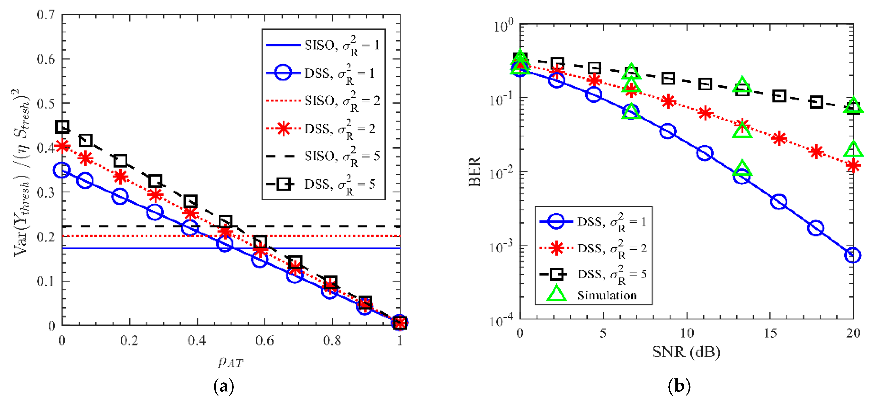
Figure 2 illustrates the results for weak turbulence. The predicted data shown are obtained using the equations given in Section 4.1. Using Label (17b), the predicted normalised variance of DTL against the turbulence for a range of correlation coefficients for SISO and DSS based schemes is shown in Figure 2a. Regardless of turbulence the variance of DTL approaches the minimum value in the cases of highly correlated channels. Note that, on the contrary, the variance of a SISO remains constant, whereas the DSS based scheme offers improved performance at higher turbulence levels. Figure 2b illustrates the BER as a function of SNR for the DSS system for a range turbulence levels. Also displayed are the simulated results, which show a close match with the predicted data. As can be observed, the DSS link, which is assumed to have a high correlation coefficient, display negligible deterioration at higher turbulence levels.
As discussed previously, in the case of moderate to strong turbulence, other models should be adopted to assess the link performance. Here, we have used a GG turbulence model as outlined in Section 6.2 to determine the variance of DTL and the BER of a DSS link as shown in Figure 3. As in the weak turbulence case, for higher levels of turbulence in highly correlated channels, DSS offers improved performance compared with SISO.
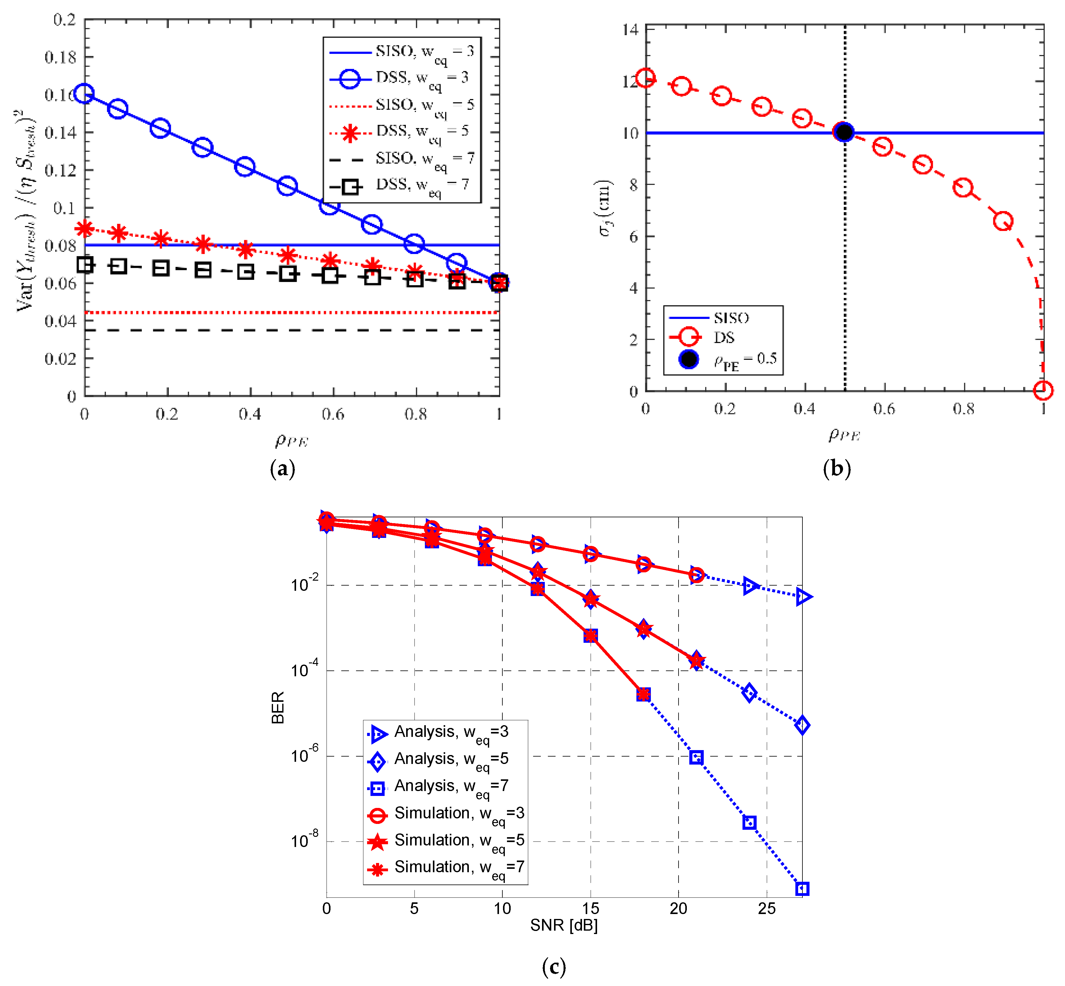
Figure 4a depicts the variance of DTL versus the for both SISO and DSS links for a range of equivalent beamwidth . The plots display the same profile as in Figure 2a with DSS offering improved performance at more significant PE. The benefit of highly correlated DSS compared to the SISO link with the same is more outstanding when reduces. Smaller can be interpreted as the reduced effect of PE on the optical beam. Using the predicted from Label (29), the variance of equivalent DSS PE () can be determined for a range of . Figure 4b depicts the jitter standard deviation against for a SISO link and an equivalent DSS link with , , and . It is observed that the PE induced fading effect reduces with increasing value of . For instance, for an uncorrelated channel with , the normalised variance is ~0.16, whereas, in highly correlated channels, the normalised variance is reduced to ~0.06. Also from both Label (29) and Figure 4b and for we have . The predicted BER results against the SNR for a range of are displayed in Figure 4c showing a good match with the simulated data. Note that, for lower values of the SNR penalty is rather high for a given BER. For instance, at a BER of 10−2, the SNR penalty is ~14 dB for compared . Note that, in Figure 4c, the different SNR vales are obtained by varying the value of noise variance for .
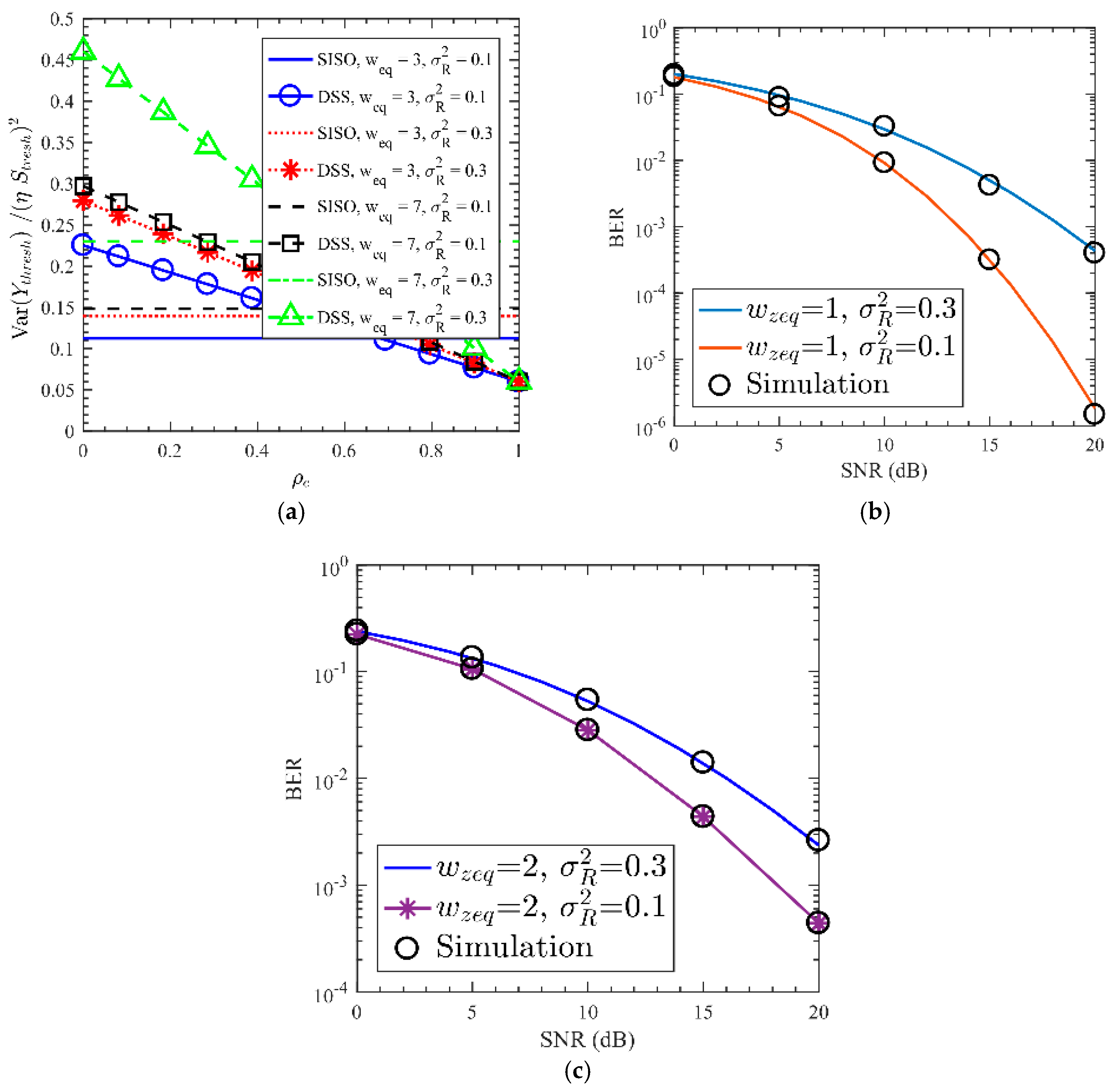
Figure 5a shows the variance of DTL for simultaneous PE and weak turbulence as a function of the channel correlation coefficient for range of 0 to 1. Again, it is seen that, for higher turbulence levels and PE, the DSS system offers improved performance compared to the SISO. The BER versus the SNR for a range of for the combined effects of PE and weak turbulence is plotted in Figure 5b, showing performance degradation at higher levels of turbulence and PE. As expected from Figure 4c, larger improves the BER performance of DSS. Compared to the cases where only turbulence or PE exist in the channel, we observe a significant degradation in the performance. For instance, in a weak turbulence case for and SNR of 10 dB, the BER is less than 10−3. However, for the same turbulence situation, , and SNR of 10 dB, the BER is less than 10−2.
Finally, the combined effects of PE and moderate to strong turbulence on the variance of DTL as well as the BER performance are illustrated in Figure 6a,b, respectively. For these cases, we can observe that even DDS is not mitigating the cannel fading efficiently. Therefore, a designer might consider additional methods such as using a larger aperture to improve the system performance by aperture averaging. The plots show further degradation in both the variance of DTL and the BER compared to Figure 5. The same trend of the larger and the better BER performance of DSS are also seen in Figure 6b. In a strong turbulence regime, PE are less dominant than turbulence. In all variance of DTL plots, one can see that once the channels are highly correlated, the normalised variance of DSS is reduced to the normalised variance of noise with the value of ~0.06. Therefore, under a highly correlated turbulence channel with significant channel fading, it is highly advantageous to implement a DSS FSO scheme in comparison to a SISO one.
8. Conclusions
In this paper, we outlined the essentials of differential signalling based FSO systems subject to the both effects of pointing errors and turbulence. We provided a description comprehensive investigation of the system performance under different conditions of turbulence and/or pointing errors. We derived closed-form expressions for various channel conditions for the DSS based FSO system and showed predicted and simulated results for the variance of DTL and the BER for both SISO and DSS based FSO links. We showed that the DSS based link offers improved performance at higher turbulence and pointing error levels compared to the simple SISO link.
Author Contributions
M.M.A. and M.R.B. carried out the mathematical analysis and simulation; Z.G. and S.Z. proofread and confiremed the analysis; M.-A.K. and M.P.J.L. contributed to the theory material.
Acknowledgments
Portions of this work were presented at the IEEE International Conference on Communications ICC in 2016 (ICC2016), using differential signaling to mitigate pointing errors effect in an FSO communication link. One of the authors, M.M.A. was supported by the PhD studentship from Northumbria University. The work was also supported by the The European project H2020 MSC ITN no. 764461 (VISION) and CTU project SGS17/182/OHK3/3T/13.
Conflicts of Interest
The authors declare no conflict of interest.
Appendix A
A.1. BER Expression in Weak Turbulence
When dealing with the BER expression in weak turbulence in Label (8), the mathematical simplification will result in an expression in the following form:
By substituting , where has a normal random distribution, and setting the integral range, we have
Next, substituting , Label (A2) is re-written as
In Label (A3), can be approximated by Gauss–Hermite quadrature formula as [44], where is the order of approximation, is the zero of the th-order Hermite polynomial, and denotes the th-order weight factor.
A.2. BER Expression in Strong Turbulence
A.3. BER Expression in PE
Let us consider the transmission of the OOK signal, where the received signal can be written corresponding to both states of s as
The decision for the value of is taken by comparing with . Considering two cases of (i) for ; and (ii) for the instantaneous probability of error is given by
By substituting Label (A6a) and Label (A6b) in Label (A7a), we obtain Label (A7b); Label (A7c) is a consequence of the property that , where stands for the probability of . Since , , it can be easily shown that , and the PDF of is given by
From Label (A7), we have
Substituting in Label (A9) and following some algebra, we have
Hence, from Label (A7c), Label (A10), and Label (A11):
Since , therefore, Label (A12) can be rewritten as
The PDF of (unconditional on the instantaneous value of ) under the boresight, PE (i.e., Rician distribution of ) is given by ([8] Equation (5)),
where . For fully correlated and , thus the average BER is given by
Using Label (A14) and the relation , where is the complimentary error function, in Label (A15), we have
where is a natural logarithm function. Employing a substitution and , and following simplifications in Label (A16), we have
where . Let us now use a power series expansion of the complimentary error function
in Label (A17), which results in
Utilizing an identity
in Label (A19) results in the power series based BER expression of the considered scheme.
A.4. BER Expression in Weak Turbulence with PE
The instantaneous BER of the considered scheme is given by Label (A13). The PDF of for weak turbulence with boresight PE is evaluated as
where is given in Label (15) and
In addition,
Since there is no closed-form available of the integral Label (A23), we evaluated this integral using MATLAB (R2016b, US). On substituting the result of Label (A23) into Label (A13), the average BER of the considered system can be obtained.
A.5. BER Expression for Moderate to Strong Turbulence and PE
Similar to weak turbulence with PE, the BER expression under moderate to strong turbulence with PE can be evaluated. Therefore, the PDF of is evaluated as
where and is given in Label (20) and Label (A22), respectively.
In addition,
Integral Label (A25) is determined by numerical integration using MATLAB. Substituting Label (A25) into Label (A13) gives an average BER of the considered system.
References
- Ghassemlooy, Z.; Rajbhandari, S.; Popoola, W. Optical Wireless Communications: System and Channel Modelling with MATLAB; Taylor & Francis: Boca Raton, FL, USA, 2013. [Google Scholar]
- Uysal, M.; Capsoni, C.; Ghassemlooy, Z.; Boucouvalas, A.; Udvary, E. Optical Wireless Communications: An Emerging Technology; Springer: Cham, Switzerland, 2016. [Google Scholar]
- Abadi, M.M.; Ghassemlooy, Z.; Khalighi, M.A.; Zvanovec, S.; Bhatnagar, M.R. FSO detection using differential signaling in outdoor correlated-channels condition. IEEE Photonics Technol. Lett. 2016, 28, 55–58. [Google Scholar] [CrossRef]
- Abadi, M.M.; Ghassemlooy, Z.; Bhatnagar, M.R.; Zvanovec, S.; Khalighi, M.A.; Maheri, A.-R. Using differential signalling to mitigate pointing errors effect in FSO communication link. In Proceedings of the IEEE International Conference on Commuinications ICC’16, Kuala Lumpur, Malaysia, 23–27 May 2016. [Google Scholar]
- Abadi, M.M.; Ghassemlooy, Z.; Zvanovec, S.; Smith, D.; Bhatnagar, M.R.; Wu, Y. Dual Purpose Antenna for Hybrid Free Space Optics/RF Communication Systems. J. Lightw. Technol. 2016, 34, 3432–3439. [Google Scholar] [CrossRef]
- Khalighi, M.A.; Uysal, M. Survey on free space optical communication: A communication theory perspective. IEEE Commun. Surv. Tutor. 2014, 16, 2231–2258. [Google Scholar] [CrossRef]
- Bhatnagar, M.R.; Ghassemlooy, Z. Performance evaluation of FSO MIMO links in Gamma-Gamma fading with pointing errors. In Proceedings of the 2015 IEEE International Conference on, Communications (ICC), London, UK, 8–12 June 2015; pp. 5084–5090. [Google Scholar]
- Fan, Y.; Julian, C.; Tsiftsis, T.A. Free-space optical communication with nonzero boresight pointing errors. IEEE Trans. Commun. 2014, 62, 713–725. [Google Scholar]
- Hitam, S.; Abdullah, M.; Mahdi, M.; Harun, H.; Sali, A.; Fauzi, M. Impact of increasing threshold level on higher bit rate in free space optical communications. J. Opt. Fiber Commun. Res. 2009, 6, 22–34. [Google Scholar] [CrossRef]
- Riediger, M.L.B.; Schober, R.; Lampe, L. Fast multiple-symbol detection for free-space optical communications. IEEE Trans. Commun. 2009, 57, 1119–1128. [Google Scholar] [CrossRef]
- Zhu, X.; Kahn, J.M. Free-space optical communication through atmospheric turbulence channels. IEEE Trans. Commun. 2002, 50, 1293–1300. [Google Scholar]
- Zhu, X.; Kahn, J.M. Markov chain model in maximum-likelihood sequence detection for free-space optical communication through atmospheric turbulence channels. IEEE Trans. Commun. 2003, 51, 509–516. [Google Scholar]
- Zhu, X.; Kahn, J.M. Pilot-symbol assisted modulation for correlated turbulent free-space optical channels. In Proceedings of the SPIE 4489, Free-Space Laser Communication and Laser Imaging, San Diego, CA, USA, 22 January 2002; pp. 138–145. [Google Scholar]
- Xiaoming, Z.; Kahn, J.M.; Jin, W. Mitigation of turbulence-induced scintillation noise in free-space optical links using temporal-domain detection techniques. IEEE Photonics Technol. Lett. 2003, 15, 623–625. [Google Scholar] [CrossRef]
- Xu, F.; Khalighi, A.; Caussé, P.; Bourennane, S. Channel coding and time-diversity for optical wireless links. Opt. Express 2009, 17, 872–887. [Google Scholar] [CrossRef] [PubMed]
- Riediger, M.L.B.; Schober, R.; Lampe, L. Decision-feedback detection for free-space optical communications. In Proceedings of the IEEE 66th Vehicular Technology Conference Fall, Baltimore, MD, USA, 30 September–3 October 2007; pp. 1193–1197. [Google Scholar]
- Dabiri, M.T.; Sadough, S.M.S.; Khalighi, M.A. FSO channel estimation for OOK modulation with APD receiver over atmospheric turbulence and pointing errors. Opt. Commun. 2017, 402, 577–584. [Google Scholar] [CrossRef]
- Riediger, M.L.B.; Schober, R.; Lampe, L. Blind detection of on-off keying for free-space optical communications. In Proceedings of the IEEE Canadian Conference on Electrical and Computer Engineering, CCECE 2008, Niagara Falls, ON, Canada, 4–7 May 2008; pp. 001361–001364. [Google Scholar]
- Chatzidiamantis, N.D.; Karagiannidis, G.K.; Uysal, M. Generalized maximum-likelihood sequence detection for photon-counting free space optical systems. IEEE Trans. Commun. 2010, 58, 3381–3385. [Google Scholar] [CrossRef]
- Tianyu, S.; Pooi-Yuen, K. A robust GLRT receiver with Implicit channel estimation and automatic threshold adjustment for the free space optical channel with IM/DD. J. Lightw. Technol. 2014, 32, 369–383. [Google Scholar]
- Ghassemlooy, Z. Investigation of the baseline wander effect on indoor optical wireless system employing digital pulse interval modulation [optical wireless communications]. IET Commun. 2008, 2, 53–60. [Google Scholar] [CrossRef]
- Khalighi, M.A.; Xu, F.; Jaafar, Y.; Bourennane, S. Double-laser differential signaling for reducing the effect of background radiation in free-space optical systems. IEEE/OSA J. Opt. Commun. Netw. 2011, 3, 145–154. [Google Scholar] [CrossRef]
- Farid, A.A.; Hranilovic, S. Outage capacity optimization for free-space optical links with pointing errors. J. Lightw. Technol. 2007, 25, 1702–1710. [Google Scholar] [CrossRef]
- Borah, D.K.; Voelz, D.G. Pointing error effects on free-space optical communication links in the presence of atmospheric turbulence. J. Lightw. Technol. 2009, 27, 3965–3973. [Google Scholar] [CrossRef]
- Trung, H.D.; Tuan, D.T.; Pham, A.T. Pointing error effects on performance of free-space optical communication systems using SC-QAM signals over atmospheric turbulence channels. AEU Int. J. Electron. Commun. 2014, 68, 869–876. [Google Scholar] [CrossRef]
- Yang, Y.-Q.; Chi, X.-F.; Shi, J.-L.; Zhao, L.-L. Analysis of effective capacity for free-space optical communication systems over gamma-gamma turbulence channels with pointing errors. Optoelectron. Lett. 2015, 11, 213–216. [Google Scholar] [CrossRef]
- Leon-Garcia, A. Probability and Random Processes for Electrical Engineering; Addison-Wesley: Reading, MA, USA, 1989. [Google Scholar]
- Ales, P. Atmospheric effects on availability of free space optics systems. Opt. Eng. 2009, 48, 066001. [Google Scholar]
- Saleh, B.E.A.; Teich, M.C. Fundamentals of Photonics; Wiley: New York, NY, USA; Chichester, UK, 1991. [Google Scholar]
- Ijaz, M.; Ghassemlooy, Z.; Pesek, J.; Fiser, O.; le Minh, H.; Bentley, E. Modeling of fog and smoke attenuation in free space optical communications link under controlled laboratory conditions. J. Lightw. Technol. 2013, 31, 1720–1726. [Google Scholar] [CrossRef]
- Ijaz, M.; Ghassemlooy, Z.; Perez, J.; Brazda, V.; Fiser, O. Enhancing the atmospheric visibility and fog attenuation using a controlled FSO channel. IEEE Photonics Technol. Lett. 2013, 25, 1262–1265. [Google Scholar] [CrossRef]
- Navidpour, S.M.; Uysal, M.; Kavehrad, M. BER performance of free-space optical transmission with spatial diversity. IEEE Trans. Wirel. Commun. 2007, 6, 2813–2819. [Google Scholar] [CrossRef]
- Andrews, L.C.; Phillips, R.L. Laser Beam Propagation through Random Media, 2nd ed.; SPIE Press Monograph; SPIE Publications: Bellingham, WA, USA, 2005; Volume 152. [Google Scholar]
- Hajjarian, Z.; Fadlullah, J.; Kavehrad, M. MIMO free space optical communications in turbid and turbulent atmosphere (Invited Paper). J. Commun. 2009, 4, 524–532. [Google Scholar] [CrossRef]
- Abu-Dayya, A.A.; Beaulieu, N.C. Comparison of methods of computing correlated lognormal sum distributions and outages for digital wireless applications. In Proceedings of the 1994 IEEE 44th Vehicular Technology Conference, Stockholm, Sweden, 8–10 June 1994; Volume 1, pp. 175–179. [Google Scholar]
- Alouini, M.S.; Simon, M.K. Dual diversity over correlated log-normal fading channels. IEEE Trans. Commun. 2002, 50, 1946–1959. [Google Scholar] [CrossRef]
- Stegun, I.A.; Abramowitz, M. Handbook of Mathematical Functions: With Formulas, Graphs and Mathematical Tables; National Bureau of Standards: Washington, DC, USA, 1970.
- Chatzidiamantis, N.D.; Karagiannidis, G.K. On the distribution of the sum of Gamma-Gamma variates and applications in RF and optical wireless communications. IEEE Trans. Commun. 2011, 59, 1298–1308. [Google Scholar] [CrossRef]
- Zixiong, W.; Wen-De, Z.; Songnian, F.; Chinlon, L. Performance comparison of different modulation formats over free-space optical (FSO) turbulence links with space diversity reception technique. IEEE Photonics J. 2009, 1, 277–285. [Google Scholar] [CrossRef]
- Khalighi, M.A.; Schwartz, N.; Aitamer, N.; Bourennane, S. Fading reduction by aperture averaging and spatial diversity in optical wireless systems. IEEE/OSA J. Opt. Commun. Netw. 2009, 1, 580–593. [Google Scholar] [CrossRef]
- Yang, G.; Khalighi, M.A.; Bourennane, S.; Ghassemlooy, Z. Fading correlation and analytical performance evaluation of the space-diversity free-space optical communications system. J. Opt. 2014, 16, 035403. [Google Scholar] [CrossRef]
- Yang, G.; Khalighi, M.A.; Ghassemlooy, Z.; Bourennane, S. Performance analysis of space-diversity free-space optical systems over the correlated Gamma-Gamma fading channel using Pade approximation approximation method. IET Commun. 2014, 8, 2246–2255. [Google Scholar] [CrossRef]
- Borah, D.K.; Voelz, D.; Basu, S. Maximum-likelihood estimation of a laser system pointing parameters by use of return photon counts. Appl. Opt. 2006, 45, 2504–2509. [Google Scholar] [CrossRef] [PubMed]
- Gradshtein, I.S.; Jeffrey, A.; Ryzhik, I.M. Table of Integrals, Series, and Products, 5th ed.; Academic Press: Boston, MA, USA; London, UK, 1994. [Google Scholar]
- Jeffrey, A.; Zwillinger, D. Table of Integrals, Series, and Products; Elsevier Science: Burlington, ON, Canada, 2000. [Google Scholar]
Figure 1.
A schematic block diagram of differential signalling scheme (DSS). The labels OS, BC, BS, OR, OF, and TIA are optical source, beam combiner, beam splitter, optical Rx, optical filter, and transimpedance amplifier, respectively. is the bit duration.
Figure 1.
A schematic block diagram of differential signalling scheme (DSS). The labels OS, BC, BS, OR, OF, and TIA are optical source, beam combiner, beam splitter, optical Rx, optical filter, and transimpedance amplifier, respectively. is the bit duration.

Figure 2.
Single-input single-output (SISO) and differential signaling scheme (DSS) based free-space optical (FSO) links with weak turbulence: (a) the normalised variance of detection threshold level (DTL) versus the correlation coefficient of the channels; and (b) bit-error-rate (BER) against signal-to-noise ratio (SNR) for a range of .

Figure 3.
Single-input single-output (SISO) and differential signaling scheme (DSS) based free-space optical (FSO) links with moderate to strong turbulence: (a) the normalised variance of detection threshold level (DTL) versus the correlation coefficient of the channels; and (b) bit-error-rate (BER) against signal-to-noise ratio (SNR) for a range of .

Figure 4.
Single-input single-output (SISO) and differential signaling scheme (DSS) based free-space optical (FSO) links with pointing errors (PE): (a) the normalised variance of detection threshold level (DTL) versus the correlation coefficient of the channels; (b) the jitter standard deviation of the equivalent DSS PE vs. correlation coefficient , for the SISO system with DSS and for , and , and (c) bit-error-rate (BER) against signal-to-noise ratio (SNR) for , and different values of with unit of .

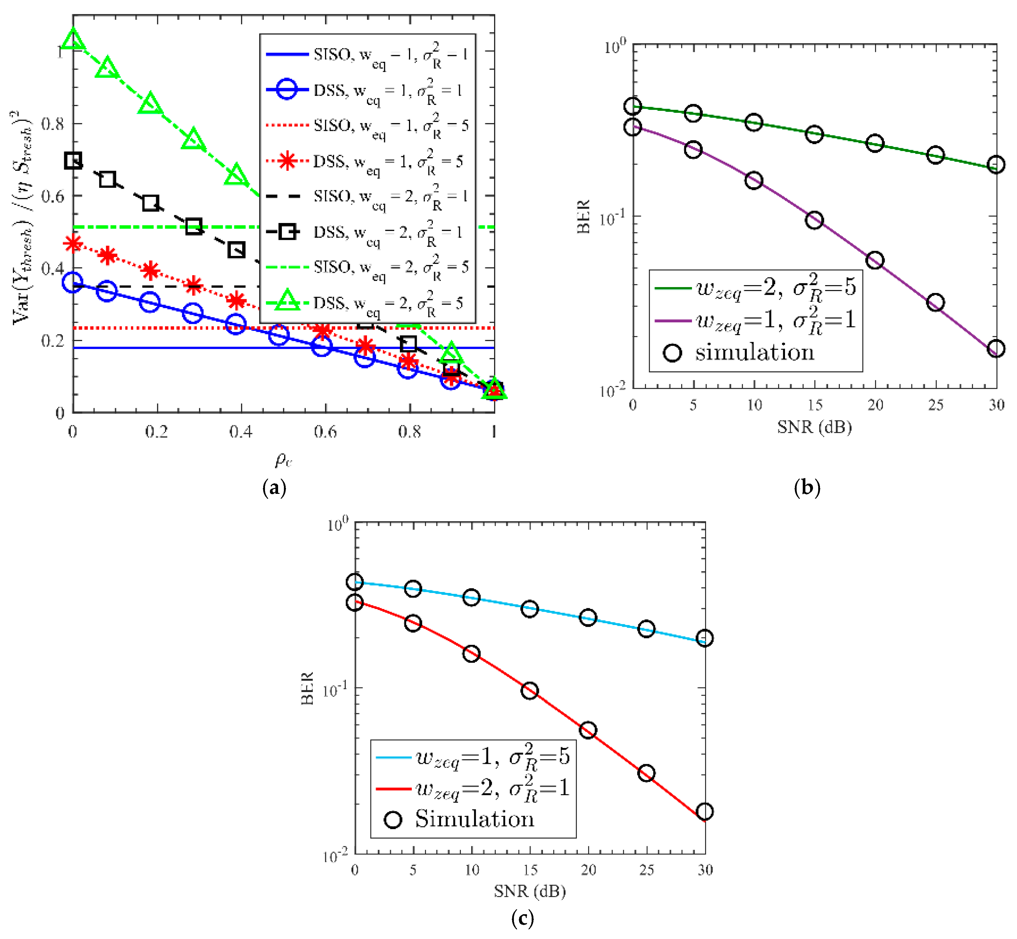
Figure 5.
Single-input single-output (SISO) and differential signaling scheme (DSS) based free-space optical (FSO) links with pointing errors (PE) and weak turbulence: (a) the normalised variance of detection threshold level (DTL) versus the correlation coefficient of the channels; and (b, c) bit-error-rate (BER) against signal-to-noise ratio (SNR) for different values of with unit of and .

Figure 6.
Single-input single-output (SISO) and differential signaling scheme (DSS) based free-space optical (FSO) links with pointing errors (PE) and moderate to strong turbulence: (a) the normalised variance of detection threshold level (DTL) versus the correlation coefficient of the channels; and (b,c) bit-error-rate (BER) against signal-to-noise ratio (SNR) for different values of with unit of and .


Table 1.
Summary of closed-form expressions of the variance of detection threshold level (DTL) and bit-error-rate (BER) for a free space optical (FSO) link under pointing errors under different channel conditions.
Table 1.
Summary of closed-form expressions of the variance of detection threshold level (DTL) and bit-error-rate (BER) for a free space optical (FSO) link under pointing errors under different channel conditions.
| Channel | Variance of DTL, | BER |
|---|---|---|
| Lossy | ||
| Background Noise | ||
| Pointing Errors | , , is the boresight displacement | |
| Weak Turbulence | is obtained by (19). For , and refer to Appendix A. | |
| Moderate to Strong Turbulence | ||
| Weak Turbulence and Pointing Errors | is the combined channel correlation coefficient | Substitute Label (4.3) into Label (3.8) |
| Moderate to Strong Turbulence and Pointing Errors | is the combined channel correlation coefficient | Substitute Label (5.2) into Label (3.8) |
© 2018 by the authors. Licensee MDPI, Basel, Switzerland. This article is an open access article distributed under the terms and conditions of the Creative Commons Attribution (CC BY) license (http://creativecommons.org/licenses/by/4.0/).
Share and Cite
MDPI and ACS Style
Mansour Abadi, M.; Ghassemlooy, Z.; Bhatnagar, M.R.; Zvanovec, S.; Khalighi, M.-A.; Lavery, M.P.J. Differential Signalling in Free-Space Optical Communication Systems. Appl. Sci. 2018, 8, 872. https://doi.org/10.3390/app8060872
AMA Style
Mansour Abadi M, Ghassemlooy Z, Bhatnagar MR, Zvanovec S, Khalighi M-A, Lavery MPJ. Differential Signalling in Free-Space Optical Communication Systems. Applied Sciences. 2018; 8(6):872. https://doi.org/10.3390/app8060872
Chicago/Turabian StyleMansour Abadi, Mojtaba, Zabih Ghassemlooy, Manav R. Bhatnagar, Stanislav Zvanovec, Mohammad-Ali Khalighi, and Martin P. J. Lavery. 2018. "Differential Signalling in Free-Space Optical Communication Systems" Applied Sciences 8, no. 6: 872. https://doi.org/10.3390/app8060872
Note that from the first issue of 2016, this journal uses article numbers instead of page numbers. See further details here.