Fault Detection and Isolation for Redundant Inertial Measurement Unit under Quantization

Abstract

Fault detection and isolation with redundant strapdown inertial measurement unit is critical for ensuring the reliability of the guidance or navigation system in the fields of both aeronautics and astronautics. Although the parity space approach is used widely, it cannot detect the soft fault which affects navigation performance under pulse quantization. This paper develops the three-channel filters to detect the soft fault and conducts theoretical implementation. The constraint conditions of their parameters are explored and the influence of the weight of different ratios is analyzed. The Monte Carlo simulation is carried out in order to verify the validity of the fault detection and isolation method. The simulation results and their analysis provide a theoretical reference for fault detection and isolation with redundant strapdown inertial measurement unit.

1. Introduction

In many aerospace applications, the reliability of an inertial sensor is critically important [1]. Two methods are used to enhance the navigation system’s reliability: one is increasing the precision of a single inertial device, whose convergence, however, is limited; another is integrating multiple inertial sensors (more than three) by using appropriate redundant configurations in order to greatly improve the commonly-used navigation system’s reliability and precision [2]. The Delta 4 rocket of the USA uses two sets of laser strapdown inertial measurement unit (IMU) with the relative-rotation installation. The European Space Agency’s (ESA) Ariane 5 rocket uses two sets of laser gyroscope strapdown IMU with the coaxial installation. Japan’s H-2A rocket uses three orthogonal axes plus an inclined axis configuration of the strapdown IMU. To provide information on redundant measurement and improve the reliability and accuracy of their navigation systems, most of China’s new launch vehicles also use the redundant strapdown IMU; for example, its CZ-6 rocket uses double-eight strapdown inertial sensors, and its YZ-1 rocket uses ten redundant strapdown inertial sensors. However, if an inertial sensor fails during flight, the information on failure to be fused may pollute all of the information on navigation, which is a serious threat to flight safety and harms the navigation system’s performance. For example, the inertial navigation system of China’s CZ-3B rocket failed in 1996. The CZ-3B rocket and the satellite mounted on it were destroyed due to sensor failure and caused huge damage to personnel and property. Therefore, it is necessary to conduct timely and accurate fault detection and isolation (FDI) of the redundant IMU in a rocket.

Many scholars developed the parity space approach (generalized likelihood method [3,4], the optimal parity vector method [5,6,7] and the singular value decomposition (SVD) method [8]) for the fault detection and isolation of redundant IMU, whose difference mainly lies in the decoupling matrix construction method. At present, the scholars’ research mainly focuses on improving the parity space approach in order to enhance the navigation performance of the redundant IMU. For example, Kwang [9] and Lee [10] proposed a new FDI method which is suitable for two faulty sensors based on the extended parity space approach. In 2012, Lee [11] applied the parity space analysis method to principal component analysis (PCA): he used six single-axis gyroscopes along the conical surface of a strapdown inertial navigation system (SINS), but this method cannot detect soft fault (small magnitude, which affects navigation performance) successfully. Seung [12] used the parity equation and the discrete wavelet transform of the hybrid fault detection method for an unmanned aerial vehicle’s (UAV) inertial navigation sensors, which achieved good detection results. Élcio [13] proposed a fault detection method based on PCA and SVD mainly for minimal-redundancy systems, which divide FDI into two parts and achieves good results on the low-level and step-biased fault. Zhang [14] found that the decoupling matrix vector of the optimal parity method is linearly relevant and leads to a high false alarm rate. To reduce the high false alarm rate and high isolation error rate of the SVD method presented in [8], Wen [15] improved the decoupling matrix construction method with the parity vector unit, obtaining a lower false alarm rate.

However, the existing approaches cannot detect soft fault correctly after quantization. The angle increment is converted into the number of pulses of the laser gyroscope which has a measurement output. This output is not a real angular velocity but rather the angular increment of the sampling period and the quantization value of the pulse. Similarly, the accelerometer’s output is not a real-time apparent acceleration but the sampling period of the speed increment and its quantization value. The quantization of the laser gyroscope and the accelerometer may disturb the error structure of the original information and bring many transient errors for low maneuvers, which may cause difficulty in fault detection. Yi [16] only introduced the low-pass filter concept and combined the generalized likelihood test (GLT) method for fault diagnosis.

To date, no researchers have put forward a perfect filtering method and theoretically analyzed the FDI of redundant strapdown inertial measurement unit (RIMU). This paper developed the three-channel filters and conducted their theoretical implementation. The method can be utilized well in micro-grid applications such as faults in solar and wind systems [17,18,19,20,21]. The paper proposed the constraint conditions of their parameters and analyzed the performance of the weight of different ratios. Thus, this paper is organized as follows: Section 2 provides a theoretical background to the parity space approach, analyzes the existing problems and presents the constraint conditions of parameters of three-channel filters. Section 3 gives simulation results and their analysis. Section 4 presents the conclusions.

2. Materials and Methods

2.1. Quantization Analysis

2.1.1. The Parity Space Approach

A RIMU usually has more than three inertial sensors (such as a rate gyroscope, accelerometer and magnetometer). This paper mainly focuses on the IMUs of at least five inertial sensors for fault detection and isolation. A measurement equation is defined as follows:

$$\mathit{Z}=\mathit{H}\mathit{X}+\mathit{\epsilon },$$

(1)

where $\mathit{\epsilon }\in {\mathit{R}}^{n\times 1}$ is the measurement noise vector, which satisfies $E\left(\mathit{\epsilon }\right)=0$ and $E\left(\mathit{\epsilon }{\mathit{\epsilon }}^T\right)={\sigma }^2\mathit{I}$. $n$ is the number of gyroscopes. $\mathit{H}\in {\mathit{R}}^{n\times 3}$ is the observation matrix defined by the installation structure of the RIMU. $\mathit{X}\in {\mathit{R}}^{3\times 1}$ is the information on inertial state. $\mathit{Z}\in {\mathit{R}}^{n\times 1}$ is the measurement. We define the decoupling matrix $\mathit{V}$, which satisfies the following conditions:

$$\mathit{V}\mathit{H}=\mathit{0},$$

(2)

$$\mathit{V}{\mathit{V}}^T={\mathit{I}}_{n-3},$$

(3)

$${\mathit{V}}^T\mathit{V}={\mathit{I}}_n-\mathit{H}{\left({\mathit{H}}^T\mathit{H}\right)}^{-1}{\mathit{H}}^T,$$

(4)

Only the decoupling matrix $\mathit{V}$ satisfies the above expressions. We can use the observation matrix and the Potter [22] algorithm to solve the decoupling matrix. They suggest that the decoupling matrix $\mathit{V}$ should be the upper triangular matrix that has the right diagonal elements and that its orthogonalization can fully determine its elements. The details of Potter’s algorithm are as follows:

$$\begin{gathered} \mathit{W}=\mathit{I}-\mathit{H}{\left({\mathit{H}}^T\mathit{H}\right)}^{-1}{\mathit{H}}^T, \\ {\mathit{V}}^2\left(1,1\right)=\mathit{W}\left(1,1\right), \\ \mathit{V}\left(1,j\right)=\mathit{W}\left(1,j\right)/\mathit{V}\left(1,1\right), j=2,\dots ,m \\ {\mathit{V}}^2\left(i,i\right)=\mathit{W}\left(i,i\right)-{\displaystyle \sum _{k=1}^{i-1}}{\mathit{V}}^2\left(k,i\right), i=2,\dots ,\left(m-n\right), \\ \mathit{V}\left(i,j\right)=\left[\mathit{W}\left(i,j\right)-{\displaystyle \sum _{k=1}^{i-1}}\mathit{V}\left(k,i\right)\mathit{V}\left(k,j\right)\right]/\mathit{V}\left(i,i\right), i=2,\dots ,\left(m-n\right) \\ j=\left(i+1\right),\dots ,m, \\ \mathit{V}\left(i,j\right)=0, i=2,\dots ,\left(m-n\right), j=1,\dots ,\left(i-1\right), \end{gathered}$$

(5)

With the decoupling matrix $\mathit{V}$, the following linear independent parity equation set can be obtained: $\mathit{p}=\mathit{V}\mathit{Z}$, where $\mathit{p}$ is the parity vector. We define the detection function as follows:

$$D{F}_d={\mathit{p}}^T{(\mathit{V}{\mathit{V}}^T)}^{-1}\mathit{p},$$

(6)

If $D{F}_d>T_d$, then we decide that a fault occurs.

If $D{F}_d\le T_d$, then we decide that no fault occurs.

Here, $T_d$ is the time-varying threshold value set beforehand by the Monte Carlo method. For example, we generate 100 detection judgment sequences based on digital flight trajectory without fault. For each sampling time, we arrange the values from small to large and the (100-$\zeta$)th data is the threshold when a false alarm rate $\zeta$ is given. After a fault is detected, the fault isolation function is needed and defined as follows:

$$DF{I}_j=\frac{{({\mathit{p}}^T{(\mathit{V}{\mathit{V}}^T)}^{-1}{\mathit{V}}_j)}^2}{{\mathit{V}}_j^T{(\mathit{V}{\mathit{V}}^T)}^{-1}{\mathit{V}}_j},$$

(7)

where ${\mathit{V}}_j$ is the $j$th column of the decoupling matrix $\mathit{V}$. We calculate $DF{I}_j$ ($j=1,2,\dots m$) to find out the maximum $DF{I}_j$, for example, $DF{I}^k{}_j$. Then, we assume that the $k$th sensor has a fault.

2.1.2. Problem Brought by Quantization

The output of the laser IMU is the number of quantized pulses; the quantization process is shown in Figure 1. The measurement $\mathit{Z}$ is divided by the equivalent pulse $\Delta$, which is the numerical value of the angular velocity corresponding to one pulse. The integer part is the measurement output $Q$, and the remainder part accumulates to the next sampling period. The error between $Q\times \Delta$ and $\mathit{Z}$ is the quantization error. Taking a gyroscope as an example, the pulse equivalency is set to 1″ (4.8 × 10⁻⁶ rad) and the sampling period T is 20 ms. When the angular increment in the sampling period is less than one pulse equivalent, the output of the cycle would be 0. The angular increments within the k period would be accumulated to the k + 1 cycle for outputting. The output of pulse equivalency is equal to pulse equivalency 1″/T = 50°/h in the sample period. That is to say, after quantization, the instantaneous error is likely to be more than 50 times, which would cause great difficulties in fault detection.

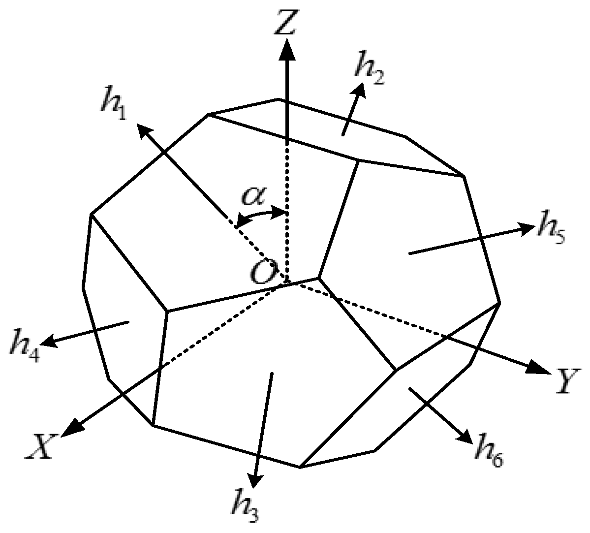
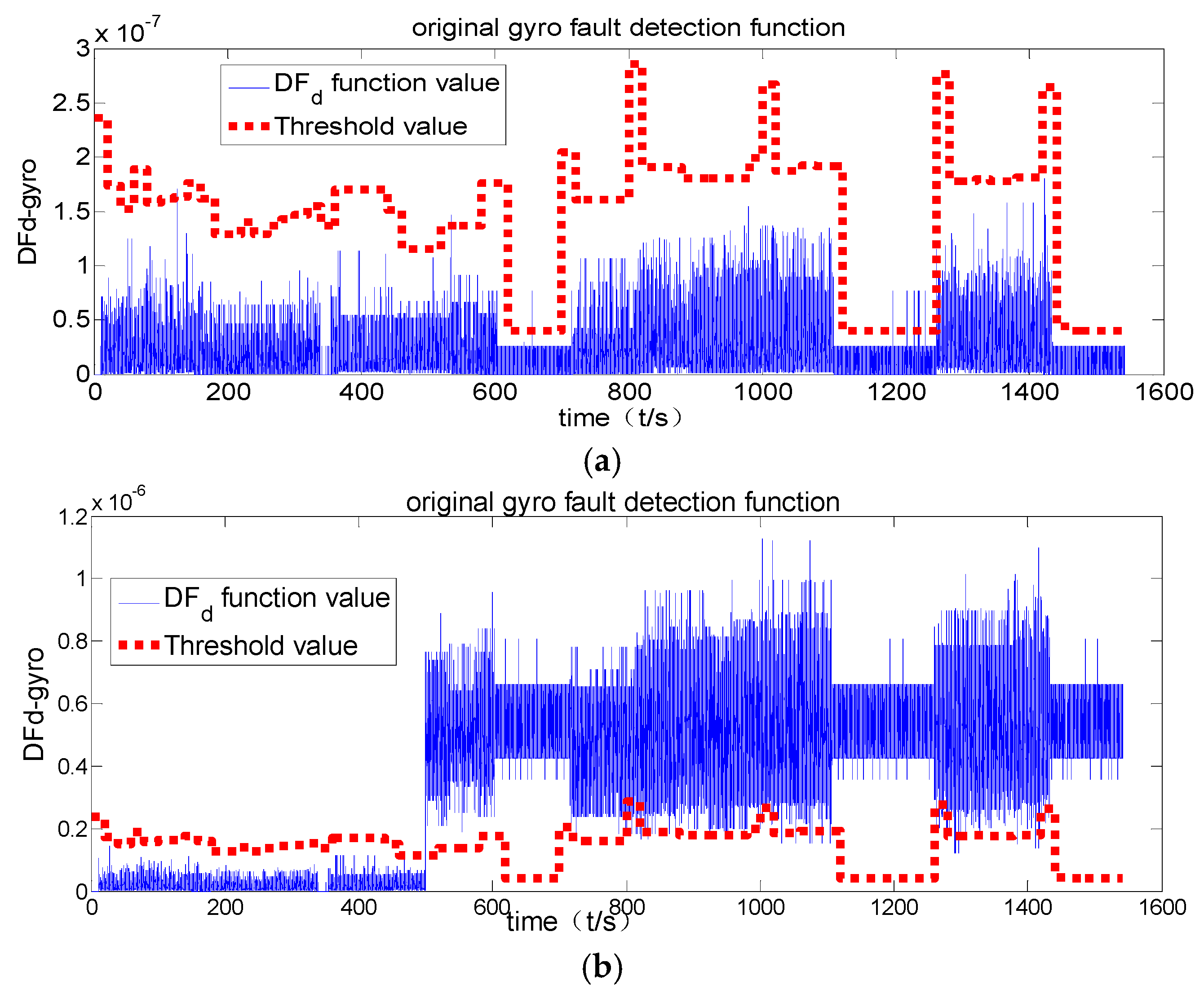
The quantization causes the problem that quantization errors make it difficult to detect fault correctly. The fault-tolerant air data inertial reference system (FT/ADIRS) developed by Honeywell is the most successful engineering product. The core component is a strapdown inertial reference system consisting of six GG1320 laser gyroscopes and six accelerometers (Hexad system) [23]. We take the hexad system as an example, which is shown in Figure 2. After experiments on quantization, we obtain the data on the inertial sensor, whose gyroscope bias is ${0.05}^{\circ }/\mathrm{h}$. We add faults of different amplitudes to the 1st gyroscope in 500 s. The simulation results are shown in Figure 3.

Observation matrix:

$$\mathit{H}=\left[\begin{array}{ccc}0.52573& 0& 0.85065\\ -0.52573& 0& 0.85065\\ 0.85065& 0.52573& 0\\ 0.85065& -0.52573& 0\\ 0& 0.85065& 0.52573\\ 0& 0.85065& -0.52573\end{array}\right]$$

(8)

As Figure 3a shows, the function value does not exceed the threshold value in the whole fault detection phase when the amplitude of fault is $5^{\circ }/\mathrm{h}$. However, when the amplitude of fault increases to ${100}^{\circ }/\mathrm{h}$, the fault can be detected with this method. At this time, the detection performance is essentially the same as the measurement not quantified. That is to say, the quantization error reduces the fault amplitude by about 20 times with the equivalent pulse. This paper develops the three-channel filter to solve the problems brought about by quantization.

2.2. The Three-Channel Filter for FDI

2.2.1. Fault Classification

Only when the amplitude of a gyroscope’s fault increases to ${100}^{\circ }/\mathrm{h}$ is the detection performance improved. There are three categories of fault according to its amplitude: hard fault, medium fault and soft fault [24]. The fault of a laser gyroscope has the following categories, as shown in

Table 1. Categories and amplitudes of fault.

Fault Type	Fault Magnitude
Hard fault	>$100°/\mathrm{h}$
Medium fault	$5°/\mathrm{h}$~$100°/\mathrm{h}$
Soft fault	≤$5°/\mathrm{h}$

(gyroscope bias: ${0.05}^{\circ }/\mathrm{h}$).

Hard fault has a comparatively large amplitude which primarily affects flight control performance. Medium fault has a medium amplitude which affects pilot display performance. Soft fault has a comparatively small amplitude which affects navigation performance.

2.2.2. The Three-Channel Filter

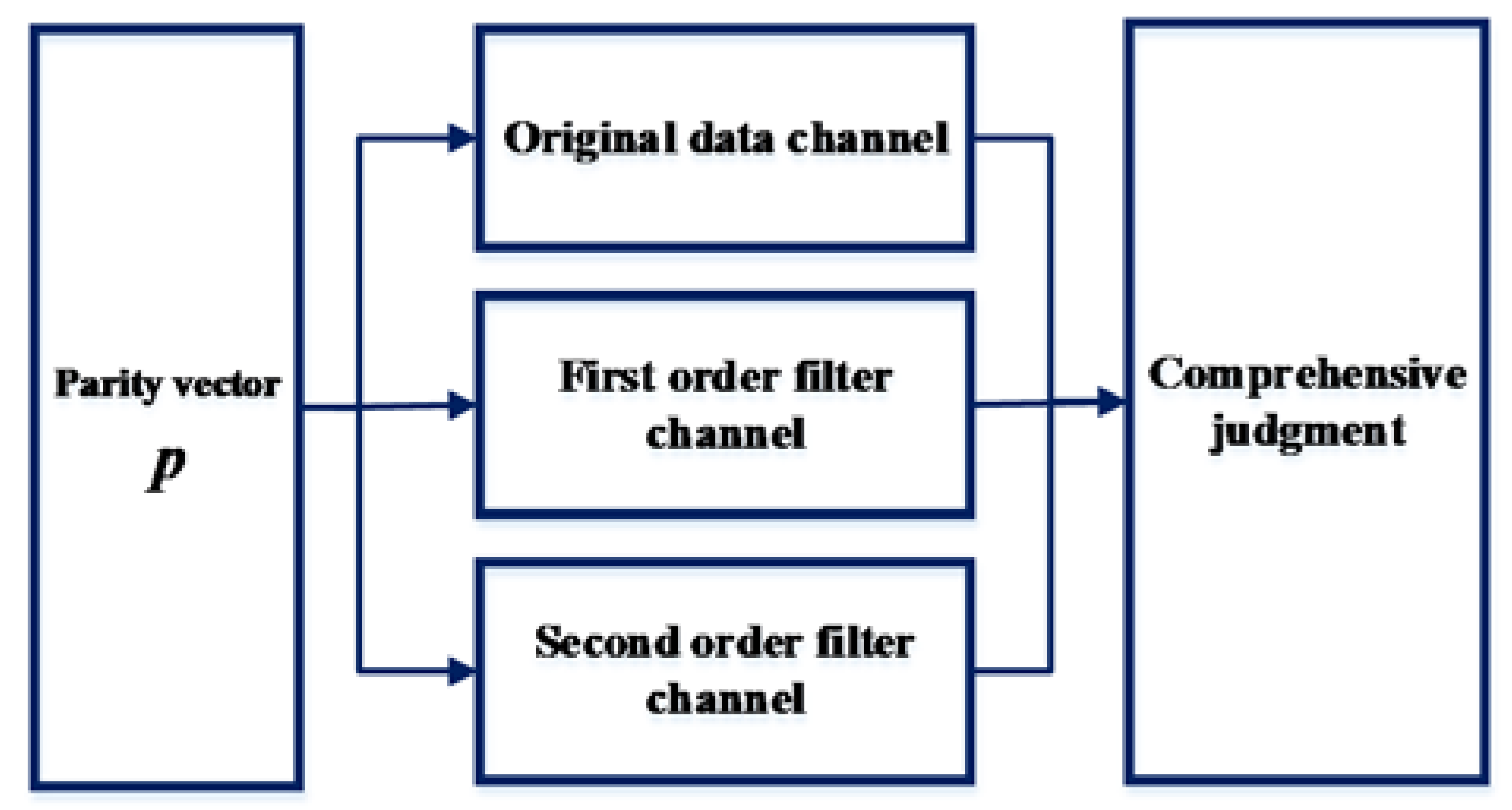
For a navigation system, faults of different amplitudes have different fault tolerance capabilities. The inertial sensor is integral and its errors accumulate over time. The hard fault must be detected immediately. The medium fault allows a fault tolerance system to have a short time delay. The soft fault has a slightly larger fault tolerance capability. Therefore, faults of different amplitudes should have different detection strategies. We use the three-channel filter to detect the three categories of fault in order to achieve better performance. The fault detection method based on the three-channel filter is shown in the following figure.

As is shown in Figure 4, each channel operates independently and does not affect each other. The procedures are classifying the faults according to their amplitude first, and then sending them to different fault detection channels. The original channel filter detects hard fault, the first-order channel detects medium fault, and the second-order channel detects soft faults.

2.2.3. The Filter Design

Based on the research and analysis of a low-pass filter, we put forward the constraint conditions that affect the fault detection performance: namely the cut-off frequency of the filter and its rising time. The cut-off frequency mainly affects false alarm rate and false isolation rate, while the rising time mainly decides the delay time of the FDI system. However, the cut-off frequency and the rise time are contradictory; therefore, we take the following compromise approach and theoretically analyze the parameters of the filter.

Original Channel

The large amplitude of hard fault does not allow the original channel filter to have time delay; therefore, this channel does not need preprocessing.

First-Order Channel Filter

First-order channel filter uses the first-order low-pass filter (time constant: $\mathrm{T}$)

$$G(s)=1/(\mathrm{T}s+1),$$

(9)

The rise time of the system represents rapidity.

$$T_r\approx 2.2\cdot \mathrm{T},$$

(10)

The low-pass filter can eliminate high-frequency noise so that only low-frequency signals can pass. Therefore, in order to achieve this goal, we make the cut-off frequency become small because when the signal frequency is smaller than the cut-off frequency, amplitude attenuation and phase attenuation are relatively small, and when the signal frequency exceeds the cut-off frequency, amplitude attenuation and phase attenuation both become quite large. Therefore, suppose there is an indication function:

$$y(\mathrm{T})=k_1{(2.2\mathrm{T})}^2+k_2(\frac{1}{\mathrm{T}}{)}^2,$$

(11)

where $k_1$ and $k_2$ represent the weights of rising time and cut-off frequency, respectively, which are decided by the performance of the FDI system. The reasonable choice of $k_1$ and $k_2$ can make the value $y(\mathrm{T})$ minimal. We obtain the following with the derivation of time constant $\mathrm{T}$ on both sides:

$$y^{\prime }(\mathrm{T})=9.68k_1\mathrm{T}-k_2\frac{2}{{\mathrm{T}}^3},$$

(12)

Let $y^{\prime }(\mathrm{T})=0$, and then we can obtain:

$$\mathrm{T}=0.6742\times \sqrt[4]{\alpha }\hspace{1em}\alpha =k_2/k_1,$$

(13)

where $\alpha$ expresses the ratio of cut-off frequency to rising time in the first- order channel filter. At the same time, it also indirectly indicates the ratio of false alarm rate to delay time for medium fault.

Second-Order Filter Channel

The transfer function of the critical damping system of the second-order channel filter can be defined as follows:

$$G(s)=\frac{1}{(\mathrm{T}s+1)(\mathrm{T}s+1)}=\frac{1}{{\mathrm{T}}^2{s}^2+2\mathrm{T}s+1},$$

(14)

The time constant of the second-order channel filter should be determined by the fault tolerance time of its soft fault. As we know, the smaller the time constant is, the faster the second-order channel filter responses. Thus, we should select a reasonable time constant and make the channel filter have a short response time and a low cut-off frequency. The weights of the performance indices of the response time and the cut-off frequency are $k_3$ and $k_4$, respectively. The rising time of the critical damping system is

$$T_r\approx 3.5\mathrm{T},$$

(15)

The cut-off frequency is inversely proportional to the time constant $\mathrm{T}$. The index function of the second-order channel filter is

$$y(\mathrm{T})=k_3{(3.5\mathrm{T})}^2+k_4(\frac{1}{\mathrm{T}}{)}^2,$$

(16)

The next step is the same as the first-order channel filter, and therefore we obtain

$$\mathrm{T}=0.5292\times \sqrt[4]{\beta }\hspace{1em}\beta =k_4/k_3,$$

(17)

According to the performance of the FDI method, we select $k_3$ and $k_4$ reasonably and obtain a proper time constant, where $\beta$ expresses the ratio of cut-off frequency to rising time in the second-order channel filter. At the same time, it indirectly indicates the ratio of false alarm rate to delay time for soft fault.

Brief Description

The first two parts present the calculation formula for analyzing the channel filter’s parameters, which are mainly affected by the weight of the ratio of cut-off frequency to rise time. Therefore, the channel filter’s parameters are chosen mainly through analyzing the changes in the ratio. Taking the second-order channel filter as example, the large ratio causes large parameters of the second-order channel filter; this means that the FDI system using the large parameters will have a lower false alarm rate and false isolation rate but a longer delay time. To detect soft fault, it is reasonable for the second-order channel filter to have large parameters.

3. Experiments Results and Analysis

3.1. Experiments Scheme

The experiments for step, ramp and square wave faults are carried out to evaluate the method performance. We add the faults to the 1st gyroscope in 500 s. The gyroscope error contains bias, scale factor error, installation error, random walk. The parameters used in experiments are shown in

Table 2. Parameters.

Parameter	Value ($1\mathit{\sigma }$)
Scale factor error	5 ppm
Installation error	$1^{″}$
Bias	$0.05{(}^{\circ }/\mathrm{h})$
Random walk	$0.01{(}^{\circ }/\sqrt{\mathrm{h}})$
Sample time	20 $\mathrm{ms}$

.

3.2. Experiments of Step Fault

3.2.1. The Comparison of Different Parameters

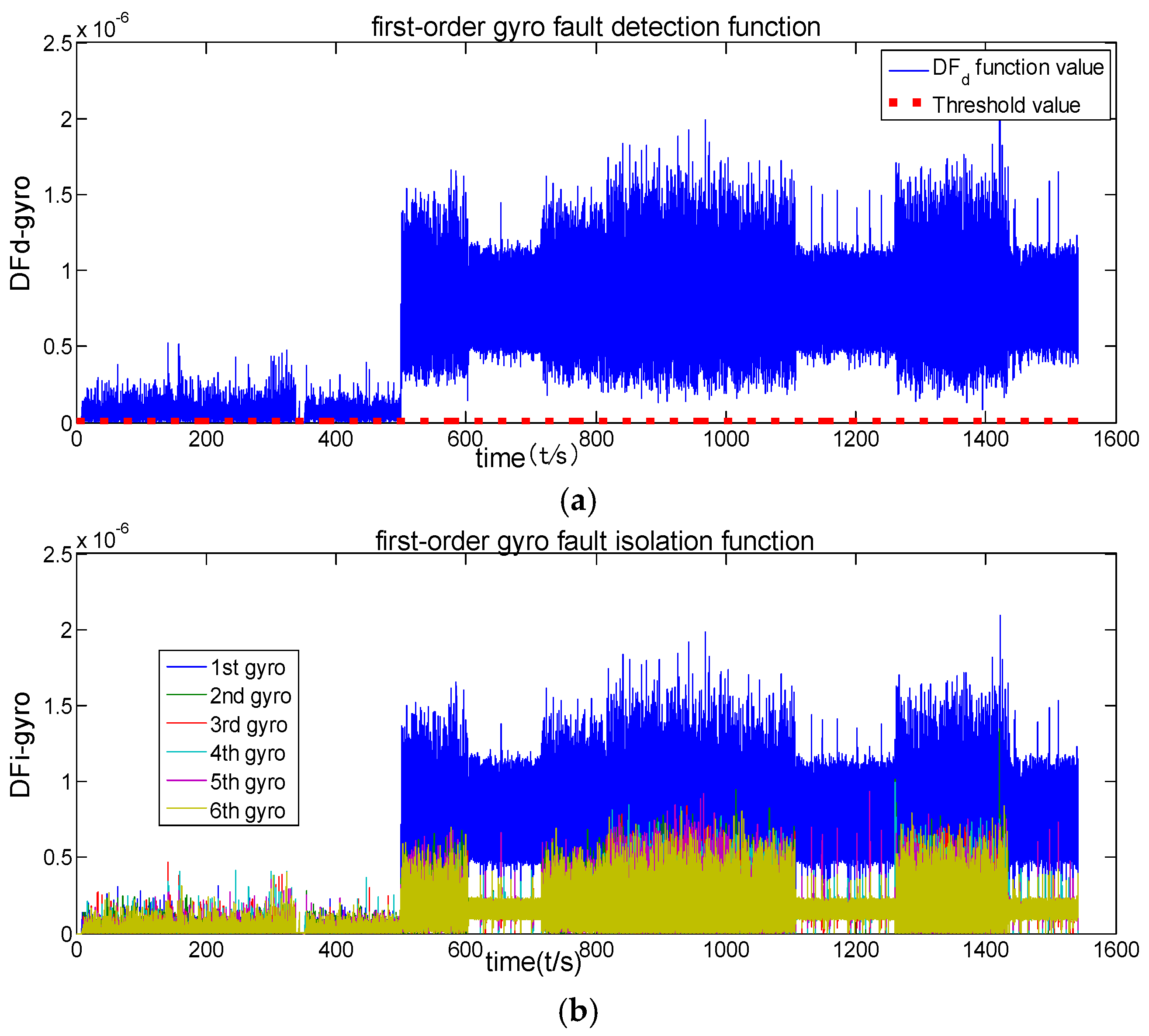
According to the analysis in Section 2, the parameters of the channel filter are not unique. Therefore, their comparison is made by using the step fault amplitudes of $5^{\circ }/\mathrm{h}$ and ${0.5}^{\circ }/\mathrm{h}$ in order to verify the correctness of the method proposed in this paper. Two fault amplitudes are added to the laser gyroscope. The parameters selected for the first-order and second-order channel filters are 0.434 and 3.85 (from Table 5) respectively.

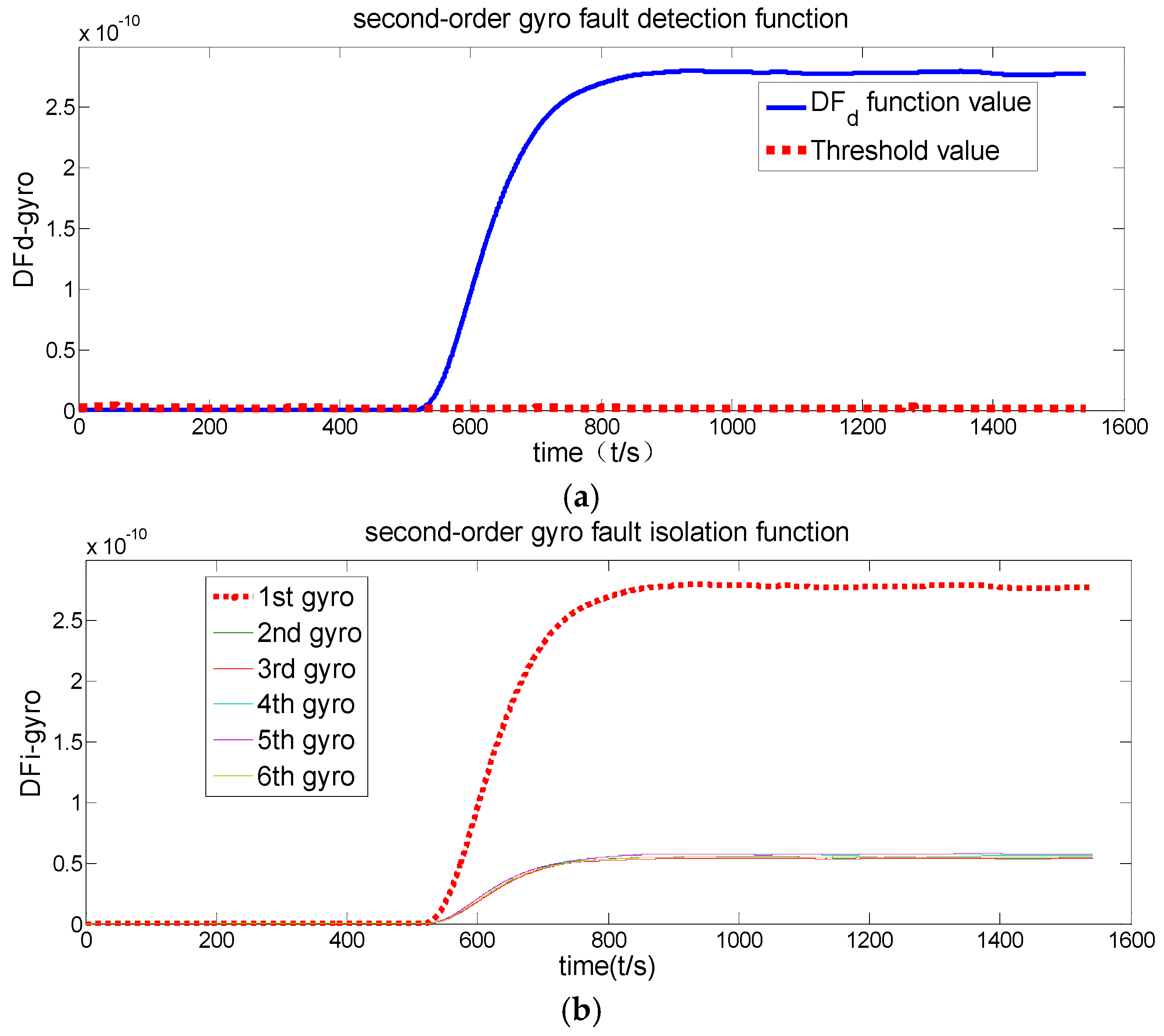
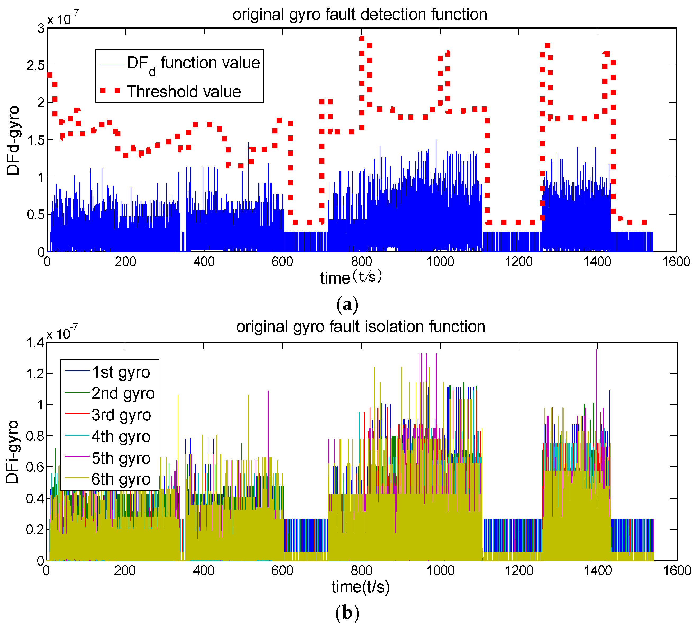
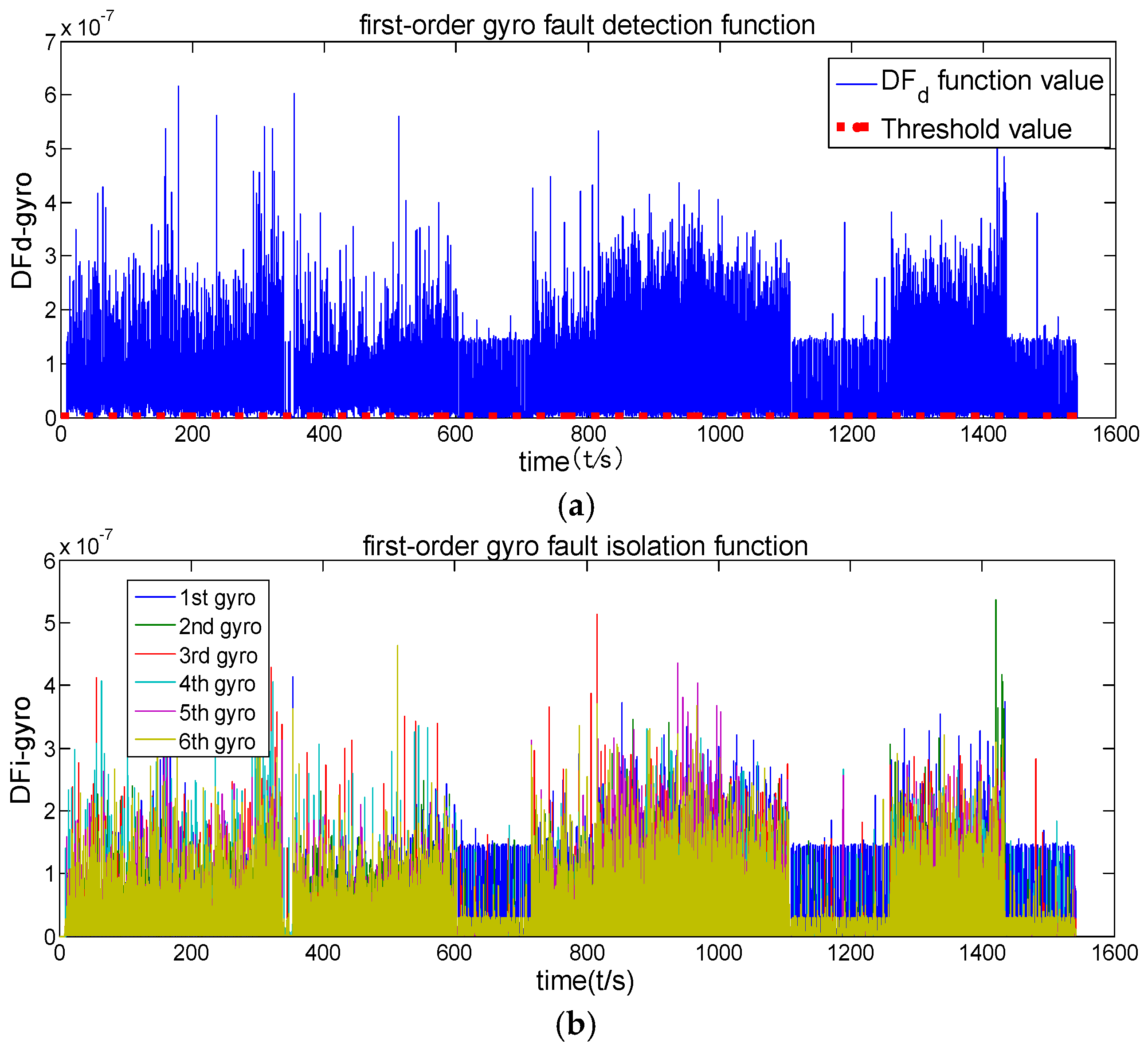
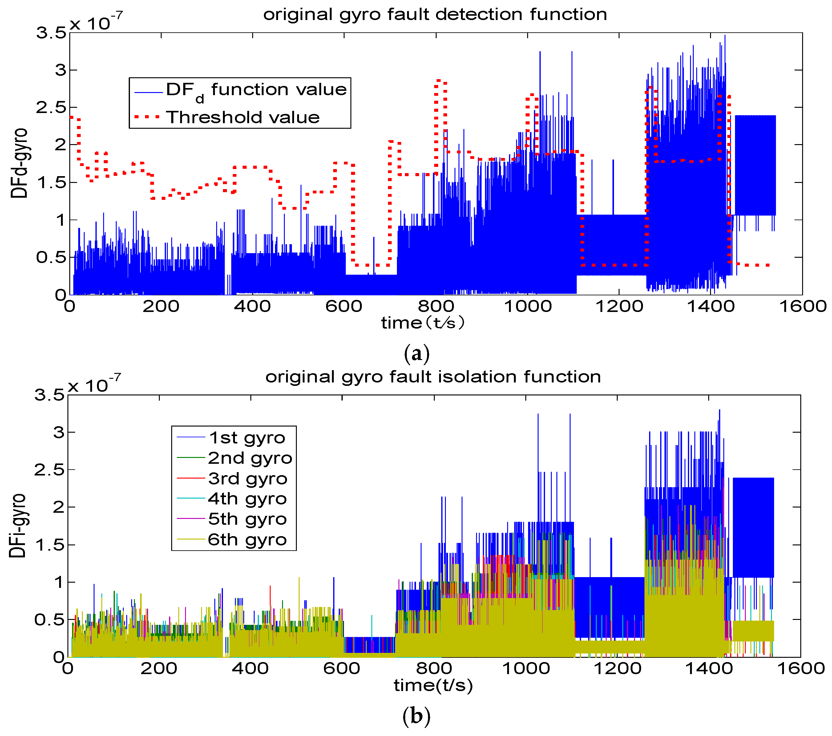
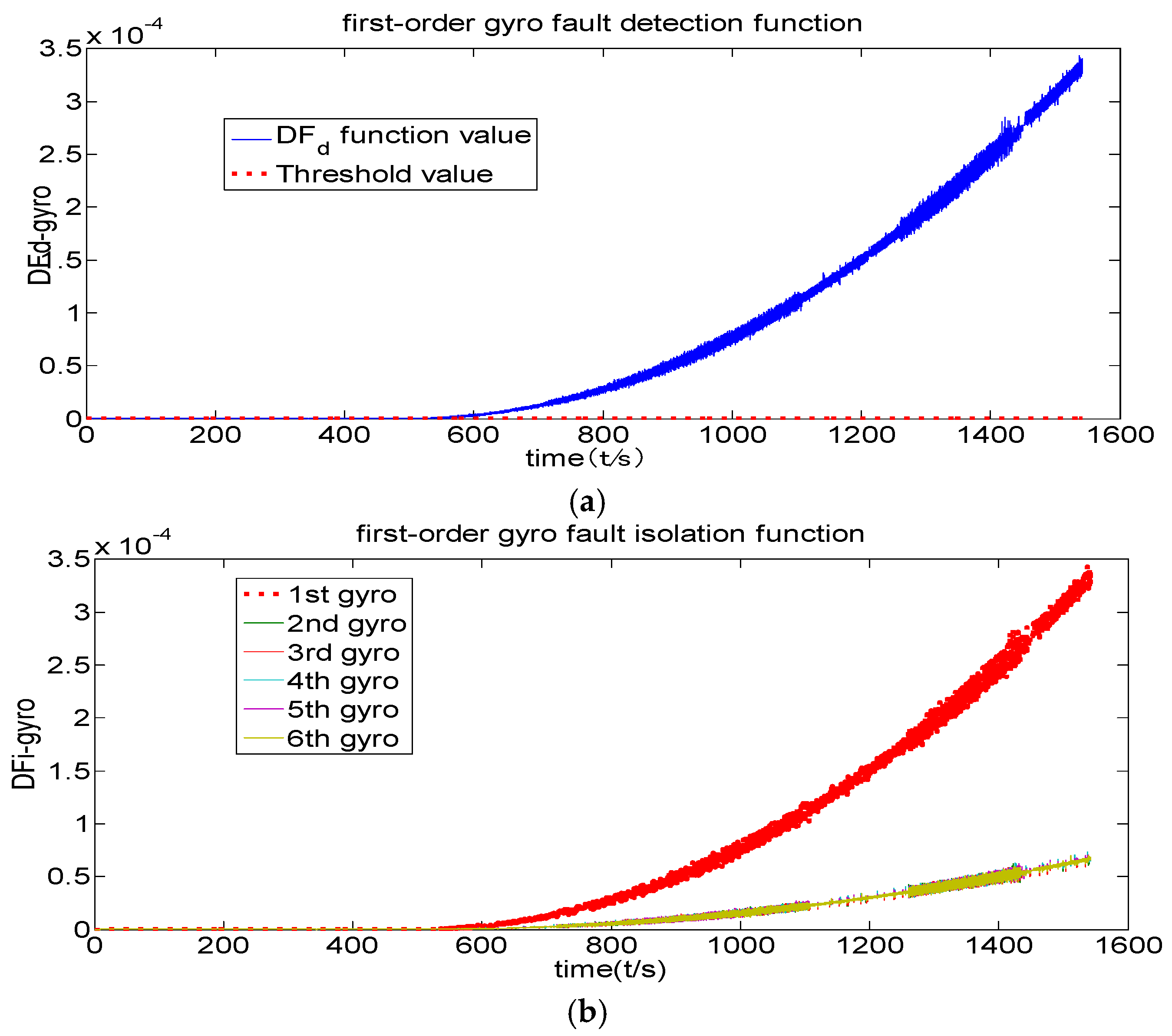
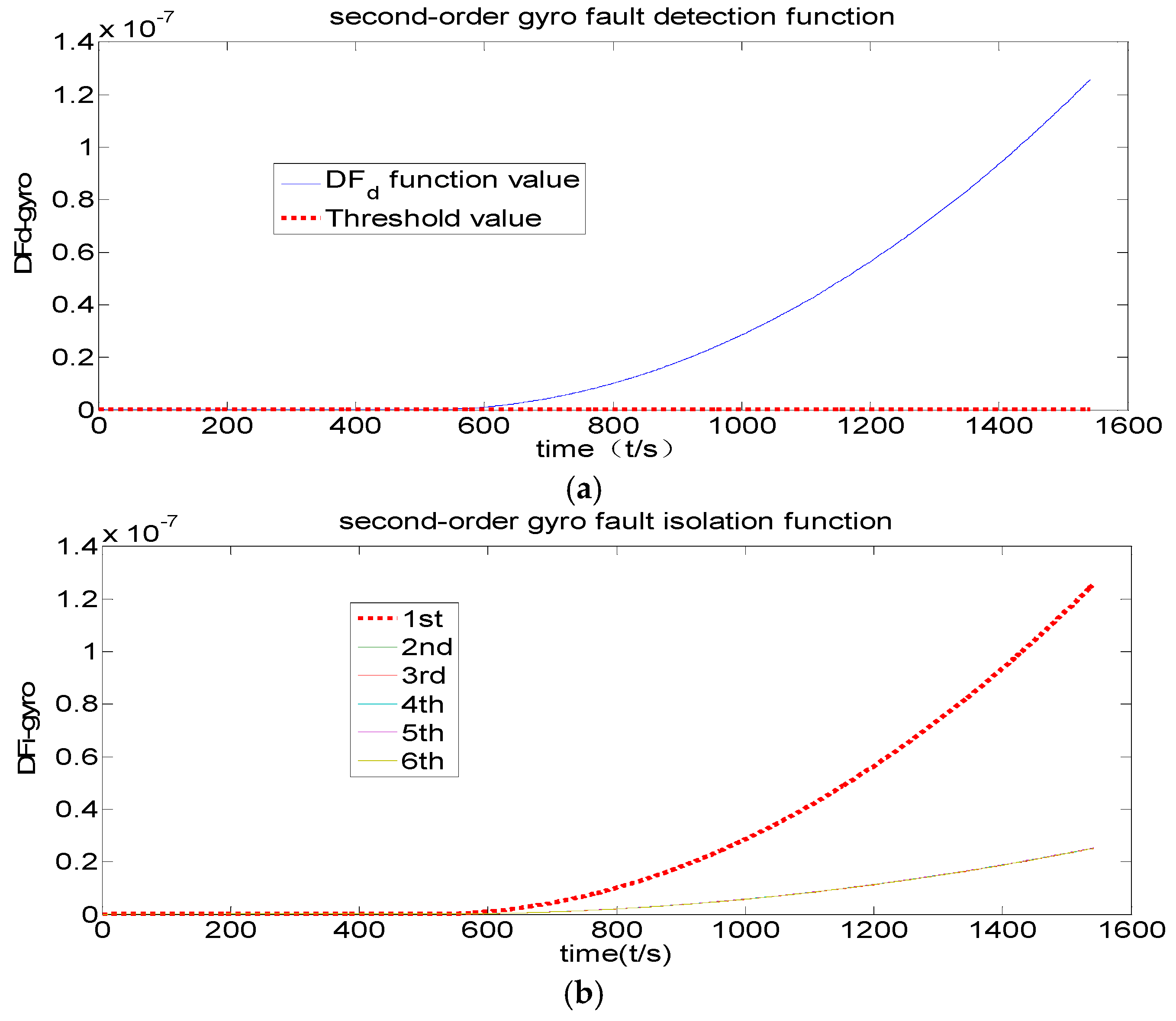
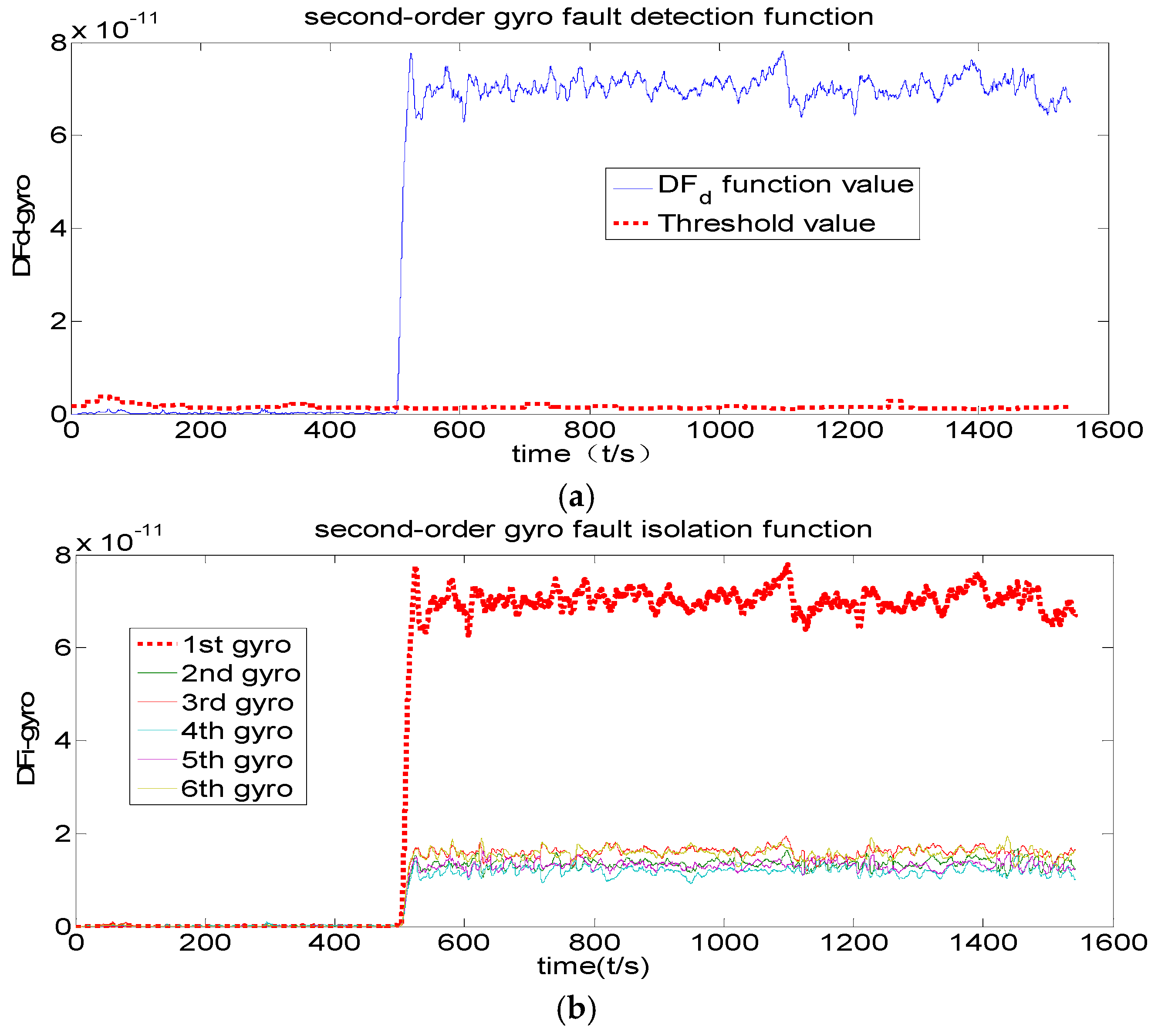
Figure 5 shows that the fault detection function of the original channel filter has never exceeded its threshold value, indicating that no fault has been detected. Figure 6 shows that the fault detection function exceeds the threshold value after 500 s, indicating that the first-order channel filter has detected a fault. Furthermore, its fault isolation function has been separated after 500 s, indicating that this channel filter is also able to isolate fault. Figure 6 also shows that fault is both detected and isolated correctly. The comparison of Figure 6 and Figure 7 indicates that the first-order channel filter’s detection delay time is relatively short but that its detection accuracy is not high (the curve is rougher). The second-order channel filter’s detection delay time is long but its detection accuracy (the curve is smoother) is high. Therefore, it is concluded that fault detection delay and detection accuracy are contradictory.

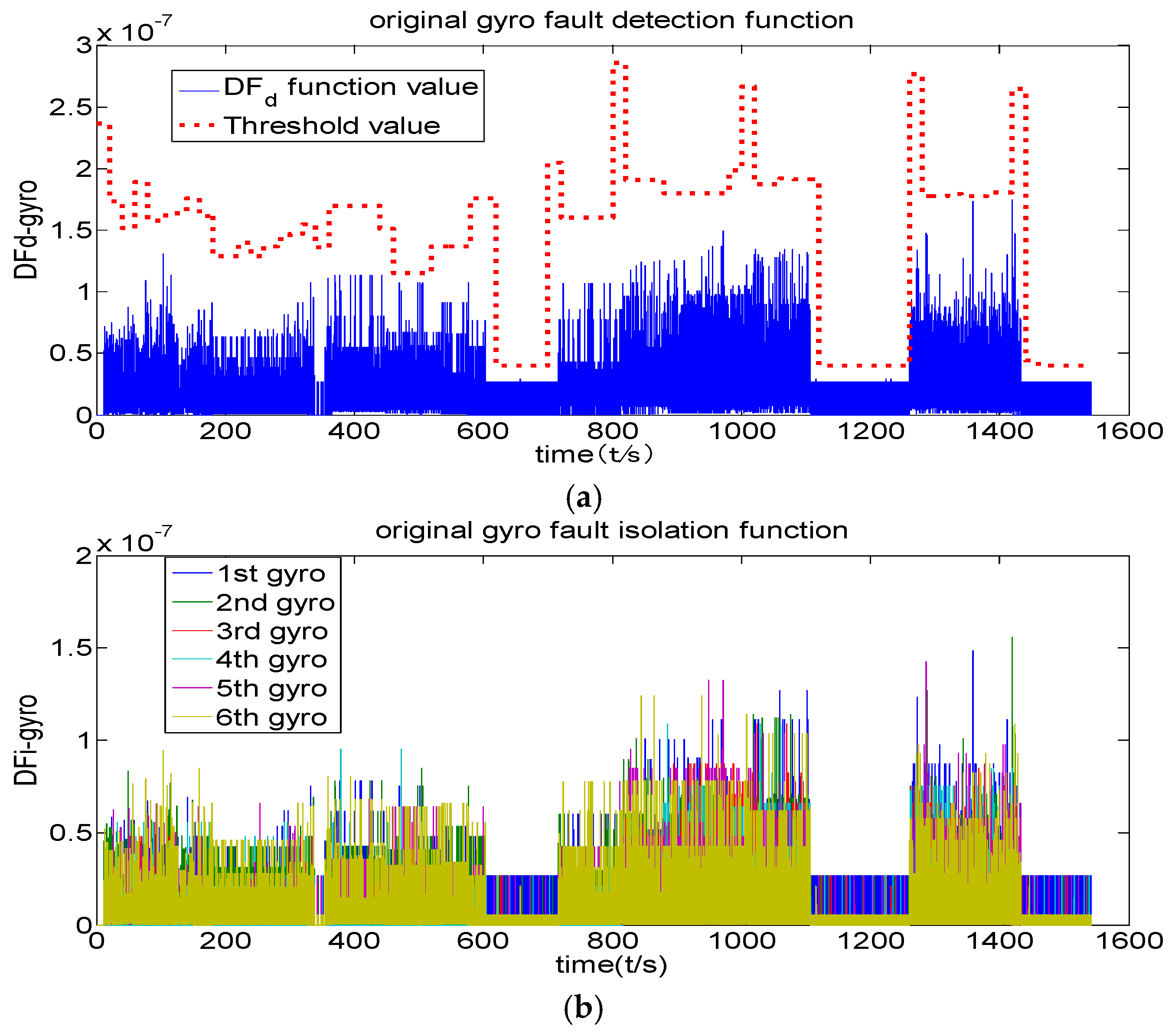
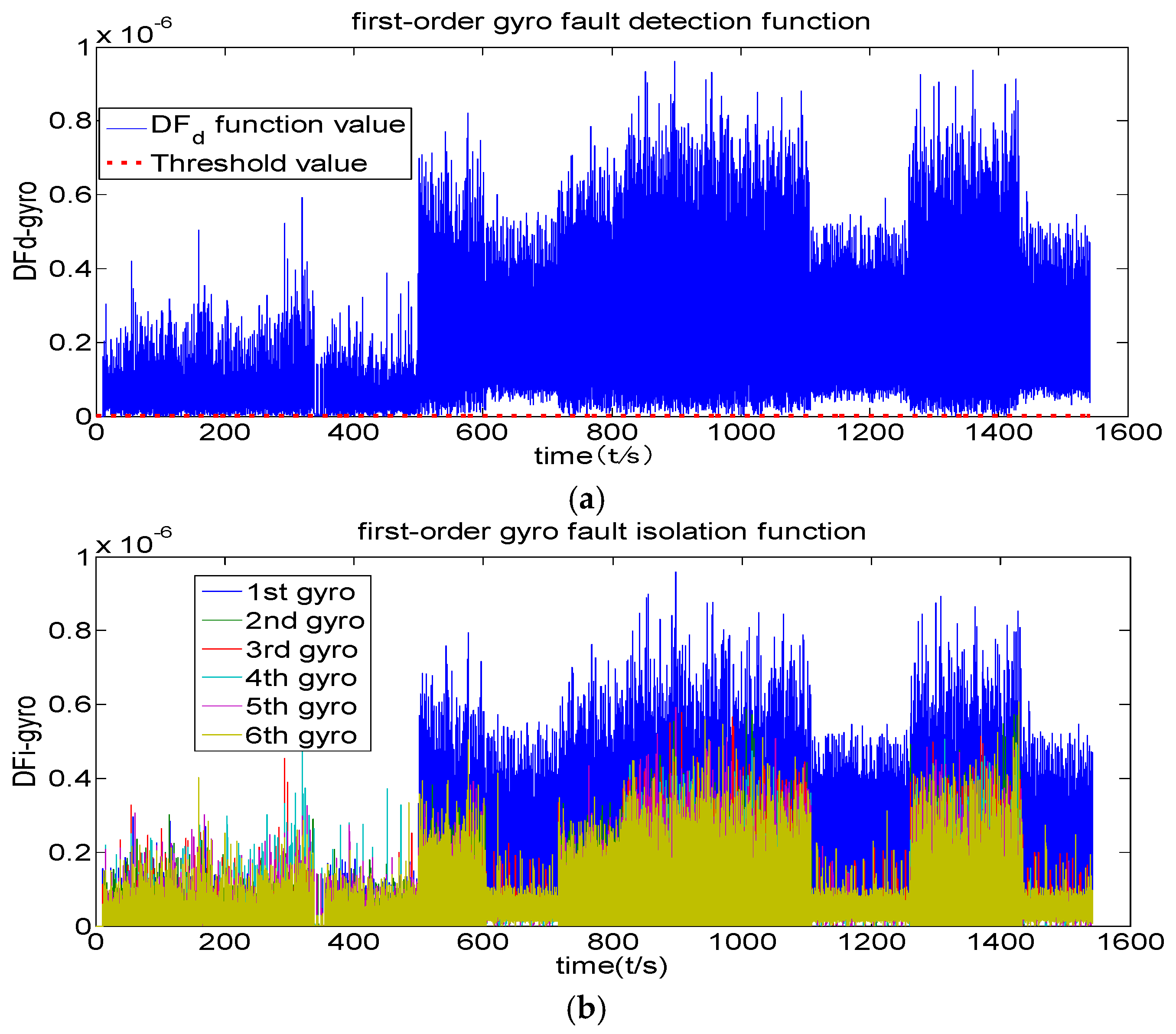
Figure 8, Figure 9 and Figure 10 show that the original channel filter and the first-order channel filter cannot detect a fault that has such a small amplitude. Figure 10 show that the fault detection function has exceeded the threshold value before 500 s, indicating that it has detected a fault.

Figure 5, Figure 6, Figure 7, Figure 8, Figure 9 and Figure 10, using the same sets of parameters of the channel filters, show that the first-order channel filter and the second-order channel filter can detect and isolate the fault that has a large amplitude. But the original channel filter and the first-order channel filter cannot detect the fault that has a small amplitude; only the second-order channel filter can.

3.2.2. The Monte Carlo Simulation

The first-order channel filter and the second-order channel filter use the same principles for parameter selection. Take the second-order channel filter as an example. The parameters of time constant, fault magnitude and sample time are considered in the Monte Carlo analysis.

With the different parameters (based on the ratio of cut-off frequency to rising time) of the second-order channel filter, its false alarm rate, false isolation rate and positive detection rate are calculated as 1000 times the Monte Carlo simulation. The statistical results are shown in

Table 3. The relationship between time constant and the effect on detecting faults (step fault $5^{\circ }/\mathrm{h}$ ).

Time Constant	3	3.85	5	8	10	20
False alarm rate	0.060	0.043	0.000	0.000	0.000	0.000
False isolation rate	0.277	0.050	0.060	0.040	0.020	0.000
PCD1	0.020	0.000	0.000	0.000	0.000	0.000
PCD2	0.880	0.760	0.680	0.100	0.000	0.000
PCD3	0.040	0.180	0.320	0.900	1.000	1.000
PCD4	0.000	0.000	0.000	0.000	0.000	0.000

(typical fault). In this table, the false alarm rate is defined as the probability of failure alarm without fault injection; the false isolation rate is defined as the probability of correctly detecting fault but not isolating it correctly. Their formulas are as follows. PCD 1 refers to the probability that a fault is detected within 1 s. PCD 2 refers to the probability that a fault is detected within 1 to 10 s. PCD 3 refers to the probability that a fault is detected within 10 to 100 s. PCD 4 the probability that a fault is detected within more than 100 s.

Table 3 helps draw the conclusion that with the increase of the parameters of the second-order channel filter, its false alarm rate and false isolation rate decreases, whereas the channel filter cannot detect any fault in a short time. Hence, we design and select the appropriate time constant according to actual conditions of RIMU.

When the parameter of the second-order channel filter is 3.85, we conduct the Monte Carlo simulations 1000 times to verify the detection effect of the same parameter on detecting the fault of different amplitudes.

Table 4. Calculation results of Monte Carlo simulations.

Fault Magnitude (${}^{\circ }/\mathbf{h}$)	5	0.5	0.4	0.3	0.2	0.1
False alarm rate	0.000	0.010	0.030	0.130	0.500	0.860
False isolation rate	0.030	0.626	0.773	0.724	0.740	0.786
PCD1	0.010	0.000	0.000	0.000	0.000	0.000
PCD2	0.960	0.690	0.260	0.090	0.010	0.000
PCD3	0.000	0.300	0.700	0.690	0.320	0.050
PCD4	0.000	0.000	0.010	0.090	0.170	0.090

shows that the same parameter of the second-order channel filter has different FDI effects on the faults of different amplitudes. The fault of a smaller amplitude leads to a worse FDI effect. In other words, to detect or isolate the fault of smaller amplitude, the FDI method may need a larger parameter.

Table 5. Parameters recommended for fault detection and isolation (FDI) with the typical fault in different sampling times.

Sample Time (s)	First Order Filter	Second Order Filter
0.020	0.434	3.850
0.040	0.600	5.000
0.060	0.650	6.000
0.200	5.000	15.000
0.400	8.000	20.000
1.000	10.000	30.000

recommends the parameters of the channel filters to detect or isolate a typical fault in different sampling time (the Monte Carlo simulation performed 1000 times; the step fault is $5^{\circ }/\mathrm{h}$; the false alarm rate and false isolation rate are 0.05 respectively).

3.3. Experiments of Ramp and Square Wave Faults

3.3.1. Ramp Fault

The ramp fault is 0.1 degree per hour. The FDI results are shown in Figure 11, Figure 12 and Figure 13. The parameters of the first-order and second-order filters are 0.434 and 3.85 respectively.

It is found that the ramp fault detection function of the original channel filter has never exceeded its threshold value in Figure 11, indicating that no fault has been detected. The Figure 12 shows that the fault detection function exceeds the threshold nearing 600 s, indicating that the first-order channel filter has detected a fault. However, its fault isolation function has been separated, nearing 600 s. Furthermore, Figure 13 shows that the fault detection function exceeds the threshold, also nearing 600 s, indicating that the second-order channel filter has detected a fault. Its fault isolation function has been separated nearing 600 s and the curve is smoother.

Similarly, we take the second-order channel filter as an example (the Monte Carlo simulation 1000 times). The statistical results are shown in the following

Table 6. The relationship between time constant and the effect on detecting faults (ramp fault).

Time Constant	3	3.85	5	8	10	20
False alarm rate	0.006	0.000	0.000	0.000	0.000	0.000
False isolation rate	0.702	0.720	0.600	0.560	0.540	0.240
PCD1	0.000	0.000	0.000	0.000	0.000	0.000
PCD2	0.940	1.000	0.860	0.100	0.020	0.000
PCD3	0.000	0.000	0.140	0.900	1.980	1.000
PCD4	0.000	0.000	0.000	0.000	0.000	0.000

.

3.3.2. Square Wave Fault

The amplitudes of square wave fault is $5^{\circ }/\mathrm{h}$, and the frequency is 5 Hz. The FDI results are shown in Figure 14, Figure 15 and Figure 16.

It is found that the fault detection function of the original channel filter has never exceeded its threshold value in Figure 14, indicating that no fault has been detected. Figure 15 and Figure 16 show that the fault detection function exceeds the threshold in 500 s, indicating that the first-order channel filter and the second-order channel filter have detected the fault.

Take the second-order channel filter as an example (the Monte Carlo simulation 1000 times). The statistical results are shown in the following

Table 7. The relationship between time constant and the effect on detecting faults (square wave fault).

Time Constant	3	3.85	5	8	10	20
False alarm rate	0.420	0.140	0.080	0.000	0.000	0.000
False isolation rate	0.448	0.442	0.130	0.160	0.080	0.122
PCD1	0.580	0.780	0.340	0.000	0.000	0.000
PCD2	0.000	0.080	0.580	1.000	1.000	0.440
PCD3	0.000	0.000	0.000	0.000	0.000	0.560
PCD4	0.000	0.000	0.000	0.000	0.000	0.000

.

4. Conclusions

This paper develops the three-channel filters to solve the problem that the conventional parity space approach cannot detect soft fault correctly after quantization. It proposes the constraint conditions of the filter design and implements them theoretically at a deep level, using the parity space approach. The proposed theory can provide a theoretical reference to improve the performance of the FDI system.

(1) Regarding the step fault, the Monte Carlo simulation results confirm that with the increases of time constant, the false alarm rate and the false isolation rate are both reduced but have a longer time delay. Therefore, when the fault amplitude is smaller, the FDI method needs a longer time for fault tolerance and we can choose a bigger parameter for the second-order channel filter according to the application environment.

(2) The relationship between time constant and the effect on detecting step fault is also studied in this paper using enumeration. Additionally, the parameters for detecting or isolating the typical step fault in different sampling times are recommended.

(3) The extended experiments have shown that the method could also detect and isolate the ramp and square wave faults. The time constant of the filters should be prolonged to achieve a low false alarm rate and low false isolation rate. Furthermore, the time constants of the ramp fault and the square wave fault require further investigation.

References

- Steven, R.H.; Paul, M.; Eliezer, G.; John, D. In-Flight parity vector compensation for FDI. IEEE Trans. Aerosp. Electron. Syst. 1983, 19, 668–676. [Google Scholar] [CrossRef]
- Richard, A.; Mckern, H.M. Redundancy management of inertial systems. In Proceedings of the AIAA Guidance and Control Conference, Key Biscayne, FL, USA, 20–22 August 1973; pp. 73–852. [Google Scholar]
- Kevin, C.D.; Eliezer, G.; James, V.H. Generalized Likelihood Test for FDI in Redundant Sensor Configurations. J. Guid. Control Dyn. 1979, 2, 9–17. [Google Scholar] [CrossRef]
- Paul, F.M. Fault diagnosis in dynamic systems using analytical and knowledge based redundancy-survey and some new results. Automatica 1990, 26, 459–474. [Google Scholar] [CrossRef]
- Medvedev, A. Disturbance attenuation enhancement in continuous parity space methods. In Proceedings of the 1997 European Control Conference (ECC), Brussels, Belgium, 1–4 July 1997; pp. 641–647. [Google Scholar]
- Hong, J.; Hong, Y.Z. Failure detection using optimal parity vector sensitive to special sensor failure. In Proceedings of the 1996 IEEE/SICE/RSJ International Conference on Multisensor Fusion and Integration for Intelligent Systems, Washington, DC, USA, 8–11 December 1996; pp. 55–61. [Google Scholar] [CrossRef]
- Hong, J.; Hong, Y.Z. Optimal Parity Vector Sensitive to Designated Sensor Fault. IEEE Trans. Aerosp. Electron. Syst. 1999, 35, 1122–1128. [Google Scholar] [CrossRef]
- Duk, S.S.; Cheol, K.Y. Geometric FDI based on SVD for Redundant Inertial Sensor Systems. In Proceedings of the 5th Asian Control Conference, Melbourne, Australia, 20–23 July 2004; pp. 1094–1100. [Google Scholar]
- Kwang, H.K.; Jang, G.L. Extension of Parity Space Approach for Two-Fault Detection and Isolation. In Proceedings of the AIAA Guidance, Navigation, and Control Conference and Exhibit, San Francisco, CA, USA, 15–18 August 2005. [Google Scholar] [CrossRef]
- Lee, W.H.; Kwang, H.K.; Park, C.G.; Jang, G.L. Two-Faults Detection and Isolation Using Extended Parity Space Approach. J. Electr. Eng. Technol. 2012, 7, 411–419. [Google Scholar] [CrossRef]
- Lee, W.H.; Park, C.G. A fault detection method of redundant IMU using modified principal component analysis. Int. J. Aeronaut. Space 2012, 13, 398–404. [Google Scholar] [CrossRef]
- Seung, K.K.; Youdan, K.; Chan, G.P.; Insung, J. Hybrid fault detection and isolation techniques for aircraft inertial measurement sensors. In Proceedings of the AIAA Guidance, Navigation, and Control Conference and Exhibit, Providence, Rhode Island, 16–19 August 2004; Volume 7, pp. 73–84. [Google Scholar] [CrossRef]
- Élcio, J.O.; Ijar, M.F.; Helio, K.K. Fault detection and isolation in inertial measurement units based on χ2-cusum and wavelet packet. Math. Probl. Eng. 2013, 1–10. [Google Scholar] [CrossRef]
- Ling, X.Z.; Ming, C.; Cui, P.L. Optimal parity vector method and generalized likelihood method for fault diagnosis of redundant sensors Equivalent test method. J. Northwest. Polytech. Univ. 2005, 23, 266–270. [Google Scholar] [CrossRef]
- Wen, X.F.; Tong, Z.; Zi, J.R. A new decoupling matrix construction method for fault detection and isolation of a redundant strapdown inertial measurement unit. Trans. Jpn. Soc. Aeronaut. Space Sci. 2017, 60, 60–63. [Google Scholar] [CrossRef]
- Yi, N.W.; Zi, J.R.; Kai, K.D.; Kai, C.; Jie, Y. A study on fault diagnosis of redundant SINS with pulse output. In Proceedings of the 2nd International Conference on Advances in Mechanical Engineering and Industrial Informatics (AIMEII 2016), Hangzhou, China, 10–13 May 2016; pp. 1096–1100. [Google Scholar] [CrossRef]
- Dhanup, S.P.; Rajasekar, N. A comprehensive review on protection challenges and fault diagnosis in PV systems. Renew. Sustain. Energy Rev. 2018, 91, 18–40. [Google Scholar] [CrossRef]
- Mehdi, H.; Farzad, R.S. Fault-tolerant supervisory controller for a hybrid AC/DC micro-grid. IEEE Trans. Smart Grid 2016, 1–15. [Google Scholar] [CrossRef]
- Mehdi, H.; Farzad, R.S. Determination of Maximum Solar Power under Shading and Converter Faults—A Prerequisite for Failure-Tolerant Power Management Systems. Simul. Model. Pract. Theory 2016, 62, 14–30. [Google Scholar] [CrossRef]
- Vahid, P.; Farzad, R.S.; Babak, N.A. Data driven sensor and actuator fault detection and isolation in wind turbine using classifier fusion. Renew. Energy 2018, 116, 99–106. [Google Scholar] [CrossRef]
- Mehdi, H.; Farzad, R.S. Analysis and detection of a wind system failure in a micro-grid. J. Renew. Sustain. Energy 2016, 8, 043302. [Google Scholar] [CrossRef]
- Potter, J.E.; Suman, M.C. Thresholdless Redundancy Management with Arrays of Skewed Instruments. Integr. Electron. Flight Control Syst. 1977, 15, 15–25. [Google Scholar]
- Charles, M. The technological evolution of inertial reference systems. In Proceedings of the 1996 IEEE Position Location and Navigation Symposium, Atlanta, GA, USA, 22–25 April 1996; pp. 336–343. [Google Scholar] [CrossRef]
- Motyka, P.; Landey, M.; Mckern, R. Failure Detection and Isolation Analysis of a Redundant Strapdown Inertial Measurement Unit; NASA: Washington, DC, USA, 1981; p. 15933.
Figure 1.
The quantization process.
Figure 2.
The hexad system configuration ().
Figure 3.
Fault detection results. (a) Step fault ; (b) Step fault .
Figure 4.
The fault detection method based on the three-channel filter.
Figure 5.
Original channel filter (the fault amplitude is ). (a) Fault detection; (b) Fault isolation.
Figure 6.
First-order channel filter (the fault amplitude is ). (a) Fault detection; (b) Fault isolation.
Figure 7.
Second-order channel filter (the fault amplitude is ). (a) Fault detection; (b) Fault isolation.
Figure 8.
Figure 9.
Figure 10.
Figure 11.
Original channel filter. (a) Fault detection; (b) Fault isolation.
Figure 12.
First-order channel filter. (a) Fault detection; (b) Fault isolation.
Figure 13.
Second-order channel filter. (a) Fault detection; (b) Fault isolation.
Figure 14.
Figure 15.
Figure 16.