Detection and Quantification of Damage in Metallic Structures by Laser-Generated Ultrasonics

College of Mechanical Engineering &The State Key Lab of Fluid Power Transmission and Control, Zhejiang University, Hangzhou 320027, China
*
Author to whom correspondence should be addressed.
Appl. Sci. 2018, 8(5), 824; https://doi.org/10.3390/app8050824
Submission received: 23 April 2018
/
Revised: 16 May 2018
/
Accepted: 17 May 2018
/
Published: 20 May 2018
Abstract
:The appearance of damage on metallic structures is inevitable due to complex working environments. Non-destructive testing (NDT) of these structures is critical to the safe operation of the equipment. This paper presents a non-destructive damage detection, visualization, and quantification technique based on laser-generated ultrasonics. The undamaged and damaged metallic structures are irradiated with laser pulses to produce broadband input ultrasonic waves. Damage to the structures plays the role of a nonlinear radiation source of new frequencies. Usually these new frequencies are too weak to be detected directly. Here, the state space predictive model is proposed to address the problem. Based on the recorded responses in the time domain, the state space attractors are reconstructed. Damage to the structures is shown to change the properties of the attractors. A nonlinear damage detection feature called normalized nonlinear prediction error (NNPE) is extracted from the state space to identify the changes in the attractors—and hence the damage. Furthermore, the damage is visualized and quantified using the NNPE values extracted from the entire area by using a laser scanning technique. Experimental results validate that the proposed technique is capable of detecting, visualizing and quantifying artificial damage to aluminum alloy plates and actual fatigue cracks to a twin-screw compressor body.

1. Introduction
During the life cycle of a metallic structure, the appearance of damage is inevitable due to the structure’s complex working environments [1,2,3]. For example, the working environment of engine blades is very severe. These blades suffer from shock, friction and high temperatures as well as heating and cooling cycles. Therefore, it is very easy to produce cracks in the engine blades [1]. According to the statistics on predecessors, the failures in metallic structures caused by fatigue cracks account for more than 90% [4]. Each year, the breakdown and disorderly closedown of equipment caused by fatigue cracks cause owners to expend large amounts of time and money, and sometimes failures even threaten the operators’ safety and lives [5,6]. These safety and economic considerations have spurred research within the field of NDT of metallic structures in the past few years.
Among various structural damage detection techniques, such as infrared testing [7], eddy current testing [8,9], magnetic particle testing [10], and ultrasound testing [11,12], the ultrasound testing technique has been widely used due to its relatively high spatial resolution, portable operation, high performance ratio, and high effectiveness in damage detection. By recording the ultrasonic waves propagating through a structure, macroscopic damage such as cracks, inclusions, and notches can be detected by using this method [5]. Influenced by the linear interaction between propagating waves and damage, the ultrasonic waves experience reflection, diffraction, and mode conversion. By extracting metrics from the response waves, the damage can be defined. Notably, most damage detection techniques use linear metrics extracted from response waves to detect damage, namely, the damage is assumed only to affect the structure in a linear way. However, according to Worden’s study [12], damage evolution is a nonlinear process that initiates certain nonlinear properties in the structure. When dealing with nonlinear damage, linear ultrasonic waves may lose their effectiveness and reliability.
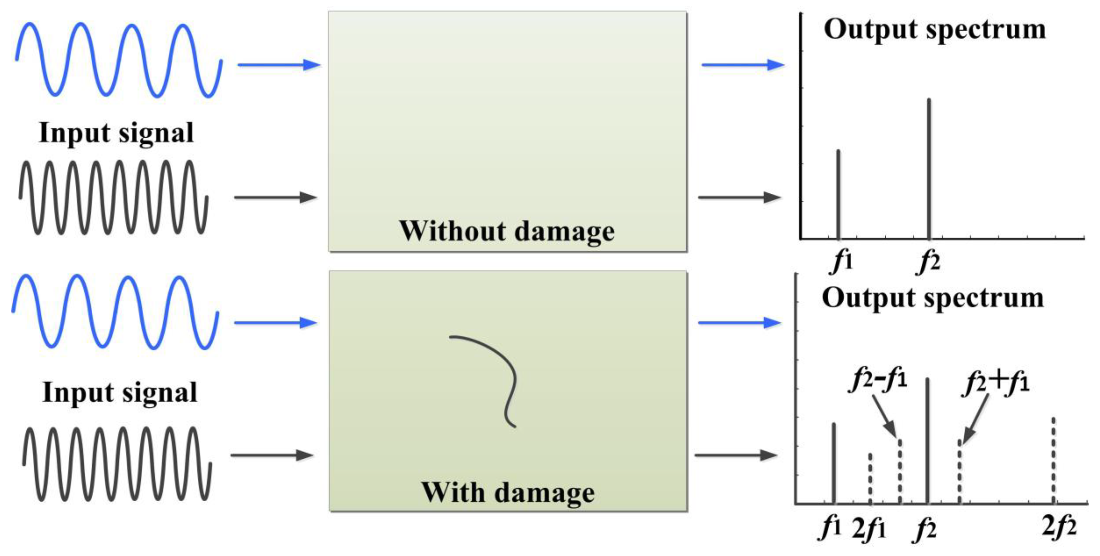
Recent studies have shown that nonlinear ultrasonic waves are usually more sensitive to small cracks than classical linear ones. In the nonlinear ultrasonic techniques, a fatigue crack plays the role of a nonlinear radiation source [13]. It will distort the original propagating ultrasonic waves and generate different waves with new frequency components as shown in Figure 1. This makes the new nonlinear component a damage-sensitive feature for damage detection. Duffour et al. [14] investigated the application of the nonlinear vibro-acoustic modulation technique for the assessment of fatigue cracks in steel beams and nickel-based alloy plates. In their experiments, the specimens were subjected to both a low ultrasound frequency and a low structural vibration frequency. The ratio of the average first sideband amplitude over the ultrasonics carrier was proposed as a nonlinear feature to assess the cracks. Jiao et al. [13] also investigated the application of the vibro-acoustic modulation technique for the detection of cracks in steel pipes. They delimited the Modulation Index as a crack-sensitive feature. The influence of the frequency and amplitude of vibration on the sideband amplitudes was experimentally investigated. Liu et al. [15] conducted nonlinear modulation measurement for non-destructive testing of the cracks in aluminum plates and scaled steel shafts. The nonlinear spectral coefficient was used to isolate the nonlinear modulation components from noisy environments and show a higher sensitivity to fatigue cracks than the traditional nonlinear coefficient. Hess et al. [16] investigated the application of the linear surface acoustic waves and the nonlinear surface acoustic waves in non-destructive testing of surface cracks. They demonstrated that the nonlinear surface acoustic waves could be more effective to crack detection. Gusev et al. [17] developed a theoretical model for crack imagination by the nonlinear frequency-mixing technique. Based on the model, the cracks in a glass plate were successfully detected and imaged [18]. They demonstrated that the sensitivity of this technique is 20 times higher than the linear photo-acoustic techniques.
In the research mentioned above, the nonlinear ultrasonic technique was demonstrated to be a good candidate for the detection of fatigue damage. However, this technique also has some shortcomings in that it is challenging to get the two most suitable independent original excitation frequencies in practice [19]. This is because the optimal choice of the excitation frequencies is also affected by the structure to be detected and the environmental condition [20]. Here we introduced the laser-generated ultrasonics technique [21] to solve this problem. Compared with traditional nonlinear techniques, only one laser pulse excitation is used to generate a broadband input signal rather than two different ultrasonic waves. So the optimal choice of the excitation frequencies is no longer a problem. But a new problem has reared up that is affected by the broadband nature of the input signal generated by the laser pulse. The new frequencies caused by the damage are submerged and cannot be detected directly. In this paper, we introduced the state space predictive model [22] to tackle this problem. The dynamic characteristics of the structure can be described by geometric figures in the state space and the damage is shown to change the properties of the geometric figure. By identifying the change in the geometric figure, the damage can be detected. Usually, the state space predictive model was applied to the vibrating structures for structural damage identification. In this paper, the model was applied to laser-generated ultrasonic signals for fatigue damage detection and quantification.
This paper is organized as follows: in Section 2, the fundamental issues about the generation and modulation of laser-generated ultrasonics and attractor-based analyses are provided. How damage can be detected and quantified by normalized nonlinear prediction error is also described in Section 2; in Section 3, a laser-generated ultrasonics detecting system is built to detect the damage; in Section 4 and Section 5, artificial damage to aluminum alloy plates and actual fatigue cracks in a twin-screw compressor body are detected and quantified by the proposed technique to validate the effectiveness of the technique. Finally, the results of this work are presented in Section 6.
2. Background
The fundamental issues of laser-generated ultrasonics and attractor-based analyses are briefly reviewed in this section. The framework for damage detection and quantification is provided. Transforming the dynamic properties of a structure into a geometric figure in the state space is shown to be especially useful for damage detection and quantification.
2.1. Generation and Modulation of Laser-Generated Ultrasonics
The ultrasonics technique has been used for damage detection for a long time, and the generation of ultrasonic waves by using laser pulses was developed in the 1960s [21]. When the surface of a material is illuminated by a laser pulse, the material absorbs a part of the laser energy, resulting in a rapid temperature rise in the local area. Elastic waves are generated due to the thermal expansion. Based on the power density of the irradiating pulse laser, there are two thermal models for the generation of ultrasonic waves, namely, ablation generation and thermo-elastic generation [23]. For the latter, the power density of the laser pulse is lower than the ablation threshold of the irradiated material, which indicates non-destructive wave generation. In this paper, thermo-elastic generation is considered.
After irradiation by a laser pulse, a broadband ultrasonics is generated. The ultrasonics is then used as an excitation signal to detect the damaged structure. When the wave is propagating in the structure, nonlinear wave modulation will occur because of the damage and new frequency components are generated as shown in Figure 2. Taking a closer look at Figure 2, the high-order nonlinear modulation signals are easily submerged by the original signal because of the broadband characteristic of the input signal, which means that traditional nonlinear damage detection technologies are unsuitable for this situation. State-space predictive models [22,24] are introduced to tackle this issue.
2.2. Reconstruction of the State-Space Attractor
Usually, a dynamic system can be described by a first-order differential equation:
where is a function of the variables x and t. Variable x represents the state variable and t represents time.
If we plot x1(t) against x2(t), the resulted space is called to be ‘state space’. If the solution of the equation is visualized as a trajectory in state space, for a given set of initial conditions, , the trajectories representing the dynamic properties of the system in the state space will trace out a unique path. After a certain period of disturbance, the path will gradually migrate towards an invariant geometric figure in state space. This geometric figure is called to be ‘attractor’ [22].This attractor in state space represents the steady state point of a dynamic system and exhibits sensitive dependence on the initial conditions of the system. This is the reason why the state space predictive model can be used for identifying the dynamic change (usually caused by damage) of a system [22,24,25,26]. Usually, an initial baseline attractor is reconstructed for an intact system and compared with the attractor reconstructed for a damaged one. Damage has been shown to change the geometry of the attractor. Hence, by identifying a change in the geometric properties, damage can be detected and even quantified. This is the basic damage detection principle of this paper.
In theory, all the vector variables of the system are needed to reconstruct the attractor. Unfortunately, it is difficult to obtain every vector variable in practice. Luckily, according to the embedding algorithm proposed by Takens [27], the unknown variables can be reconstructed by the measured ones. Assuming x(n) is the measured time series, the attractor X(n) can be expressed as follows:
where n is the discrete time index of the sampled value; m is the embedding dimension, it is the dimension of the reconstructed state space; T is the time delay, and all of the reconstructed vectors are simply time-delayed versions of the measured signal with a lag of T. The choice of parameters T and m influences the reconstruction result. In this study, the commonly acknowledged methods for the choice of the time delay T and embedding dimension m, namely, the average mutual information function (AMI) [28] and Cao’s function [29], are proposed to calculate the embedding parameters.
2.3. Feature Extraction
As indicated earlier, damage to a system is expected to alter the geometric portrait of the attractor in the state space. The difference between the undamaged and damaged attractors then becomes a good candidate feature for damage detection. Here, we introduce a certain metric called NNPE as the feature to identify the difference between the attractors.
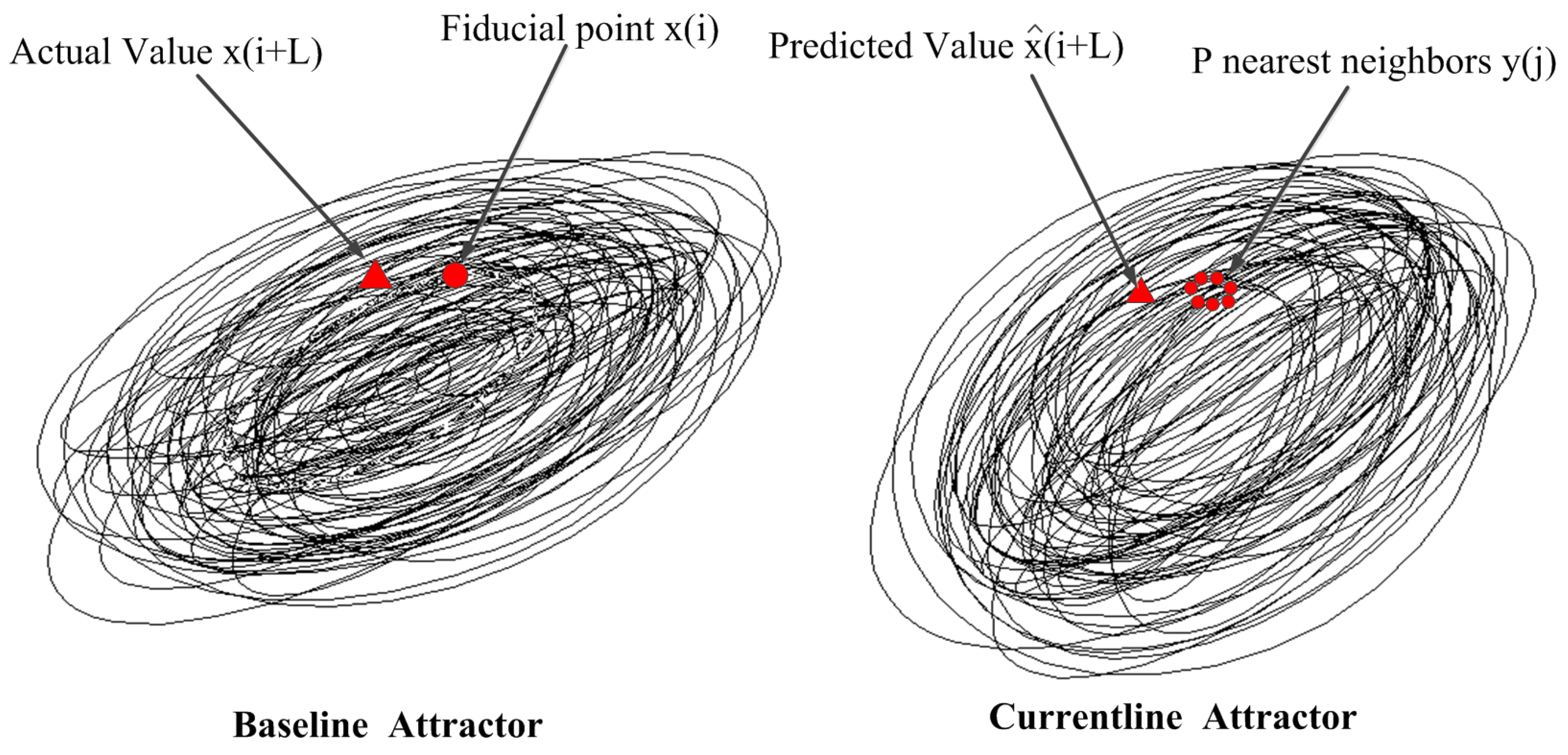
A schematic overview of feature NNPE extraction from the reconstructed state-space attractors is provided in Figure 3. First, P random points x(i) (i = 1,2,…,P) are selected from the baseline attractor reconstructed from the undamaged system. The selection of the value of P influences the feature extraction result. P is set to N/100 in this study based on Pecora’s work [30], where N is the number of recorded data. Next, Q points y(j) (j = 1,2,…,Q) closest to each point x(i) are selected from the current-line attractor reconstructed from the compared system, which may suffer from certain damage. When selecting the closest Q points in current-line attractor, the same P points x(i) (i = 1,2,…,P) will be used in the baseline attractor. For example, if point (1, 1) was selected as the random point in baseline attractor, then the point (1,1) will still be selected as the point in the current-line attractor. Even though in most cases, this point may not be contained on the trajectory in the current-line attractor. When the point x(i) is selected in the current-line, the closest Q points in the current-line attractor will be selected by the Euclidean distance of the specific point from the point x(i) in the state space. The Q points that have the shortest Euclidean distance from the point x(i) in current-line attractor will be selected as the closest Q points. Also, the choice of the value of Q should guarantee that the local dynamic properties of the attractor can be described clearly and that the feature extraction results will not be hidden by the noise. A proper choice is Q = N/1000 [31]. Meanwhile, to avoid the time correlation between x(i) and y(j), a Theiler Window with a step 2T is proposed when selecting the neighboring points. In this way, the minimum separation between x(i) and its closest neighbors in time will be at least 2T. After that, x(i) and y(j) will be evolved with L steps (L = 2 in this study) into the future. The prediction value of x(i) after L steps in time, , can be computed by
Once the prediction has been made, the prediction error can be computed by
where is the Euclidean norm. Finally, NNPEis proposed to capture the differences between the baseline and current-line attractors. NNPE is defined as [32]
where is the variance of the baseline signal. Obviously, this NNPE value is the quantity used for determining the differences between the baseline attractor and the current-line attractor caused by damage. The NNPE is selected as the damage-sensitive feature in this study.
2.4. Damage Detection and Quantification
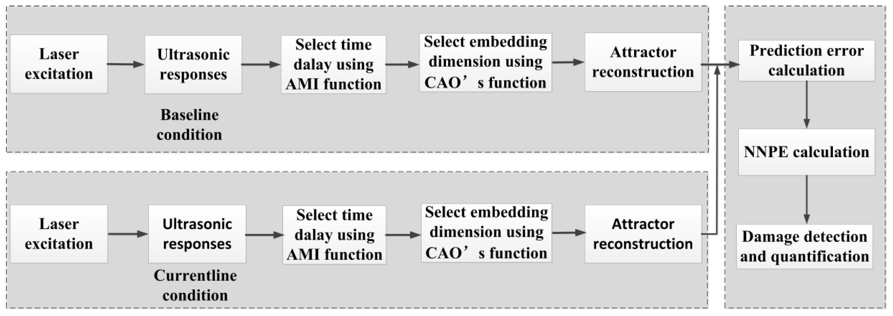
The laser scanning technique is introduced to visualize and quantify the damage. Any desired point on the structure surface can be irradiated by a laser pulse using a galvanometer, and the pitch between the two adjacent points is set to a constant. When a laser pulse is shot at a point, ultrasonic waves are generated because of the thermal expansion of the material. The ultrasonic waves propagating in the structure are then recorded by the transducer placed at a fixed point. The recorded ultrasonic responses from undamaged and damaged structures are used to calculate NNPE values for each excitation point to capture the differences between the baseline and current-line attractors. The most significant differences should occur at the damage location. Therefore, the damage can be detected by the calculated NNPE values. Notably, only a small area covering the damaged location in the damaged structure was scanned in this study to readily detect the damage because the damage location is not known in advance. Furthermore, the pitch between two adjacent points in the scanned area is determined before laser scanning, by counting the number of points that correspond to larger NNPE values in the visualization picture. The size of the damage can be quantified too.
A schematic diagram of the proposed technique is provided in Figure 4.
3. Experimental Setup and Testing Structures
3.1. Laser-Generated Ultrasonics Damage Detection System
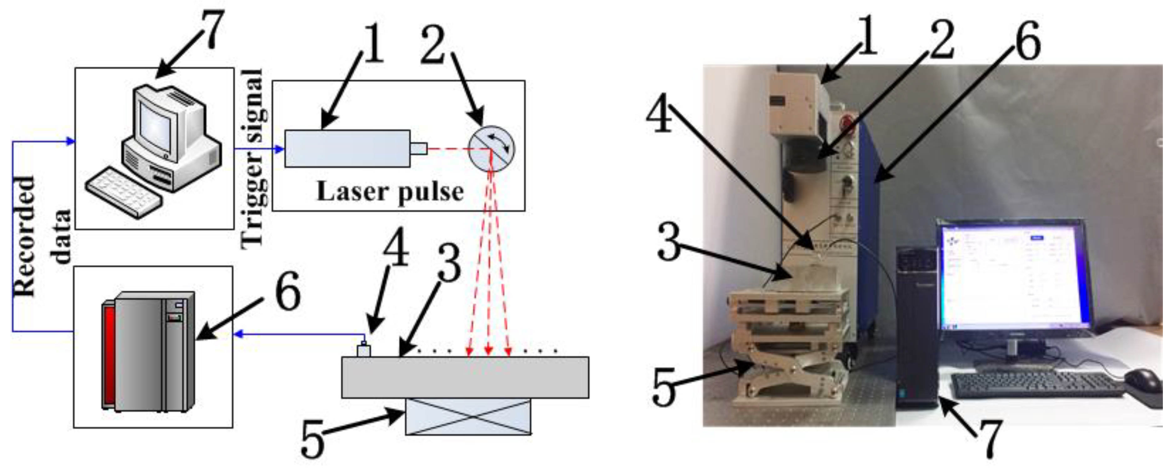
A laser-generated ultrasonics damage detection system was built in this study to verify the accuracy of the detection technique. A pulsed laser beam with a duration of 20 ns and at a repetition of 20 KHz is generated by a Q-switched Nd:YAG pulse laser. The wavelength of the pulse is 1064 nm. The laser pulse is slightly focused to a 0.3 mm diameter by a lens, and the maximum pulse energy density is controlled below 1 × 10⁷ W/cm2 to avoid ablating the material. Through the galvanometric scanner, the laser pulse can be shot at any desired place on the structure. The generated ultrasonic waves are recorded by a focused transducer mounted at a fixed point on the structure. The transducer used here is a high-frequency transducer product by Olympus (VB213 -RM) with a bandwidth frequency of 0–30.0 MHz, and the crystal diameter of the transducer is 6 mm. This transducer is used for receiving the surface acoustic waves generated by the laser pulse. Glycerin is used as the couplant to fix the transducer to the structure surface. Each dynamic response is post-amplified and recorded by a 14-bit high-speed data acquisition card at a sampling frequency of 100 MHz. There is a sync signal generator contained in the detection system who will send two enable signals to the Q-switched Nd:YAG pulse laser and the high–speed data acquisition card synchronously. In this way, the synchronization of the laser excitation and the reception of the ultrasonic waves can be guaranteed. The recorded data are transferred to a personal computer (PC) for further analysis. The process of data collection is started by a trigger signal sent out by the PC. A three-dimensional transition stage is used to determine the relative position of the structure. The step interval of the stage is 0.01 mm, which is a sufficient interval to guarantee the repeatability of the test. All the recorded data are averaged 64 times in the time domain to improve the signal to noise ratio.
An overall schematic of the laser-generated ultrasonics damage detection system used in this study is shown in Figure 5.
3.2. Testing Structures
Eight identical aluminum alloy plates with different sizes of artificial rectangular grooves on their surfaces as well as a twin-screw compressor body with actual sand inclusions and fatigue cracks on its connection transverse plane are introduced for verifying the feasibility of the damage detection technique.
The aluminum alloy plates are fabricated out of 5052 aluminum alloy with a dimension of 150 × 150 × 10 mm3, and the artificial rectangular grooves have the same depths of 0.1 mm but different widths, varying from 0.05 mm to 0.8 mm, as shown in Figure 6. Meanwhile, an actual twin-screw compressor body is introduced for the additional validation of the technique. The twin-screw compressor body is produced by casting with grey cast iron. The connection transverse plane of the body is turned for the purpose of assembly, and sand inclusions and fatigue cracks on its connection surface are explored.
4. Artificial Damage Detection and Quantification for Aluminum Alloy Plates
4.1. Ultrasonic Responses in Time Domain
The damage detection and quantification process contains two steps. First, a single laser pulse irradiating a fixed excitation point on one side of the damage is used to generate ultrasonic waves. The ultrasonic waves are recorded by a transducer placed on the other side of the damage. The distance between the excitation and detection point is 40 mm in this study, as shown in Figure 6c. Using the nonlinear state-space-based predictive feature NNPE, the differences among the ultrasonic responses can be detected, and thereby the damage. Next, the laser scanning technique is used and all the ultrasonic responses from the irradiated points are recorded by the data acquisition system. According to the NNPE values calculated from each excitation point, the damage can be quantified successfully. The schematic of the laser scanning progress is shown in Figure 6d.
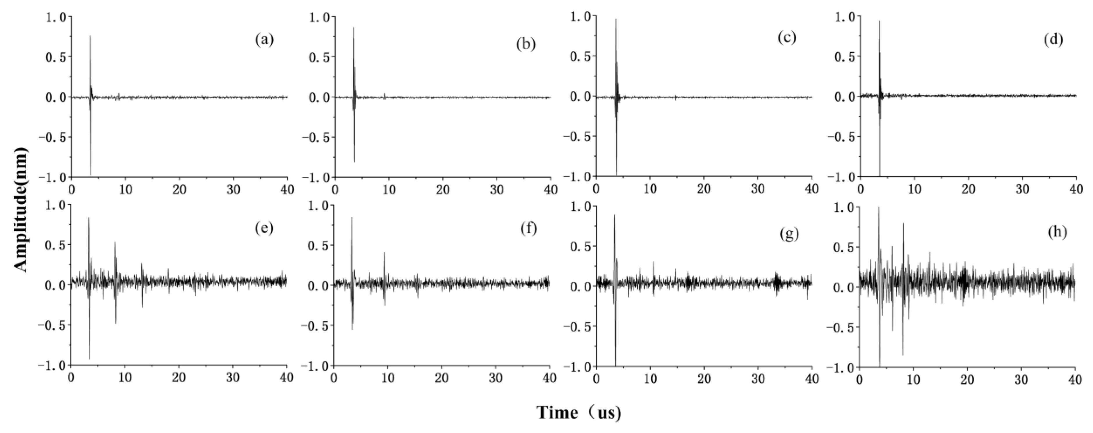
Using the laser-generated ultrasonics damage detection system, the ultrasonic responses of the aluminum alloy plates under the excitation of a single laser pulse were recorded and plotted in Figure 7.
4.2. Calculation of Embedding Parameters
The proposed technique attempts to detect the changes in the geometric figure in the state space resulting from damage. First, the baseline and current-line attractors are reconstructed by the response data recorded from both the undamaged and damaged structures. Notably, the attractors are reconstructed using the same embedding parameters. An accurate reconstruction requires a proper choice of embedding parameters, as mentioned above. Generally, the choice of the embedding dimension m should guarantee that the reconstructed attractor is unfolding in the state space. In addition, the choice of the time delay T depends on the appearance location of the first minimum value of the auto-covariance function. Here, the AMI function for time delay T and Cao’s function for dimension m are used. For the recorded response data x(n) (n = 1,2,…,N), the AMI quantifies the average amount of information obtained about x(n + T) through x(n). If x(n + T) and x(n) are completely independent, the AMI value becomes zero. However, in practice, the value of T corresponding to the first minimum of the AMI function is considered sufficient, which means that the first minimum value of T can be chosen as the proper time delay. Figure 8 shows the AMI values for the eight plates’ responses. When T reached 12, all the AMI values were reaching their minimum values. Hence, the time delay was chosen to be 12 for this experiment. A proper choice of embedding dimension m should guarantee that no false neighbors exist in the reconstructed state space. Cao’s functions for the eight plates’ responses are provided in Figure 9a. Figure 9b is Cao’s function for the plate whose minimum embedding dimension is largest compared with the others’. E1 and E2 are two quantities defined by Cao [29] for determining the minimum embedding dimension of a scalar time series. Suppose a time series, x1, x2, …,xN. The attractor Xi(m)can be reconstructed as follows [29]:
Define:
where ||·|| is some measurement of Euclidian distance and is given by the maximum norm, i.e.,
Define:
Then
Define:
Then
Equations (10) and (12) are the definitions of E1 and E2, respectively. Notably, the values of E1 and E2 stopped changing after m exceeded 15 and an embedding dimension of 16 was selected for this experiment. The detailed selection procedure can be found in [29].
4.3. Damage-Sensitive Feature: NNPE
Once the embedding parameters are selected, all segments with the same embedding parameters are used to reconstruct the attractors. Then, the NNPE values for the ultrasonic responses of specimens (b)–(h) are calculated by comparing their attractors with the reference undamaged attractor reconstructed from the ultrasonic response of specimen (a).
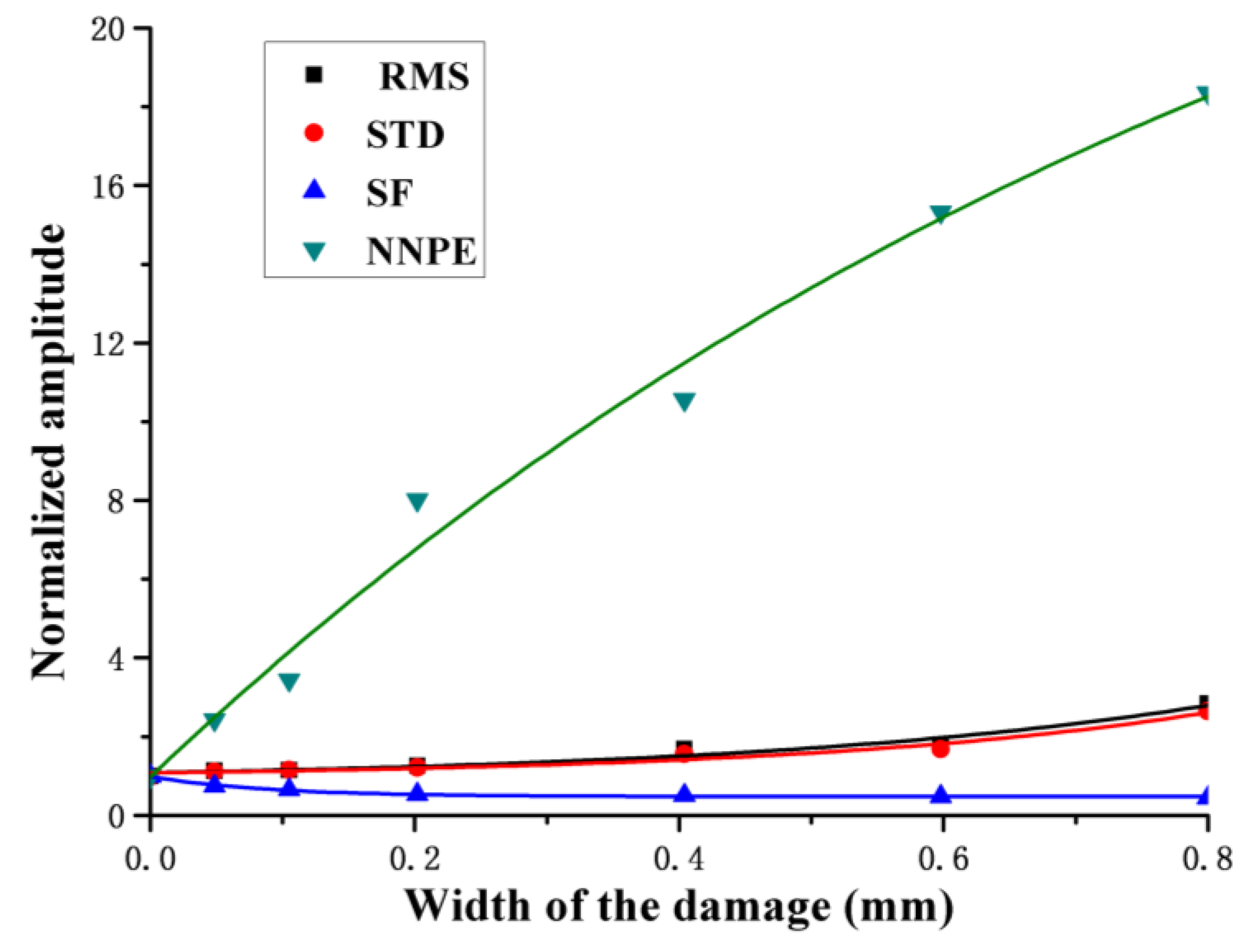
Several linear features, including the root mean square , standard deviation, and shape factor were calculated for the eight plates’ response data in addition to the NNPE values. These features are chosen not only for their ability to reflect the vibration amplitude and energy in the time domain but also for their power to represent the time series distribution of the responses [33]. To compare the performances of these features, all the calculation results are normalized by the undamaged value. The features can be calculated by the following equations:
where is the mean value of x(n).
Figure 10 shows the values of each feature calculated from the dynamic responses for specimens (b)–(h). It is clear that: (1) when the damage width exceeded 0.4 mm, all the feature values were changing, which means that all the features had the ability to detect damage larger than 0.4 mm; (2) the proposed linear features were relatively insensitive to damage smaller than 0.4 mm, as evidenced by the tangent slopes of the linear features’ plots that were close to zero when the damage was smaller than 0.4 mm; and (3) compared to the linear features, the plot of the NNPE had the steepest tangent slope when the damage width changed from 0 to 0.8 mm. The value of the tangent slope of the NNPE plot is almost 10 times larger than those of the others, especially when the damage width is smaller than 0.4 mm. This result reveals that the NNPE feature outperformed the other linear features and can be used to detect smaller damage.
4.4. Damage Visualization and Quantification
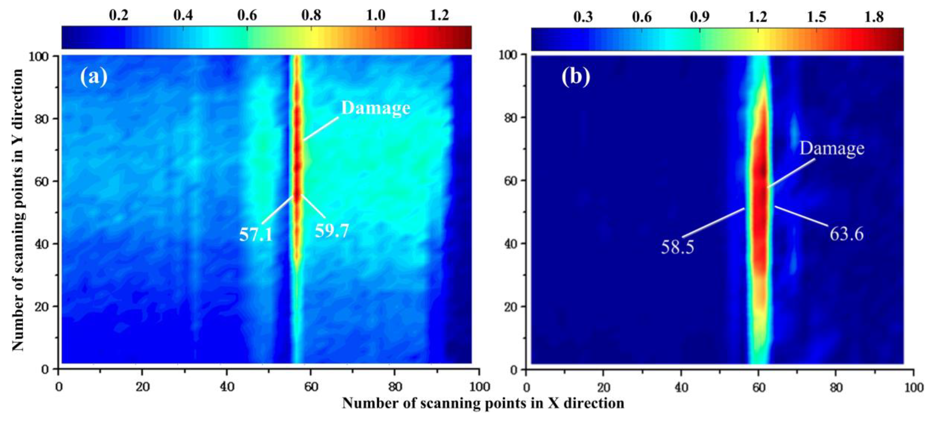
As mentioned in Section 2.3, the excitation laser pulse scans over both the damaged area and the comparison undamaged area while the ultrasonic responses from the excitation point are recorded by a transducer placed at a fixed point. The scanning area covering the damage was 5 × 5 mm2 in this experiment. The scanning process continues until the whole area is covered. The calculated NNPE values can be used to visualize the entire scanned area, and the spatial distribution of the values is expected to help in detecting the damage. Furthermore, because the pitch between two adjacent points in the scanned area is known before scanning (0.02 mm for this experiment), the size of the damage can be quantified by counting the number of points that contain damage in the visualization picture. The results are summarized in Figure 11. For simplicity’s sake, only the visualization pictures for specimens (c) and (d) with the smallest damage widths are plotted. One thing deserves to be mentioned is that when the laser beam spot irradiates in the front of the damage, the focal distance of the laser beam will change and result in a varying diameter of the laser beam spot. It means that the presence of the damage changes the characteristics of the structure as well as the laser beam. However, we should notice that the changing in the received signal caused by a varying laser beam spot is very limited. According to the work conducted by Aindow et al. [34], the diameter of the laser beam spot mainly affects the pulse duration of the surface waves. Compared with the nonlinear modulation caused by the damage as shown in Figure 2, the effects caused by a varying laser beam spot is almost negligible. From another perspective, the state-space predictive model mainly focuses on the changing of the received signal. Generally speaking, the changing of the laser beam spot caused by damage is helpful for the damage detection.
From Figure 11 we can see that a strongest nonlinearity was observed when damage appeared. Thus, the damage could be localized by the proposed technique successfully. Notably, the distribution of the damage is uniform through the Y direction. This is caused by the limitation of the transducer. When the laser pulse irradiates at the edge of the transducer, the laser generated ultrasonic waves will be propagating to the transducer obliquely. Some of the signals may be missed in this situation. So the calculated NNPE values are not uniformly distributed, especially at the edge of the scanning area. By extracting the coordinate values of the damage in Figure 11, the damage size can be quantified too. In Figure 11a, the longest distance of the damage width along the X direction was 59.7 − 57.1 = 2.6. The width of the damage was then 2.6 × 0.02 = 0.052 mm, which matched the actual width. Similarly, the width of the damage to structure (d) was 5.1 × 0.02 = 0.102 mm.
Using this method, the damage was not only localized, but its size was quantified too. Especially noteworthy is the number of scanning points and the pitches between two adjacent points being adjustable, which means, proper visualization parameters can be chosen to detect the different damage dimensions to obtain the best visualization results. For example, a larger distance between the scanning points should be chosen to visualize lager dimensioned damage.
In the above damage detection process, the crack is contained in the scanning area. However, if the damage is located between the scanning area and the transducer, the damage detection process is relatively cumbersome. In this situation, the detection process is as follows:
Three plates are needed, as shown in Figure 6a–c. Plates (a) and (b) are undamaged and plate (c) is a damaged plate with a crack. First of all, we make plate (a) the reference undamaged plate and plate (b) the current undamaged plate to be detected. Calculate the NNPE values in the scan area for plate (b). It is reasonable to predict that the calculated NNPE values will be basically the same. Secondly, make plate (a) the reference undamaged plate and plate (c) the current plate to be detected. Calculate the NNPE values in the scan area for plate (c). Again, the calculated NNPE values will be basically the same. Thirdly, compare the NNPE values calculated from plate (c) with the NNPE values calculated from plate (b). It is not hard to predict that the NNPE values calculated from plate (c) will be larger than the NNPE values calculated from plate (b) as a result of the damage. In this case, we can tell that there is a crack in plate (c), but the location of the crack is still unknown. This damage detection process is relatively cumbersome for practical applications. In the following, different scanning modes will be proposed to simplify the damage detection process.
5. Actual Damage Detection and Quantification of a Twin-Screw Compressor Body
5.1. Description of the Detection of a Twin-Screw Compressor Body
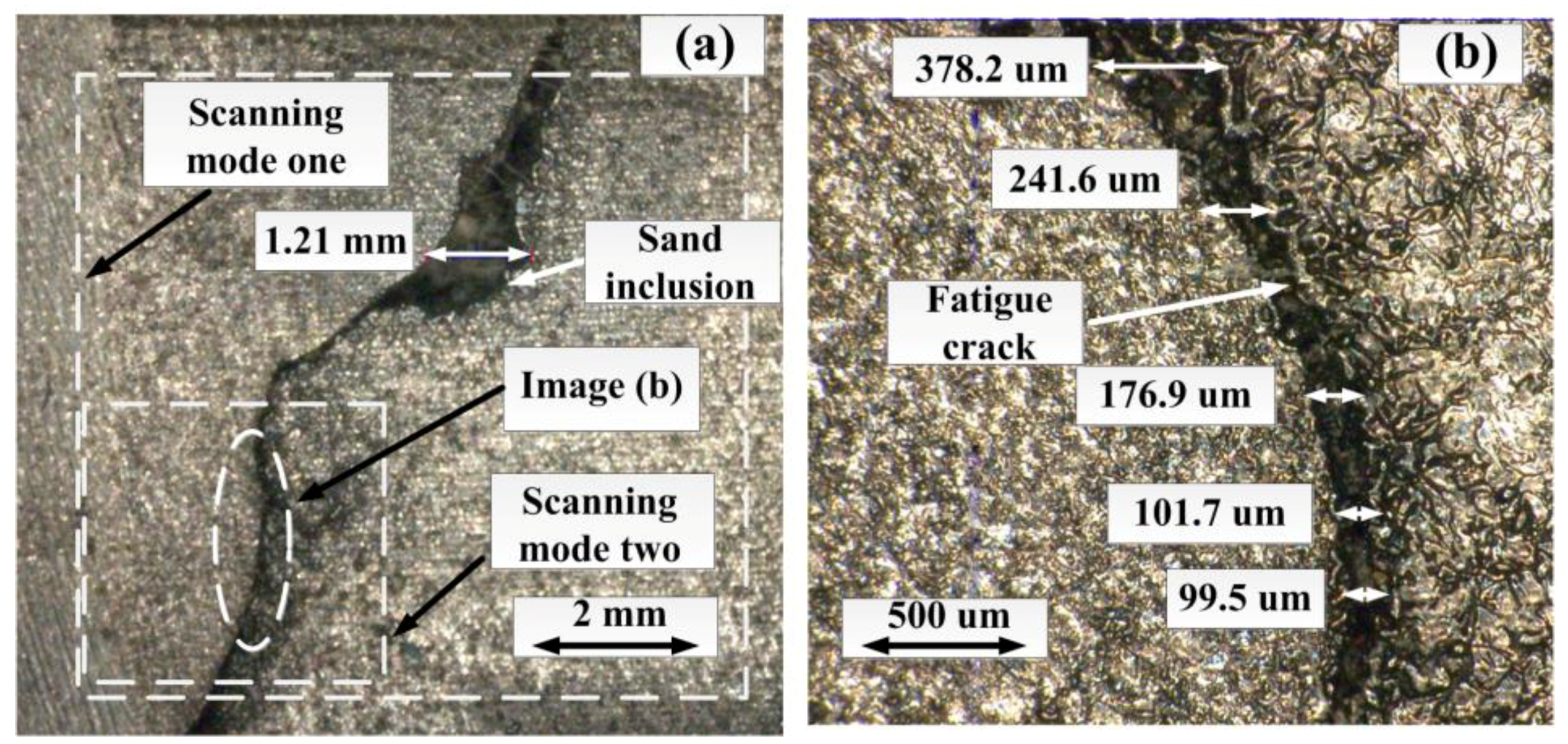
An actual 22 kW twin-screw compressor body (218A) is introduced for further verification of the effectiveness of the damage detection technique. The body is made of grey cast iron (No.35) by casting and has rough dimensions of 370 × 230 × 180 mm3, as shown in Figure 12. The upper and lower parts of the body are connected by positioning pins and bolts. There is a strict demand for the quality of the body because any small crack in the body may cause an extremely horrible production accident under high temperature and high-pressure working conditions. However, in practice, it is easy to produce sand inclusions and the resulting fatigue cracks into the body during the casting process. Using the proposed technique and the experimental setup proved in this study, the damage on the connection transverse plane was detected and quantified. Images of the actual damage are shown in Figure 13. Both images were taken with a digital microscope by KEYENCE (VHX-100). Figure 13a is a global view of the damage and contains both the sand inclusions and fatigue cracks. The magnification is 25 times the original size. Figure 13b is a local enlarged picture of Figure 13a. The area containing a fatigue crack in Figure 13a was extracted and enlarged to obtain a closer look at the damage. The magnification is 100 times the original size.
5.2. Damage Visualization and Quantification
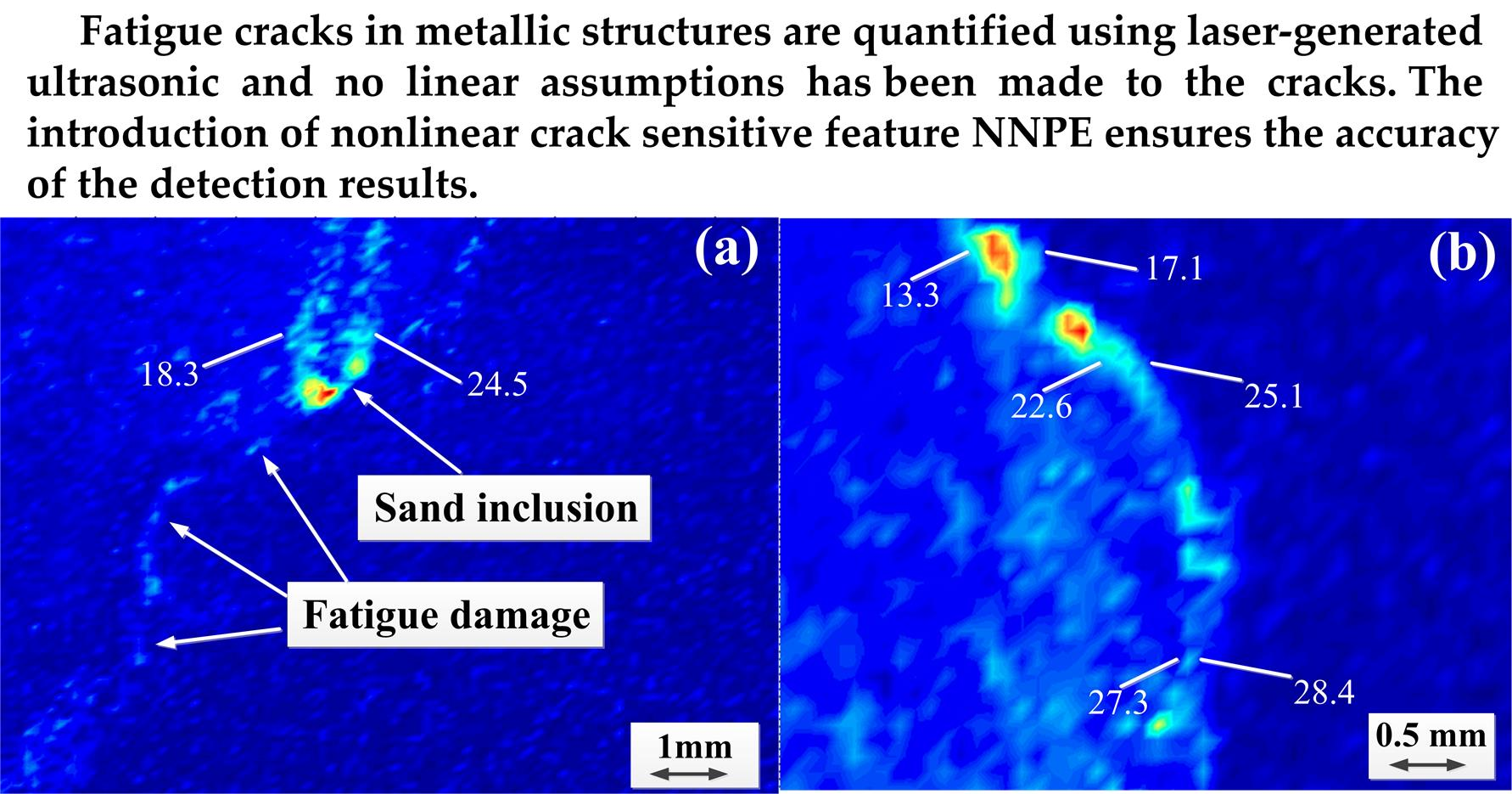
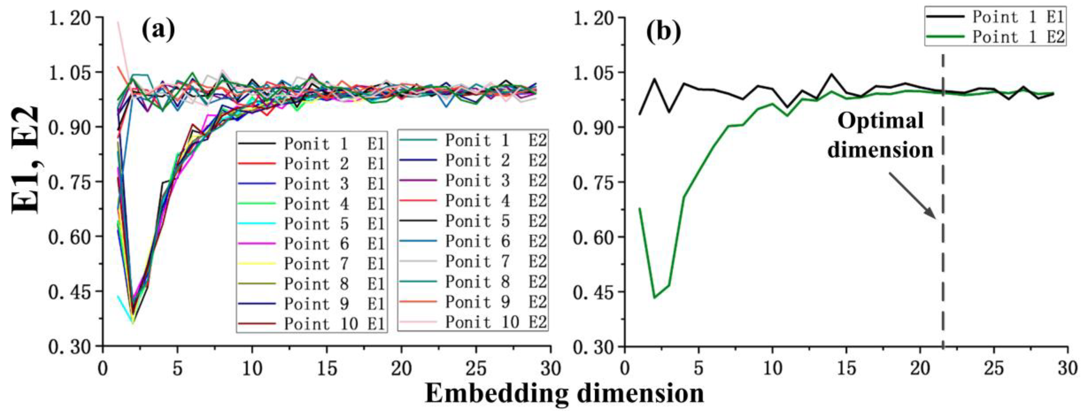
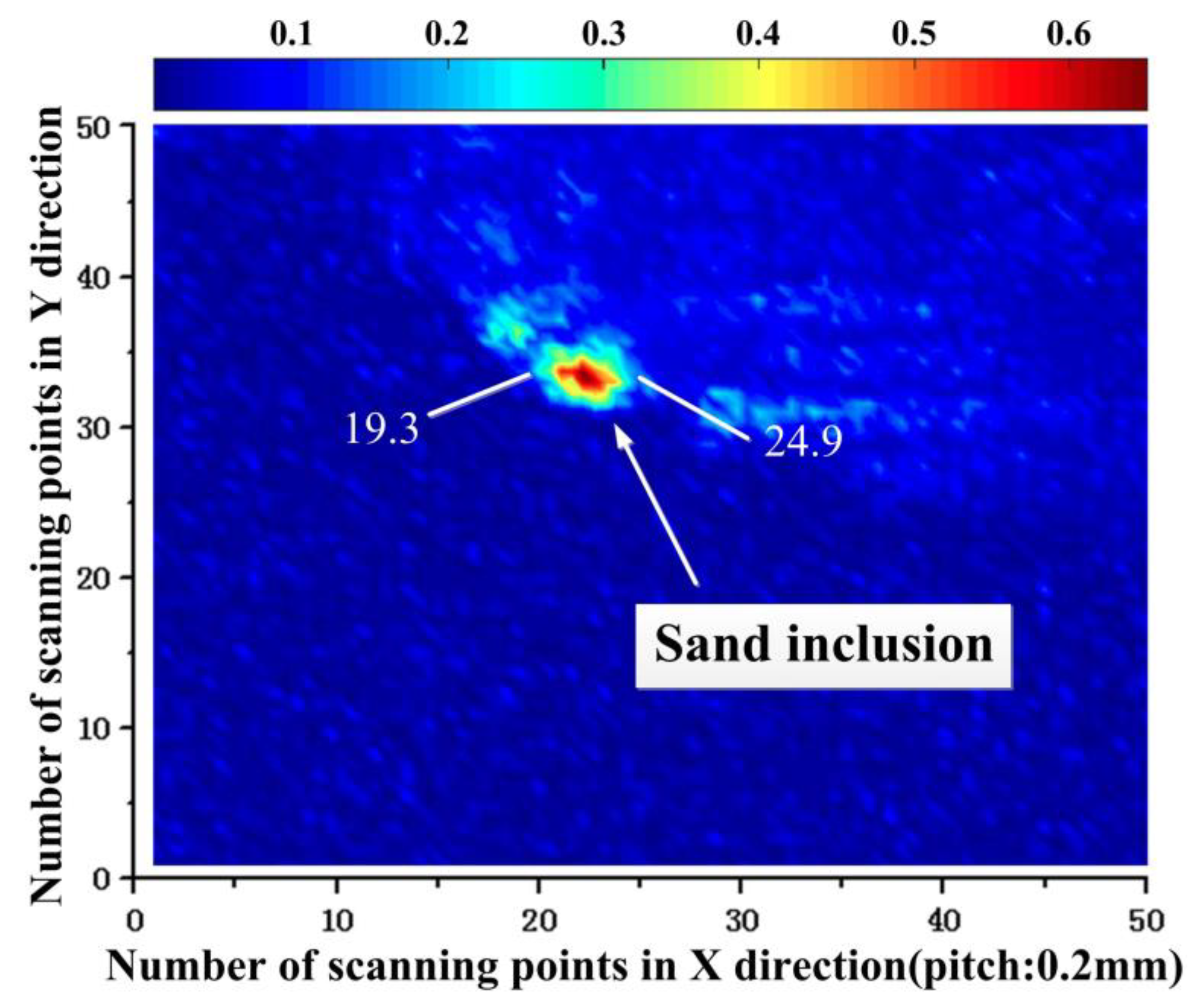
In this section, we discuss the detection, visualization and quantification of the damage on the connection transverse plane of a twin-screw compressor body using the experimental setup presented in Section 3. In this damage detection process, two scanning modes with different damage detection accuracies were used in the experiment to identify the damage with different dimensions. In mode one, the scanning area of the laser pulse was set to 10 × 10 mm2, and the distance between the two adjacent points was 0.2 mm, yielding 2500 scanning points. The damage was quickly located in this wide range scanning mode. The scanning area of the laser pulse was set to 5 × 5 mm2 in mode two. The distance between the two adjacent points was 0.1 mm, yielding 2500 scanning points. More information on the tiny damage was acquired by using this scanning mode. A schematic of the second scanning mode was shown in Figure 13a. In this experiment, the baseline data was acquired from the same connection transverse plane on the same twin-screw compressor body. The only difference is that the scanned area used for acquiring the baseline data was examined carefully with the digital microscope to make sure there is no obvious defect in the area. In this way, this area can be treated as the ‘reference undamaged structure’ in the experiment. The embedding parameters should be chosen before computing the NNPE values. The embedding parameters of ten randomly selected ultrasonic responses recorded by a transducer placed at a fixed point were calculated by the AMI and Cao’s function. The calculation results are provided in Figure 14 and Figure 15, respectively. The results calculated by Cao’s function for the response, whose minimum embedding dimension was the largest compared with those of the others, are shown in Figure 15b. From Figure 14 and Figure 15, when the time delay T reached 4, the calculation results for all the responses by using the AMI function were close to the minimum value, and the values of E1 and E2 did not change after m exceeded 23. Hence, T = 4 and m = 24 were selected in this experiment. Similarly, the time delay T and embedding dimension m in scanning mode two were calculated to be 3 and 19, respectively. Next, all responses with the same embedding parameters were used to reconstruct the attractors. Based on the attractors reconstructed from both the undamaged and damaged sections, the 2500 NNPE values were computed and are summarized in Figure 16. Here, the detection result by linear feature root mean square was also calculated as shown in Figure 17 in addition to the NNPE values. In Figure 16a, the values of the feature NNPE around the sand inclusion are the largest compared with others in the scanning area. Thus, the sand inclusion can be detected and visualized clearly. Furthermore, the shape and direction of the resulting fatigue crack can be vaguely distinguished from the picture too. But, the picture of the fatigue crack is almost submerged in the environmental noise due to the low detection accuracy. In Figure 16b, the shape and direction information of the fatigue crack can be identified clearly, which means that in scanning mode two the damage detection accuracy has been greatly improved as a result of changes in the visualization parameters. In Figure 17, the sand inclusion has been detected and visualized successfully. However, the detection of the resulting fatigue crack has failed since there is no obvious information about the fatigue crack in Figure 17. This detection result is not surprised since the nonlinear ultrasonic features are usually more sensitive to small cracks than the linear ones as mentioned above. This detection result is consistent with the result given in Figure 10.
By extracting the coordinate values of the damage, the size of the cracks can also be quantified. The largest width of the sand inclusion in Figure 16 was 1.24(0.2 × (24.5 − 18.3)) mm. The largest width of the sand inclusion in Figure 17 was 1.12 (0.2 × (24.9 − 19.3)) mm. Both of the calculated values were in line with its actual size of 1.21 mm, but the value calculated by NNPE values is more accurate. The widths of the measuring points in Figure 16b are 380 (0.1 × (17.1 − 13.3)) um, 250 (0.1 × (25.1 − 22.6)) um, and 110 (0.1 × (28.4 − 27.3)) um, respectively, which match the actual measurements well. Therefore, the proposed technique was again able to detect and quantify the damage on the connection transverse plane of the twin-screw compressor body. Also from the result we can see that the nonlinear feature NNPE is more sensitive to the damage than the linear feature.
6. Conclusions
This paper presents a non-destructive damage detection, visualization, and quantification technique based on laser-generated ultrasonics and state-space predictive models. Different types of damage to aluminum alloy plates and a twin-screw compressor body were detected and quantified by using NNPE. This feature is extracted from the attractors reconstructed by the ultrasonic responses in the time domain recorded by a transducer mounted at the surface of the structure. By capturing the differences in the NNPE values between the undamaged and damaged structures, the nonlinearity of the structures, which are usually caused by damage, can be detected. Furthermore, the damage can be visualized and even quantified by observing the spatial distribution of NNPE values calculated by the ultrasonic responses from the area excited by a scanning laser pulse. Artificial damage to aluminum alloy plates, as well as the actual sand inclusions and fatigue cracks in a twin-screw compressor body, have been successfully detected and quantified by using the proposed technique.
Some important issues that are not considered in this paper are the capability of the technique in detecting the depth of the damage, the internal damage, and the damage on curved surface. A follow-up study with the proposed feature NNPE will focus on those issues.
Author Contributions
Y.L. and S.Y. conceived and designed the experiments; Y.L. and X.L. performed the experiments; Y.L. and X.L. analyzed the data; Y.L. contributed reagents/materials/analysis tools; Y.L. wrote the paper.
Acknowledgments
This research was funded by National Natural Science Foundation of China under Grant Number 51375434.
Conflicts of Interest
The authors declare no conflict of interest.
References
- Chatterjee, A.; Kotambkar, M.S. Modal characteristics of turbine blade packets under lacing wire damage induced mistuning. J. Sound Vib. 2015, 343, 49–70. [Google Scholar] [CrossRef]
- Ukar, E.; Lamikiz, A.; Martínez, S.; Tabernero, I.; López De Lacalle, L.N. Roughness prediction on laser polished surfaces. J. Mater. Process. Technol. 2012, 212, 1305–1313. [Google Scholar] [CrossRef]
- Suárez, A.; Veiga, F.; López De Lacalle, L.N.; Polvorosa, R.; Lutze, S.; Wretland, A. Effects of ultrasonics-assisted face milling on surface integrity and fatigue life of Ni-Alloy 718. J. Mater. Eng. Perform. 2016, 25, 5076–5086. [Google Scholar]
- Campbell, F.C. Elements of Metallurgy and Engineering Alloys; ASM International: Novelty, OH, USA, 2008. [Google Scholar]
- Lee, C.; Kim, J.; Park, S.; Kim, D.H. Advanced fatigue crack detection using nonlinear self-sensing impedance technique for automated NDE of metallic structures. Res. Nondestruct. Eval. 2015, 26, 107–121. [Google Scholar] [CrossRef]
- Calleja Ochoa, A.; González Barrio, H.; Polvorosa Teijeiro, R.; Ortega Rodríguez, N.; López-de-Lacalle, L.N. Multitasking machines: Evolution, resources, processes and scheduling. DYNA 2017, 92, 637–642. [Google Scholar]
- Burleigh, D.; Vavilov, V.P.; Pawar, S.S. The influence of optical properties of paints and coatings on the efficiency of infrared nondestructive testing applied to aluminum aircraft structures. Infrared Phys. Technol. 2016, 77, 230–238. [Google Scholar] [CrossRef]
- Kim, D.; Udpa, L.; Udpa, S. Remote field eddy current testing for detection of stress corrosion cracks in gas transmission pipelines. Mater. Lett. 2004, 58, 2102–2104. [Google Scholar] [CrossRef]
- Teitsma, A.; Takach, S.; Maupin, J.; Fox, J.; Shuttleworth, P.; Seger, P. Small diameter remote field eddy current inspection for unpiggable pipelines. J. Press. Vessel Technol. 2005, 127, 269–273. [Google Scholar] [CrossRef]
- Krenkel, W.; Heidenreich, B.; Renz, R. C/C-SiC composites for advanced friction systems. Adv. Eng. Mater. 2002, 4, 427–436. [Google Scholar] [CrossRef]
- Zhang, Y.; Li, D.; Zhou, Z. Time reversal method for guided waves with multimode and multipath on corrosion defect detection in wire. Appl. Sci. 2017, 7, 424. [Google Scholar] [CrossRef]
- Worden, K.; Farrar, C.R.; Haywood, J.; Todd, M. A review of nonlinear dynamics applications to structural health monitoring. Struct. Control Health Monit. 2008, 15, 540–567. [Google Scholar] [CrossRef]
- Jiao, J.P.; Zheng, L.; Song, G.R.; He, C.; Wu, B. Vibro-acoustic modulation technique for micro-crack detection in pipeline. In Proceedings of the 7th International Symposium on Precision Engineering Measurements and Instrumentation, Lijiang, China, 7–11 August 2011. [Google Scholar]
- Duffour, P.; Morbidini, M.; Cawley, P. Comparison between a type of vibro-acoustic modulation and damping measurement as NDT techniques. NDT & E Int. 2006, 39, 123–131. [Google Scholar]
- Liu, P.; Sohn, H.; Jeon, I. Nonlinear spectral correlation for fatigue crack detection under noisy environments. J. Sound Vib. 2017, 400, 305–316. [Google Scholar] [CrossRef]
- Hess, P.; Lomonosov, A.M.; Mayer, A.P. Laser-based linear and nonlinear guided elastic waves at surfaces (2D) and wedges (1D). Ultrasonics 2014, 54, 39–55. [Google Scholar] [CrossRef] [PubMed]
- Gusev, V.; Chigarev, N. Nonlinear frequency-mixing photoacoustic imaging of a crack: Theory. J. Appl. Phys. 2010, 107, 124905. [Google Scholar] [CrossRef]
- Chigarev, N.; Zakrzewski, J.; Tournat, V. Nonlinear frequency-mixing photoacoustic imaging of a crack. J. Appl. Phys. 2009, 106, 036101. [Google Scholar] [CrossRef]
- Liu, P.; Sohn, H. Damage detection using sideband peak count in spectral correlation domain. J. Sound Vib. 2017, 411, 20–33. [Google Scholar] [CrossRef]
- Yoder, N.C.; Adams, D.E. Vibro-acoustic modulation utilizing a swept probing signal for robust crack detection. Struct. Health Monit. Int. J. 2010, 9, 257–267. [Google Scholar] [CrossRef]
- White, R.M. Generation of elastic waves by transient surface heating. J. Appl. Phys. 1963, 34, 3559–3569. [Google Scholar] [CrossRef]
- Nichols, J.M. Structural health monitoring of offshore structures using ambient excitation. Appl. Ocean Res. 2003, 25, 101–114. [Google Scholar] [CrossRef]
- Martínez, S.; Lamikiz, A.; Ukar, E.; Calleja, A.; Arrizubieta, J.A.; López De Lacalle, L.N. Analysis of the regimes in the scanner-based laser hardening process. Opt. Lasers Eng. 2017, 90, 72–80. [Google Scholar] [CrossRef]
- Overbey, L.A.; Olson, C.C.; Todd, M.D. A parametric investigation of state-space-based prediction error methods with stochastic excitation for structural health monitoring. Smart Mater. Struct. 2007, 16, 1621–1638. [Google Scholar] [CrossRef]
- Liu, G.; Mao, Z.; Todd, M.; Huang, Z. Localization of nonlinear damage using state-space-based predictions under stochastic excitation. Smart Mater. Struct. 2014, 23, 025036. [Google Scholar] [CrossRef]
- Liu, G.; Mao, Z.; Todd, M. Damage detection using transient trajectories in phase-space with extended random decrement technique under non-stationary excitations. Smart Mater. Struct. 2016, 25, 115014. [Google Scholar] [CrossRef]
- Takens, F. Detecting Strange Attractors in Turbulence, in Dynamical Systems and Turbulence; Springer: Berlin/Heidelberg, Germany, 1981; pp. 366–381. [Google Scholar]
- Fraser, A.M.; Swinney, H.L. Independent coordinates for strange attractors from mutual information. Phys. Rev. A 1986, 33, 1134–1140. [Google Scholar] [CrossRef]
- Cao, L.Y. Practical method for determining the minimum embedding dimension of a scalar time series. Phys. D Nonlinear Phenom. 1997, 110, 43–50. [Google Scholar] [CrossRef]
- Pecora, L.M.; Carroll, T.L. Discontinuous and non-differentiable functions and dimension increase induced by filtering chaotic data. Chaos 1996, 6, 432–439. [Google Scholar] [CrossRef] [PubMed]
- Overbey, L.A.; Todd, M.D. Damage Assessment using generalized state-space correlation features. Struct. Health Monit. Int. J. 2008, 7, 347–363. [Google Scholar] [CrossRef]
- Nichols, J.M.; Todd, M.D.; Wait, J.R. Using state space predictive modeling with chaotic interrogation in detecting joint preload loss in a frame structure experiment. Smart Mater. Struct. 2003, 12, 580–601. [Google Scholar] [CrossRef]
- Lei, Y.G.; He, Z.J.; Zi, Y.Y.; Chen, X. New clustering algorithm-based fault diagnosis using compensation distance evaluation technique. Mech. Syst. Signal Process. 2008, 22, 419–435. [Google Scholar] [CrossRef]
- Aindow, A.; Dewhurst, R.J.; Hutchins, D.A.; Palmer, S.B. Characteristics of a laser-generated acoustic source in metals. In Proceedings of the European Conference on Optical Systems and Application, Utrecht, The Netherlands, 23–25 September 1980; Volume 236, pp. 478–485. [Google Scholar]
Figure 1.
The illustration of nonlinear modulation of two ultrasonic waves.

Figure 2.
The illustration of laser-generated ultrasonics modulations.
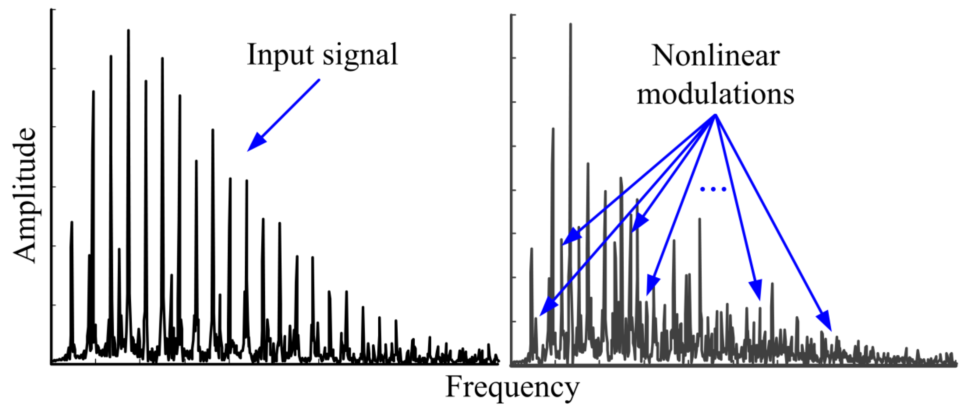
Figure 3.
The schematic of feature extraction.

Figure 4.
The schematic diagram of the damage detection technique.

Figure 5.
The schematic diagram of the laser-generated ultrasonics detection system; 1: Laser generator; 2: Galvanometric scanner; 3: Structure to be tested; 4: Transducer; 5:Three-dimensional transition stage; 6: Data acquisition system; 7: Data processing system.
Figure 5.
The schematic diagram of the laser-generated ultrasonics detection system; 1: Laser generator; 2: Galvanometric scanner; 3: Structure to be tested; 4: Transducer; 5:Three-dimensional transition stage; 6: Data acquisition system; 7: Data processing system.

Figure 6.
The dimension of the plates, damage, laser excitation, and detection arrangement:(a) Reference undamaged plate; (b) currently undamaged plate;(c)damage width: 0.05 mm; (d) damage width: 0.1 mm; (e) damage width: 0.2 mm; (f) damage width: 0.4 mm; (g) damage width: 0.6 mm; (h) damage width: 0.8 mm.
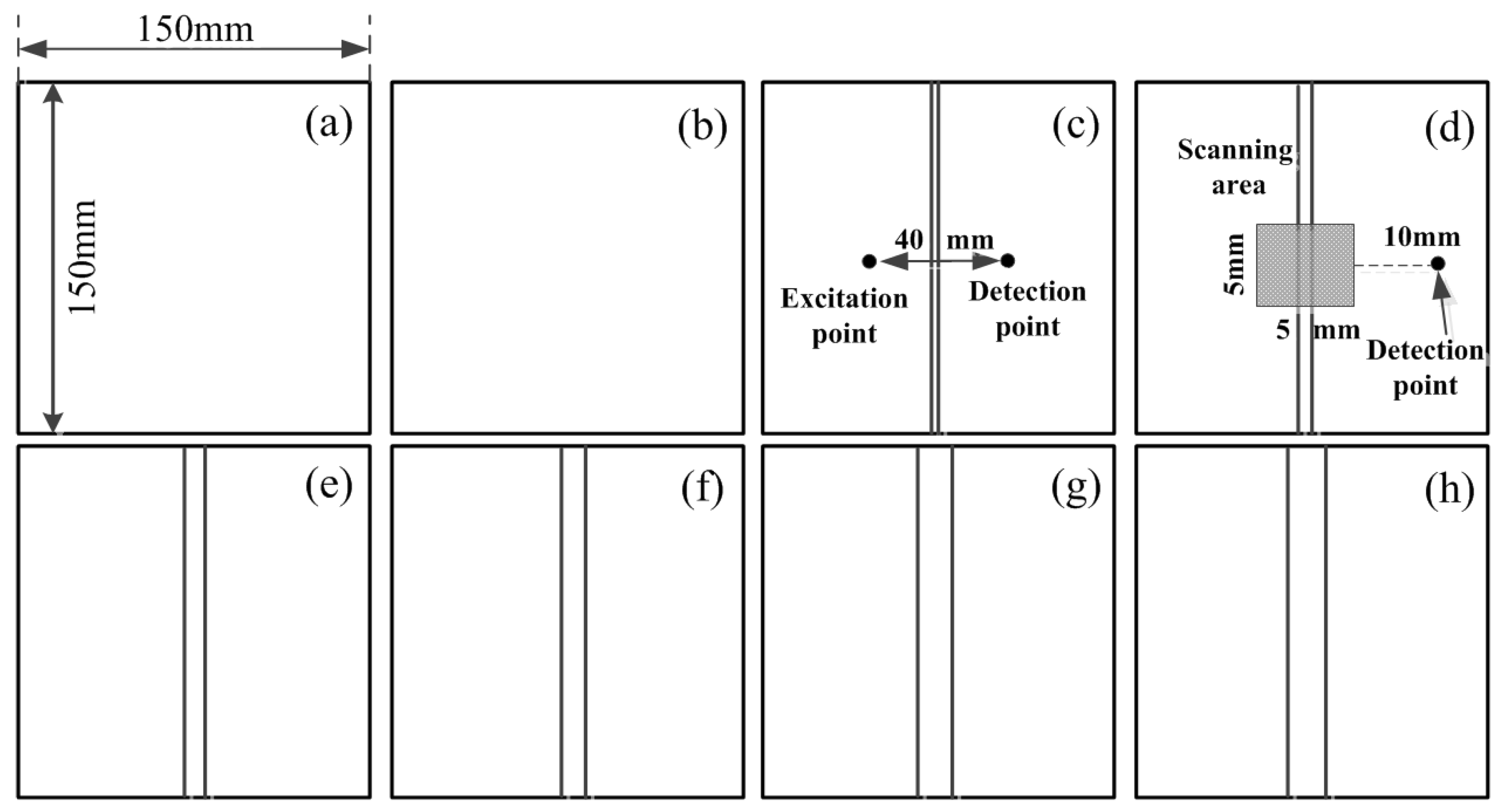
Figure 7.
The recorded ultrasoinc responses in the time domain: (a) Reference undamaged plate; (b) currently undamaged plate;(c)damage width: 0.05 mm; (d) damage width: 0.1 mm; (e) damage width: 0.2 mm; (f) damage width: 0.4 mm; (g) damage width: 0.6 mm; (h) damage width: 0.8 mm.
Figure 7.
The recorded ultrasoinc responses in the time domain: (a) Reference undamaged plate; (b) currently undamaged plate;(c)damage width: 0.05 mm; (d) damage width: 0.1 mm; (e) damage width: 0.2 mm; (f) damage width: 0.4 mm; (g) damage width: 0.6 mm; (h) damage width: 0.8 mm.

Figure 8.
The average mutual information (AMI) function for time delay T.
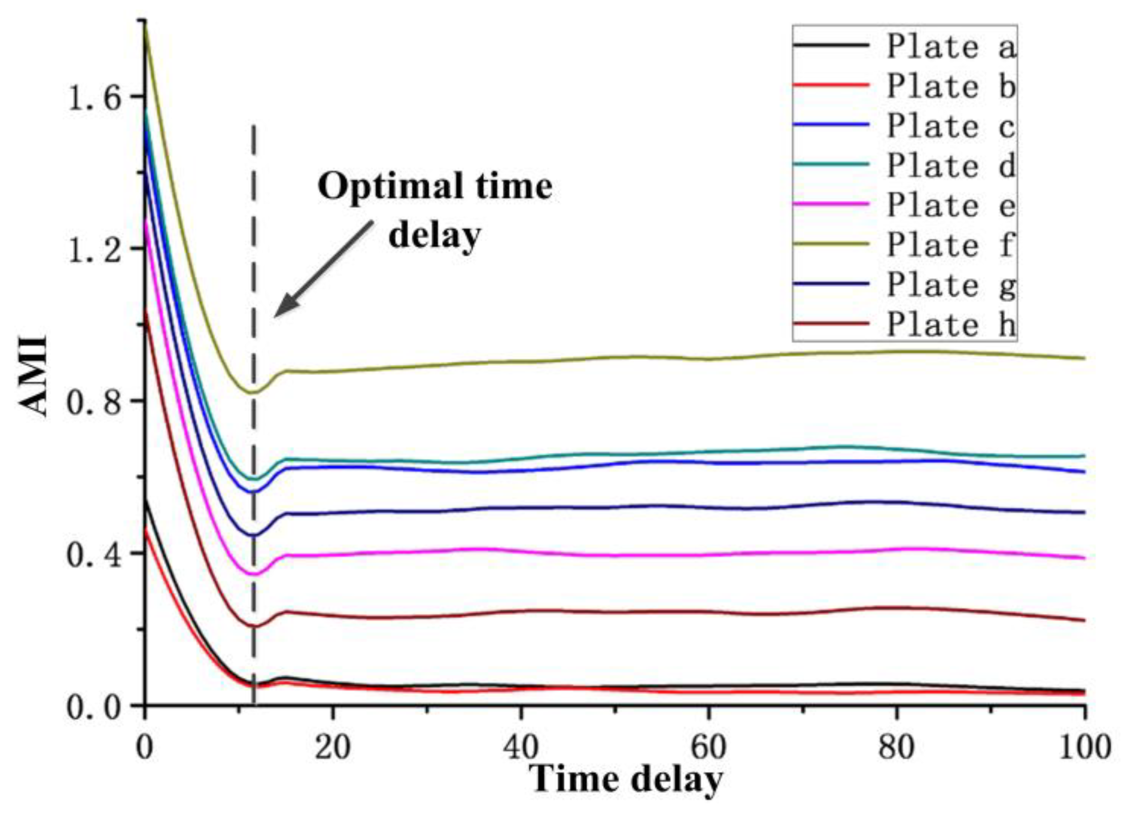
Figure 9.
Cao’s function for embedding dimension m: (a) Cao’s function for the eight plates’ responses; (b) Cao’s function for the plate with the largest embedding dimension.
Figure 9.
Cao’s function for embedding dimension m: (a) Cao’s function for the eight plates’ responses; (b) Cao’s function for the plate with the largest embedding dimension.
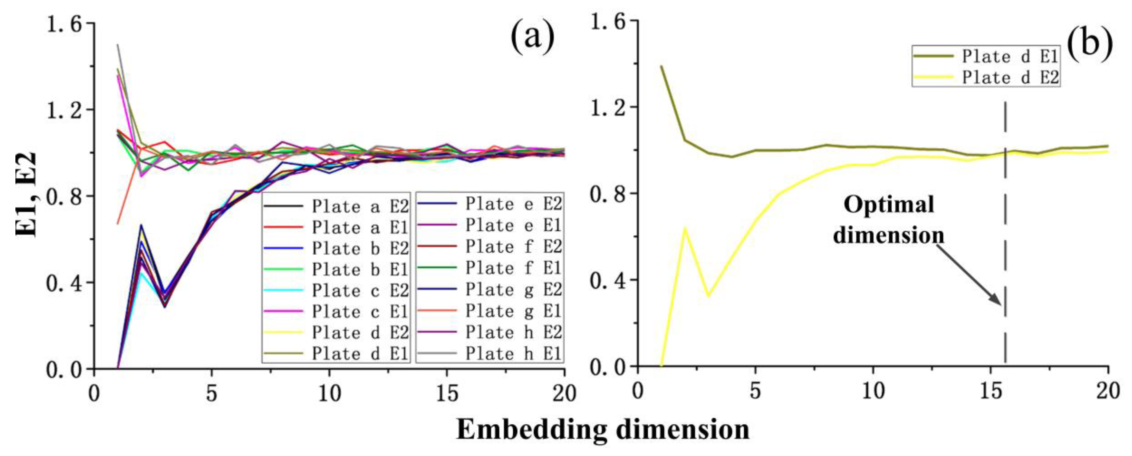
Figure 10.
A comparison of the normalized features at different damage widths.

Figure 11.
Damage visualization by the NNPE values: (a) Damage width: 0.05 mm; (b) damage width: 0.1 mm.
Figure 11.
Damage visualization by the NNPE values: (a) Damage width: 0.05 mm; (b) damage width: 0.1 mm.

Figure 12.
The twin-screw compressor body.
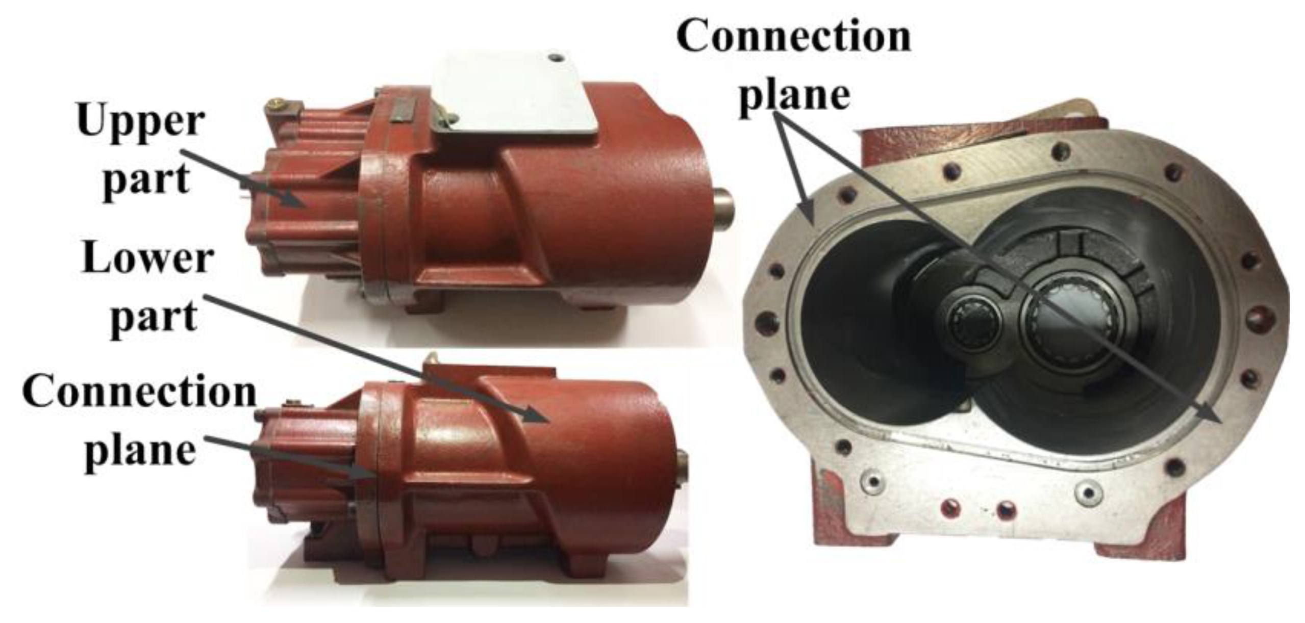
Figure 13.
The images of the damage in two different scanning modes: (a) a global view of the damage; (b) enlarged local fatigue crack.
Figure 13.
The images of the damage in two different scanning modes: (a) a global view of the damage; (b) enlarged local fatigue crack.

Figure 14.
The AMI versus time delay T.
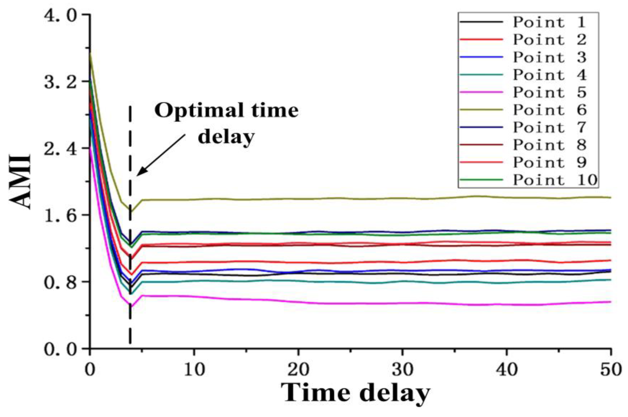
Figure 15.
The Cao’s function versus the embedding dimension m: (a) Cao’s function for the ten randomly selected ultrasonic responses; (b) Cao’s function for the ultrasonic response with the largest embedding dimension.
Figure 15.
The Cao’s function versus the embedding dimension m: (a) Cao’s function for the ten randomly selected ultrasonic responses; (b) Cao’s function for the ultrasonic response with the largest embedding dimension.

Figure 16.
The damage visualization by the NNPE values (the pitches between the two adjacent points are: (a) 0.2 mm; (b) 0.1 mm.
Figure 16.
The damage visualization by the NNPE values (the pitches between the two adjacent points are: (a) 0.2 mm; (b) 0.1 mm.
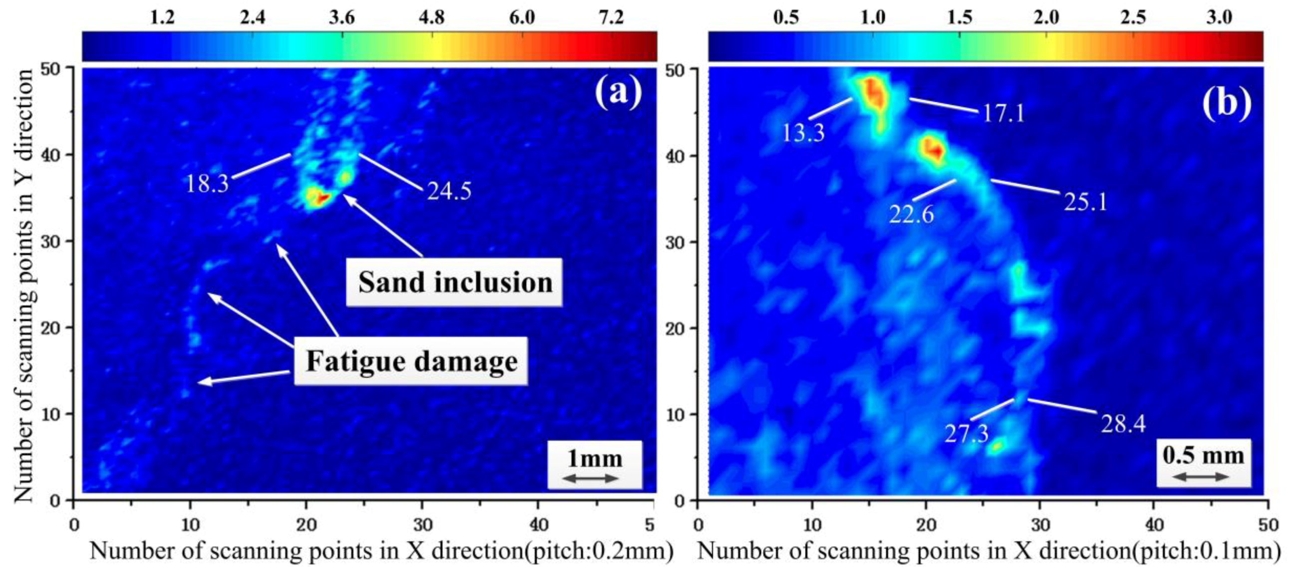
Figure 17.
The damage visualization by the linear RMS values.
© 2018 by the authors. Licensee MDPI, Basel, Switzerland. This article is an open access article distributed under the terms and conditions of the Creative Commons Attribution (CC BY) license (http://creativecommons.org/licenses/by/4.0/).
Share and Cite
MDPI and ACS Style
Liu, Y.; Yang, S.; Liu, X. Detection and Quantification of Damage in Metallic Structures by Laser-Generated Ultrasonics. Appl. Sci. 2018, 8, 824. https://doi.org/10.3390/app8050824
AMA Style
Liu Y, Yang S, Liu X. Detection and Quantification of Damage in Metallic Structures by Laser-Generated Ultrasonics. Applied Sciences. 2018; 8(5):824. https://doi.org/10.3390/app8050824
Chicago/Turabian StyleLiu, Yongqiang, Shixi Yang, and Xuekun Liu. 2018. "Detection and Quantification of Damage in Metallic Structures by Laser-Generated Ultrasonics" Applied Sciences 8, no. 5: 824. https://doi.org/10.3390/app8050824
Note that from the first issue of 2016, this journal uses article numbers instead of page numbers. See further details here.