Analysis of Blur Measure Operators for Single Image Blur Segmentation


School of Computer Science and Engineering, Korea University of Technology and Education, 1600 Chungjeolno, Byeogchunmyun, Cheonan 31253, Korea
*
Author to whom correspondence should be addressed.
Appl. Sci. 2018, 8(5), 807; https://doi.org/10.3390/app8050807
Submission received: 31 March 2018
/
Revised: 12 May 2018
/
Accepted: 14 May 2018
/
Published: 17 May 2018
Abstract
:Blur detection and segmentation for a single image without any prior information is a challenging task. Numerous techniques for blur detection and segmentation have been proposed in the literature to ultimately restore the sharp images. These techniques use different blur measures in different settings, and in all of them, blur measure plays a central role among all other steps. Blur measure operators have not been analyzed comparatively for both of the spatially-variant defocus and motion blur cases. In this paper, we provide the performance analysis of the state-of-the-art blur measure operators under a unified framework for blur segmentation. A large number of blur measure operators are considered for applying on a diverse set of real blurry images affected by different types and levels of blur and noise. The initial blur maps then are segmented into blurred and non-blurred regions. In order to test the performance of blur measure operators in segmentation process in equal terms, it is crucial to consider the same intermediate steps involved in the blur segmentation process for all of the blur measure operators. The performance of the operators is evaluated by using various qualitative measures. Results reveal that the blur measure operators perform well under certain condition and factors. However, it has been observed that some operators perform adequately overall well or worse against almost all imperfections that prevail over the real-world images.
1. Introduction
Blur in images is considered as an undesirable effect because it leads to the loss of the necessary details required for the scene interpretation. Automatic detection of blurred and sharp pixels in an image and their classification into respective regions are very important for different image processing and computer vision applications [1]. The benefits of blur segmentation are exhibited in many applications including but not limited to object detection [2], scene classification [3], image segmentation [4], background blur magnification [5], depth of field extension [6] and depth estimation [7,8]. Blur detection and segmentation for a single image without any prior information is a challenging task.
For blur detection and segmentation, a large number of techniques have been proposed in the literature [9,10,11,12,13,14,15,16,17]. The blur segmentation techniques comprise of a number of key steps. The first and the fundamental step is to employ a blur measure (BM) operator which measures the level of blurriness associated with the pixels or regions of the image and realizes discrimination between sharp and blurred pixels or regions of the image is realized by applying an operator, known as blur measure (BM) operator. In the second step, the features computed through the BM operator(s) are provided to a classifier for segmentation of the blurred and sharp regions. Finally, various postprocessing techniques are deployed for improve the initial segmentation results. In each of the techniques, the quality of the underlying blur measure operator plays a distinguishing role. Recently, Lai et al. [18] reported that the existing techniques perform well on images with certain properties however, their performance is deteriorated in real images. As different blur measure operators recognize and exploit different features of the input blurred image, it is difficult to determine which operator has the best performance under which conditions. Additionally, due to the diversity in the subsequent steps of segmentation process, it becomes unjustifiable to compare the output of one BM operator with that of another one.
In this paper, we aim for a comprehensive study to analyze the performance of the state-of-the-art blur measure operators used to detect and segment blurred and sharp regions of the image. In our study, the performance of recently suggested BM’s is investigated. In addition, a number of operators which have also been studied in this work were originally developed for autofocus and shape from focus (SFF) techniques [19]. They have been brought into this study because their working principle is similar to that of blur measure operators i.e., each of them can distinguish between sharp and blurred regions of the image by manifesting different responses for these different regions. For experiments, we have considered a dataset of real-world blurred images with the diverse levels and types of blur. A number of experiments have been conducted on the sample images for qualitative and quantitative results which have been presented accordingly. The statistical evaluation of different blur measure operators helps to understand their prospective performance attributes.
The rest of the paper is organized as follows. The Section 2 sheds light on the related work done in the past. Section 3 explains the methodology for the blur segmentation, including image data sets, blur measure operators and the evaluation measures. Experimental results and analysis are presented in Section 4. Finally, the work is concluded by Section 5.
2. Related Work
Most of the images captured using optical imaging systems usually contain two types of the regions: blurred and sharp. Blur can be categorized mainly into two types: (a) defocus blur, which is caused by the optical imaging system and (b) motion blur, which is caused by the relative motion between camera and scene objects. Blur in the image causes the deterioration of the image quality in that region. Therefore, it is important to detect and eliminate the blur from the images.
Blur detection techniques can be divided broadly into two classes: (1) techniques that need only one image [9,10,11,12,13,14,15] and (2) techniques that use multiple images [20,21]. Though, high-quality image can be recovered through multi-image scheme, yet it is a very challenging task as it requires to align the images, and thus it poses concerns on its applicability. Moreover, our study is restricted to techniques for single image. Shi et al. differentiate between blurred and sharp regions based on the features like image gradient, spectra in frequency domain and data driven local filters in a multiscale scheme [11]. Bae and Durand focused on the blurriness of the edge pixels by employing multiscale edge detector and then propagated this measure to the rest of the image [5]. Elder and Zucker measured the image blur by calculating first and second order gradients on the edges [22]. Namboodiri and Chaudhuri employed the inhomogenous inversion heat diffusion to measure the defocus blur on the edges and propagated them through graph-cuts [23]. Tai and Brown estimated the defocus blur in [24] by using a local contrast prior on edge gradient magnitudes and then propagated through Markov random field (MRF). Zhuo and Sim looked for the Gaussian blur on edge pixels and then interpolated through matting Laplacian for non-edge pixels [25]. Peng et al. measured the pixel blur by calculating the difference between before and after multi-scale Gaussian smoothing [26]. Then, blur map is refined by employing morphological reconstruction and guided filtering. Zhang and Hirakawa measured the blurriness by exploiting the double discrete wavelet transform [27]. Zhu et al. used localized Fourier spectrum to measure the probability of blur scale for each pixel and then implemented a constrained pairwise energy function [28]. Shi et al. estimated the slight noticeable blur by utilizing sparse representation of image neighborhood windows in dictionary method and this blur is further smoothed by an edge-preserving fitler [12]. Lin et al. estimated local blur by analyzing local and global gradient statistics [29]. Oliveira et al. restored the natural images through their spectrum by estimating the parameters for defocus and motion blur kernels [30]. Tang et al. proposed a general framework to retrieve a course blur map for both defocus and motion blurred images by using the log averaged spectrum residual of the image, and then updated it iteratively to achieve the fine map by exploiting the intrinsic relevance of the neighboring similar regions of the image [13]. Yi and Eramian proposed a blur measure operator based on the difference between the distributions of uniform local binary patterns (LBP) of the blurred and proposed a robust algorithm to segment the defocus blur [14]. Golestaneh and Karam detected the spatially varying blur by applying multiscale fusion of the high frequency Discrete Cosine Transform (DCT) coefficients [31]. Chakrabarti et al. used a mixture of Gaussians to model the heavy-tailed natural image gradients and estimated the likelihood of spatially varying directional motion blur in the image using local Fourier transform [32].
Spatially uniform motion deblurring techniques are discussed in [33,34,35,36,37,38]. Most of the uniform deblurring techniques have difficulty in handling non-uniform blurred images. Pan et al. and Hyun et al. have discussed the problem of motion deblurring for general dynamic scenes in which object motion and camera shake both are involved [33,34]. Now, we mention spatially non-uniform camera motion deblurring techniques. Whyte et al. simplified a general projective model proposed by [39] and employed a variational Bayesian framework for image deblurring [35]. Gupta et al. utilized motion density functions to estimate the camera motion trajectory [36]. Shan et al. analyzed the rotational motion blur using a transparency map [38]. Generally, it is computationally expensive if optimization is to be applied in any of these non-uniform deblurring techniques. To tackle it, neighborhood window-based locally uniform techniques are developed which involve fast Fourier transform to provide computationally efficient results. These techniques are to counter for the camera motion [37].
In the following paragraphs, we highlight the spatially non-uniform object motion deblurring techniques. Raskar et al. [40] removed the motion blur by preserving the high frequency content of the imaged scene by fluttering the camera’s shutter open and close during the exposure time according to a well chosen binary sequence. Tai et al. [41] coupled the standard high resolution camera with an auxiliary low resolution camera to combine their data streams for deblurring the motion blur efficiently. The alpha matte solution proposed by Levin et al. [42] has been utilized by [43,44] to segment the image into two layers foreground and background for deblurring. The intensity prior used in [45] favors the images having more pixels with zero intensity and thus can reduce light streaks and saturated regions. [46] can deblur images with large motion blur in the presence of noise. Its refinement phase helps reduce noise in blur kernels and leads to robust deblurring results.
Spatially uniform defocus blur is studied in [47,48,49], while partially non-uniform defocus blur is addressed by [9,15,50]. Cheong et al. [51] obtained the blur amount by estimating the parameters of space-variant PSF using the local variance of first and second order derivatives. Chan and Nguyen separated a defocused background from the focused foreground in an image using a matting method, implied blind deconvolution to learn uniform blur kernel, and recovered the background using total variation minimization [52]. This produced good results for two-layer, foreground and background, defocus images but couldn’t perform well for multi-depth-layer images. Pan J. et al. proposed the maximum a posterior model based method which jointly estimates the object layer and camera shake under the guidance of soft-segmentation [33]. Hyun et al. have proposed an energy model consisting of weighted sum of multiple blur data models to estimate different motion blurs. Adopting non-local regularization of weights, a convex optimization approach is followed to solve the energy model [34].
3. Material and Method
3.1. Image Dataset
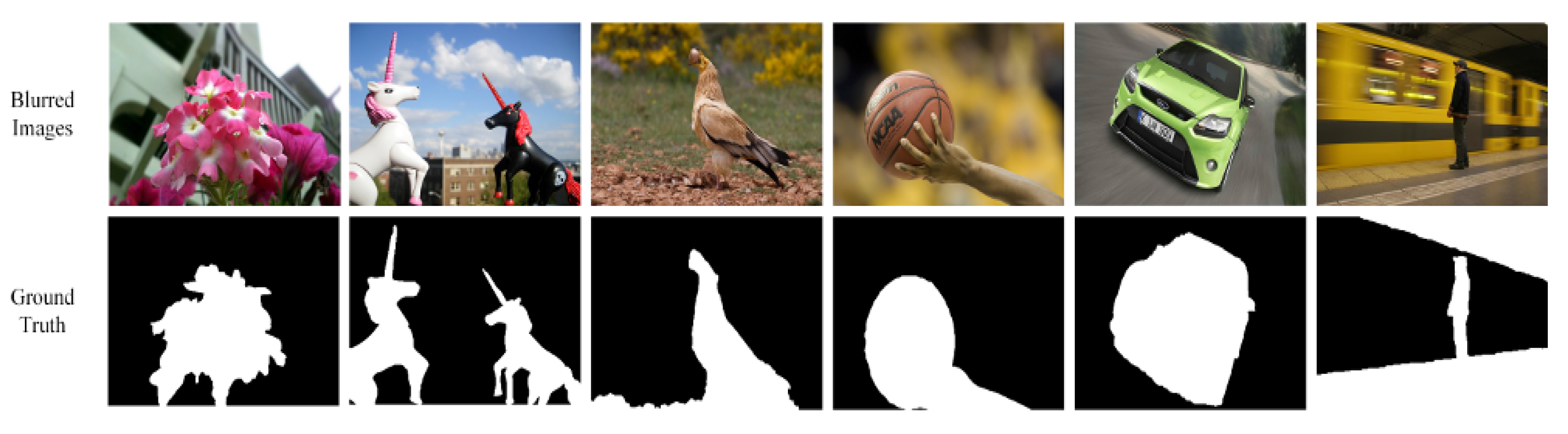
Most of the real-world images are usually affected by the complex and varied nature of the blur. In such cases, blur assessment and segmentation turns out to be a challenging task. Generally, different blur measure operators proposed in the literature are sensitive/receptive to different type of features/characteristics/attributes of the blurred image. Consequently, if the performance of these operators is to be compared, a large dataset is imperative that strives to incorporate broadly varied nature of the blur. Out of the available on-line resources, the dataset of [11] seems an appropriate choice and has been considered in this comprehensive study. This dataset contains 1000 real-world partially blurred images. These are of different resolutions and are collected from the Internet. As humans are the ultimate objects to perceive the images, the human labeled ground-truths are also provided for the blurred and sharp regions. There are 704 images corresponding to defocus blur and 296 images representing the motion blur with different magnitudes of defocus and motion respectively. These images cover various scenarios and comprise of numerous attributes like nature, people, vehicles, man-made structure and other living beings. This dataset provides an ample test-bench to evaluate different blur measures. Few images with ground-truths are shown in Figure 1.
3.2. Methodology
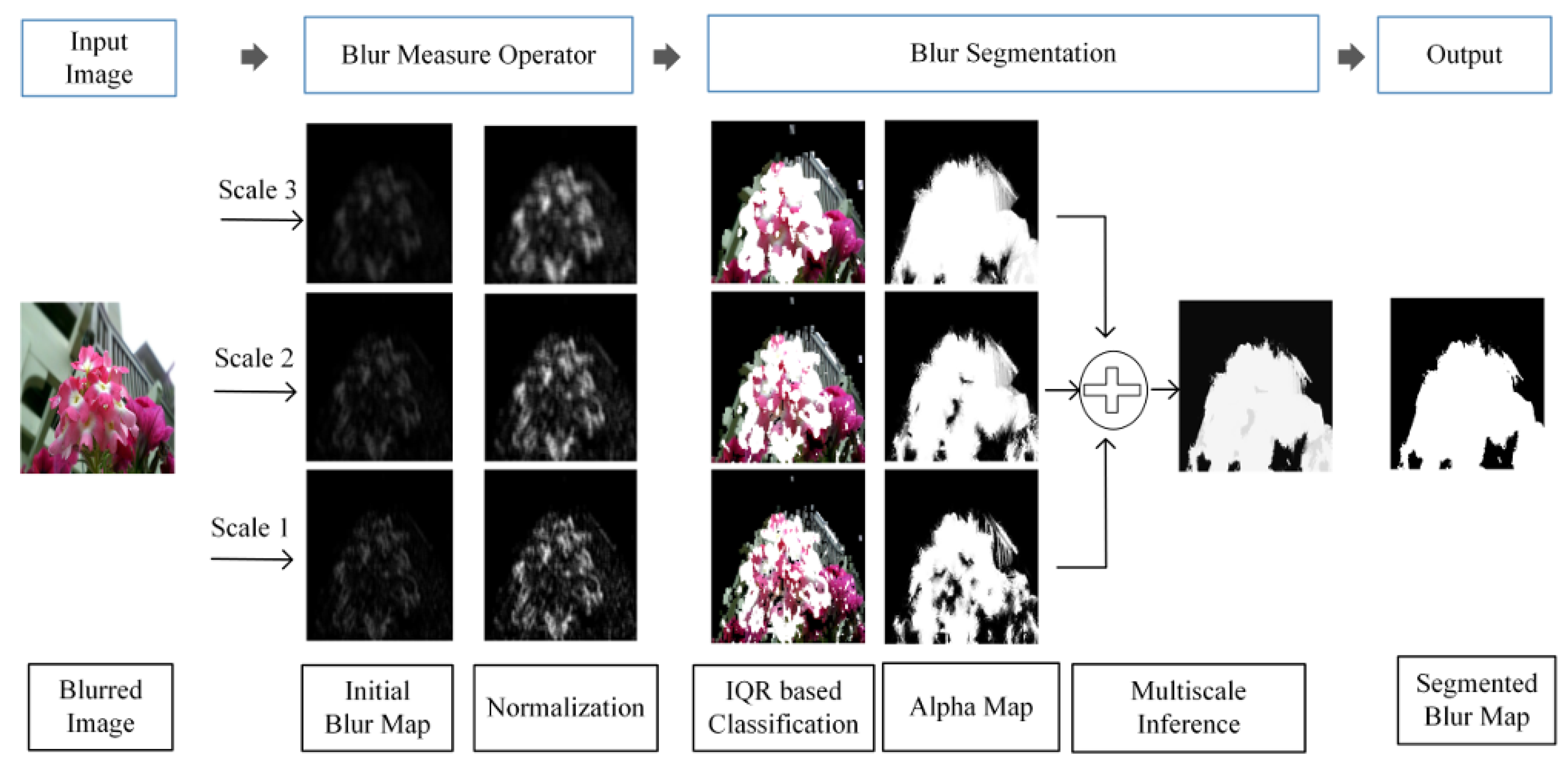
In this section, we present a unified framework for the blur detection and segmentation. The blur measure operators investigated in this study have been mentioned in the next section. We have used the publicly available code of the blur segmentation method originally proposed by Yi and Eramian [14]. However, we have introduced a little modification in the blur map classification step of this framework such that we have employed Interquartile Range (IQR) of the initial blur map for its classification instead of some fixed thresholds. This is more compelling choice and its advantage has been proven by better results. All of the steps of the blur segmentation methodology have been performed at three different scales to account for the varying sizes of the blur as suggested in [11] and followed in [14]. Figure 2 depicts the key steps involved in the blur segmentation process by taking the first image of Figure 1 as an example.
3.2.1. Blur Measures
Let be the blurred input image for which the amount of blurriness is to be computed at each pixel location. This can be achieved by the application of a blur measure operator B in the local neighborhood window-wise environment around a pixel . For this, B is applied on a local image neighborhood window centered at pixel to provide the blur measurement for this pixel. By sliding this neighborhood window for all the image pixels to be at the center of the neighborhood window one-by-one, the whole image can be traversed to result into the generation of the initial blur map .
Then, this initial blur map is normalized linearly so that . The resultant normalized blur map can be expressed as
where and are the minimum and maximum measurements in the initial blur map. In the literature, a wide variety of blur detection techniques and blur measure operators have been proposed to measure the level of blur of either the whole image or neighborhood window or individual pixels. In this work, blur measure operators have been grouped into four broad categories according to their working principle. This categorization is to recognize the similarities and differences, if any, in their performances and then rank them accordingly. A brief description of each of the categories is presented in this section. The interested reader is referred to Appendix A for more detailed description of the blur measure operators which have been analyzed in this work. Abbreviations have been used for the blur measure operators as described in Table 1. This is to refer them conveniently, as well as to signify the category to which they belong.
The four categories of blur measure operators analyzed in this work are:
- Derivative-based operators [DER*]: The blur measure operators in this category are based on the derivative of the image. These operators are based on the assumption that non-blurred images present sharp edges as compared to blurred images. First and second order derivatives of the image neighborhood windows provide the base to distinguish between blurred and non-blurred regions of the image.
- Statistical-based operators [STA*]: The blur measure operators of this category utilize several statistical measures which are computed on image neighborhood windows to differentiate between blurred and non-blurred neighborhood windows in the image.
- Transform-based operators [TRA*]: The blur measure operators within this category are based on the transform domain representations of the image content. These frequency domain representations offer to be the true replica of the same information as in the spatial domain and thus this frequency content of the image can be utilized to differentiate between blurred and non-blurred regions of the image.
- Miscellaneous operators [MIS*]: These operators do not belong to any of the previously mentioned categories.
3.2.2. Blur Classification
The mentioned blur measure operators have been applied on the images of the data set in order to obtain their respective blur maps. After acquiring the initial blur map, pixels need to be declared sharp or blurred, and they need to be separated into blurred and sharp regions respectively. This blur classification phenomenon has been carried out in two steps. In the first step, the initial normalized blur map has been divided into three classes by applying a double threshold , as given by,
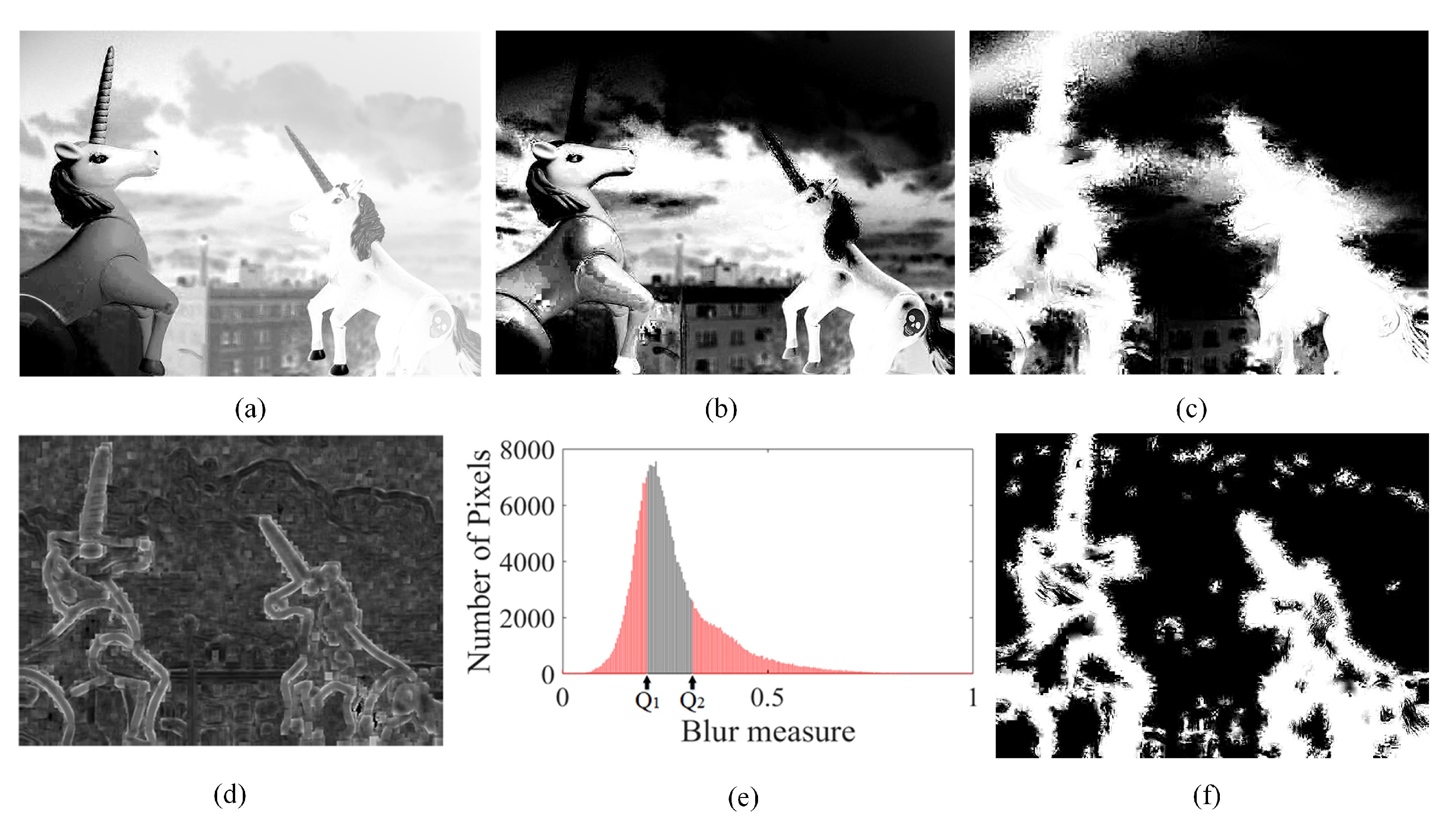
where is the initial alpha map. Authors of [14] have used some fixed precomputed thresholds. However, since different blur measure operators give different blur measures for the same pixels, the classifying thresholds cannot be held fixed to some aprior. In fact, to acknowledge the diversity of each image and each blur measure operator, these thresholds are to be computed adaptively, for each image—operator pair so as to provide uniform and comparable results for the final blur maps. Therefore, we propose to apply thresholds by computing them adaptively. For this, interquartile range (IQR) of the initial normalized blur map of the image has been considered. IQR is a measure of statistical dispersion and variability, and it divides the data into four equal parts. Here, and are taken respectively as the first and third quartiles of the pixel intensity distribution of the image under consideration. By applying this IQR thresholding, pixels in the alpha matting step have been classified initially into three categories: (1) 1 s (2) 0 s and (3) yet to be decided, as expressed in Equation (3). The improved alpha map initialization through IQR can be seen in Figure 3 for the second image of Figure 1.
The pixels which could not have been classified as either 1 or 0 are refined through the optimization in the second step. This refinement of the pixels is achieved through the minimization of the cost function as proposed by [42]
where is the matting Laplacian matrix, is the vectorized alpha map for the pixels in the IQR and is the vectorized alpha map as computed in Equation (3).
3.2.3. Multiscale Inference
Usually, the blurred images have spatially varying blur sizes. In such a case, the consideration of only one size for the local image neighborhood window may not help in inferring about the blurriness accurately [53]. Therefore, three sizes for the local neighborhood window are considered for blur map generation which correspond to three scales, .
Given an input image, the blur measures are computed at three different scales by applying an operator B and then alpha matting is applied at each scale for classification. After acquiring -maps at three different scales, these are fused together using a multi-scale graphical model as proposed by [11]. The total energy on the graphical model is expressed as
where represents the optimized alpha map for a pixel i at a particular scale s and is the alpha map to be inferred. This multi-scale inference makes it feasible to extract small and large sized blur, which makes our methodology more effective. The first data term on the right is the cost of assigning the alpha map values. The second term consists of two parts and it enforces smoothness in the same scale and across different scales. The first part represents the spatial affinity in the four neighbor set for pixel i in the s scale. The second part accounts for the inter-scale affinity. The weight steers the relative importance of these two terms. Equation (5) can be optimized using loopy belief propagation [54].
Finally, the output of the proposed methodology is the gray scale image which is the inferred blur map at the largest scale. However, as the ground truth is in binary (1 and 0), so has also been binarized into 1 and 0 s accordingly by simply applying an adaptive threshold ,
3.3. Evaluation Measures
The relative performance of the blur measure operators can be analyzed quantitatively as they are being tested under the same blur segmentation framework. All of the stated blur measure operators have been applied on the data set for which ground truth depth maps are also available. In this case, ground-truth is our actual observation in which the pixels are clearly labeled as either blurred or sharp. The blur maps are our retrieved results which are obtained by applying blur measure operators, and these can be compared against the ground-truth to provide the relative performance measurements. We have used Precision, recall and F-measure to determine the quality of the retrieved blur maps. Precision is a measure of relevance between the retrieved result and the observation. In our case it refers to the fraction of the detected blurred (sharp) pixels which are actually blurred (sharp) in the ground-truth.
where means that a blurred (sharp) pixel has been correctly detected as blurred (sharp) pixel and expresses that a pixel has been inaccurately detected as blurred (sharp) but it was sharp (blurred) actually.
Recall, also called as sensitivity in binary classification, is a measure of ability to retrieve the relevant results. In our case, it depicts the fraction of the actual blurred (sharp) pixels which are detected.
where means that a pixel has been inaccurately detected as sharp (blurred) but it was blurred (sharp) actually.
Being based on different working principles, different blur measure operators may show different capabilities with respect to precision and recall evaluations. A more suitable measure in this situation is F-measure which takes both precision and recall into consideration. The F-measure computes the accuracy of retrieved result by comparing it with the observation. In our case, segmented blur map is compared with the ground truth. The general form of F-measure is which is based on Van Rijsbergen’s effectiveness measure [55]. It is the weighted harmonic mean of precision and recall such that recall gets times more importance as compared to precision. If the performance objective is to be considered, this allows to place more emphasis on recall or precision [56] as might be required or intended.
These quantitative measures provide an appropriate tool for analysis and evaluation.
4. Results and Discussion
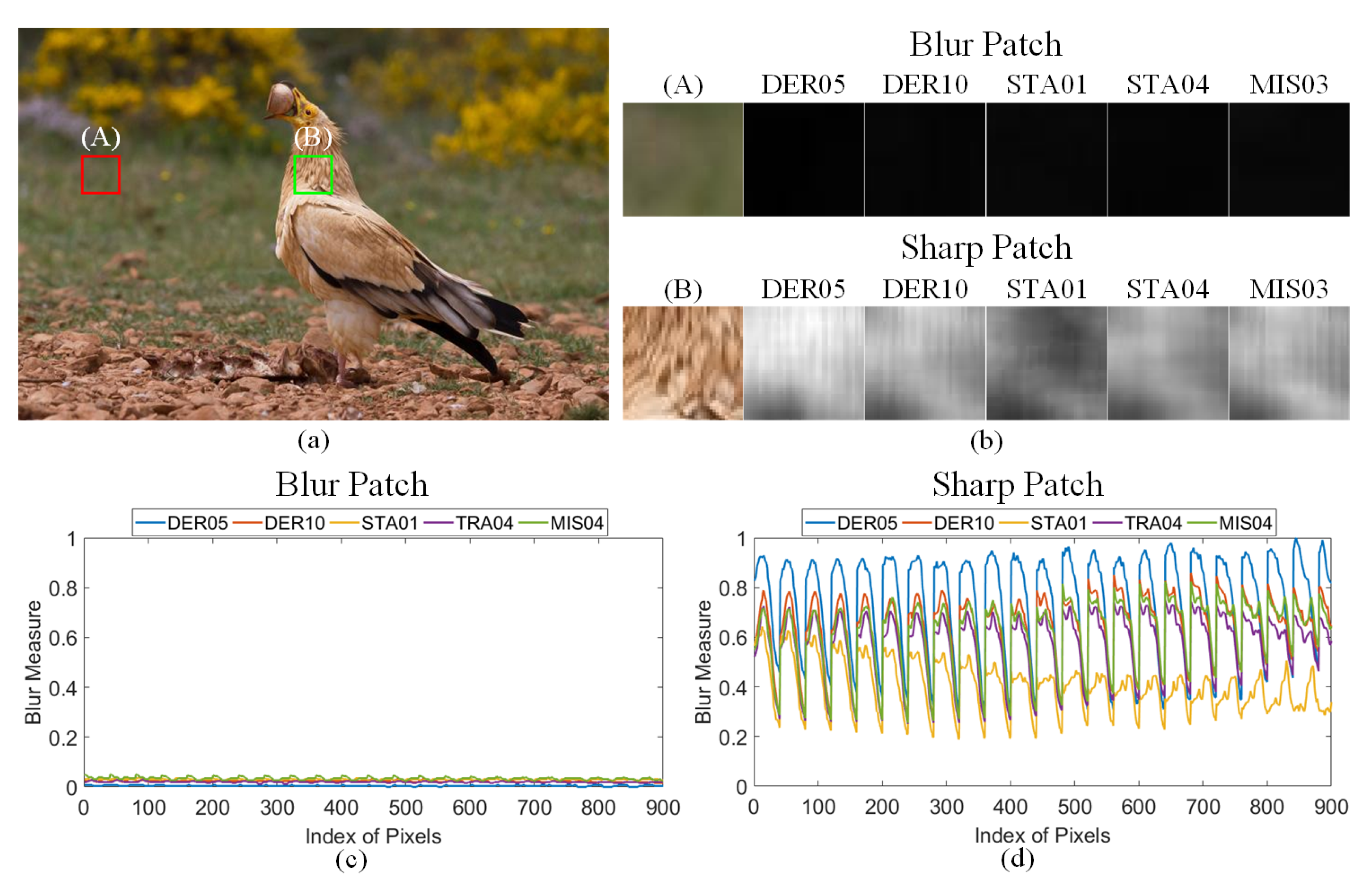
In this section, we describe a number of experiments that have been conducted aiming to analyze the comparative performance of blur measure operators. First of all, we intend to demonstrate that blurred and sharp regions of an image produce clearly distinct responses when a suitable blur measure operator is applied to the image. The essence of a well crafted blur measure operator is that it can help clearly differentiate between blurred and sharp regions. For this objective, two neighborhood windows each of size have been selected as shown in Figure 4a for the third image of Figure 1. The red colored window patch (A) is on the defocused area while the green window patch (B) is placed on the focused region, and these areas have been selected to reveal their potential difference with respect to blur measure operators. Figure 4b displays the image responses when arbitrarily chosen five blur measure operators DER05, DER10, STA01, STA04 and MIS03 have been applied on these selected areas. It clearly indicates that pixels in the blurred area yield small values (black) of blur measures as compared to those of sharp areas. (c) and (d) give the numerical values of blur measurements for the vectorized pixels of the blur and sharp areas, and the marginal gap between them can be clearly identified. More specifically, the blur measures for the pixels in the blurred (defoused) area are less than 0.1 while they all are greater than 0.2 in the case of sharp (focused) area. Moreover, blur measures in the sharp area manifest a lot of fluctuations depicting the high frequency content there.
Regarding the blur detection and segmentation, all of the 32 blur measure operators described in Table 1 have been applied on the randomly selected images of the data set mentioned in Section 3.1. To test each of the blur measure operator under the same framework, the same blur segmentation methodology of Section 3.2 has been followed for all. Even then, the difference in image quality, degree of blur, content and nature of the image can favor some operators. Therefore, the results for images from defocus and motion blur are presented separately. Both qualitative and quantitative results are drawn and shown accordingly. The three scales chosen for local neighborhood patches were , and pixels. The threshold for the binary classification of blur map at the last step of blur segmentation has been taken as the mean of the final blur map, i.e., , where W and H are the dimensions of the final blur map. Firstly, in the qualitative analysis, we present the blur maps obtained by applying the mentioned blur measure operators on the images. These blur maps when compared with the ground-truth give a fair idea about the competency of these operators. In the second case, for quantitative analysis, the evaluation measures mentioned in Section 3.3 have been used to evaluate the relative performance of blur measure operators. A number of experiments have been conducted for this and their results have been presented accordingly. The rankings of the performance of blur measure operators, as learnt through the experiments, are also mentioned for comparative analysis.
4.1. Qualitative Analysis
In this subsection, we conduct two types of experiments and exhibit their results through images. In both type of experiments, we randomly select one image from each of the sets of defocus and motion blurred images as their representative example and apply blur measure operators to retrieve their blur maps.
In the first experiment, we intend to assess the quality of the responses of blur measure operators at the intermediate steps of blur segmentation process. In addition, in order to evaluate the performances relatively, responses of one blur measure operator can be compared with that of another one at all the intermediate steps. For the defocus blur case, the fourth image of Figure 1 has been selected. The responses of blur measure operators for this image have been shown in Figure 5. It can be observed that the performances for DER08 and DER09 are the best while DER02, DER03, STA02, MIS05 and MIS06 are the worst at all the key steps. The highest scale i.e., has been shown for the initial blur and alpha maps.
For the motion blurred case, the fifth image of Figure 1 has been selected and Figure 6 presents its behavior at the steps of segmentation algorithm. It can be noticed that the STA06 produces better results at all the steps while MIS06’s performance is again the worst along with DER01, DER05, DER08 and STA02.
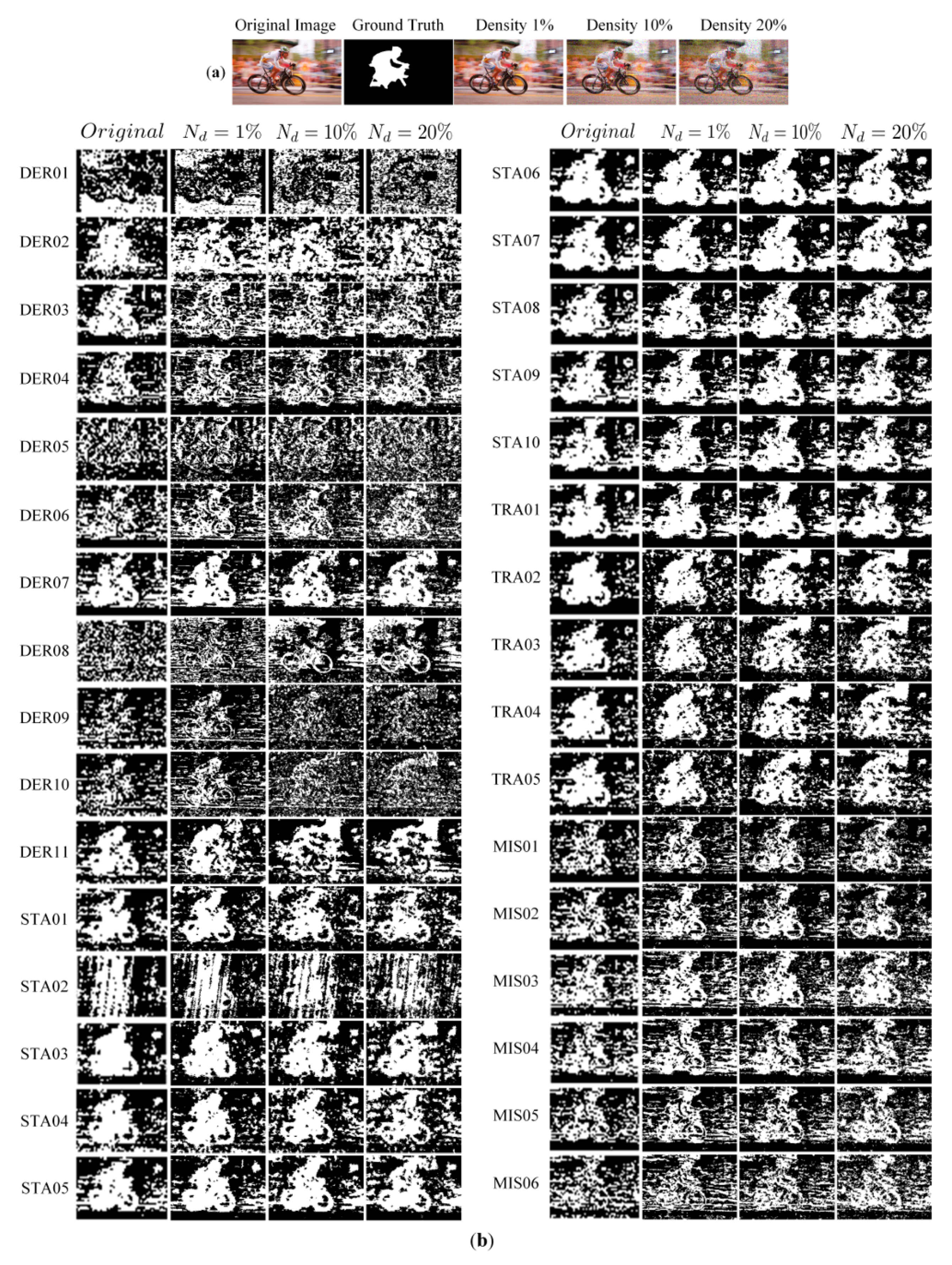
In addition to the blurriness, images in real scenarios may also get corrupted by the noise too. Therefore, to replicate such a common and vulnerable scenario, we conduct the second experiment to explore the effect of noise along with the blur. For this, two types of noise, salt and pepper and random impulse noise have been considered. This constitutes four scenarios: (1) defocus blur with salt and pepper noise, (2) defocus blur with random impulse noise, (3) motion blur with salt and pepper noise, and (4) motion blur with impulse noise. Further, to explore the robustness of blur measure operators against different levels of noise, three density levels , and for both types of noise have been considered. One image from focus blurred and one image from motion blurred image sets has been selected randomly and has been garbled with the noise. The blur maps produced by the blur measure operators for the four scenarios have been shown in Figure 7, Figure 8, Figure 9 and Figure 10, respectively.
For the first case, Figure 7a displays the selected clean image, its ground truth and its three copies corrupted by salt and pepper noise of density , and respectively. In (b), the blur maps obtained by applying blur measure operators have been shown. The best results are manifested by DER09, DER10; while the worst responses are from DER01 and STA02. Not surprisingly, majority of the operators adapted from the autofocus and SFF techniques demonstrated appreciable results, like DER04 to DER11 and STA06. Further, among different categories, transform-based operators show degraded results in case of noise.
4.2. Quantitative Analysis
In the previous subsection, blur measure operators have been described according to their performance when applied on a randomly selected blurred image. However, it does not seem qualified to compare the performance of the blur measure operators on the basis of just a single image. As it is quite possible that the evaluation performances might have been influenced by the particular choice of the image, such that, if some other image might had been selected for analysis, performance ranking of operators might had been different. Therefore, now, we intend to investigate the possibility that whether the ranking of operators is dependent on the choice of the image or not. Put another way, this is to explore the validity of general notion that diverse nature of image content and the type and degree of blur may favor certain type of operators. We select considerable number of images from each of the defocus and motion blurred image sets separately and consider them to be the representative subset of their category. These subsets instead of a single image serve as a better instance to integrate and comprehend the diverse range of image content and level of blurriness. The blur segmentation methodology of Section 3.2 has been applied on these subsets and their results have been compared with their respective ground-truths. The quantitative measures used for the evaluation of performance have been described in Section 3.3. The value of in Equation (9) for the computation of f-measure has been set to be as 0.3. The evaluation measures for all the images in the subset, in both of the defocus and motion blur cases separately, have been combined together to give their average values. These average values are displayed in the bar graphs for the comparison of blur measure operators. The responses of the categories of blur measure operators are also shown in the sub-figures. These category evaluation measures are computed such that the responses of blur measure operators belonging to the same category have been combined together to give the average response for that category.
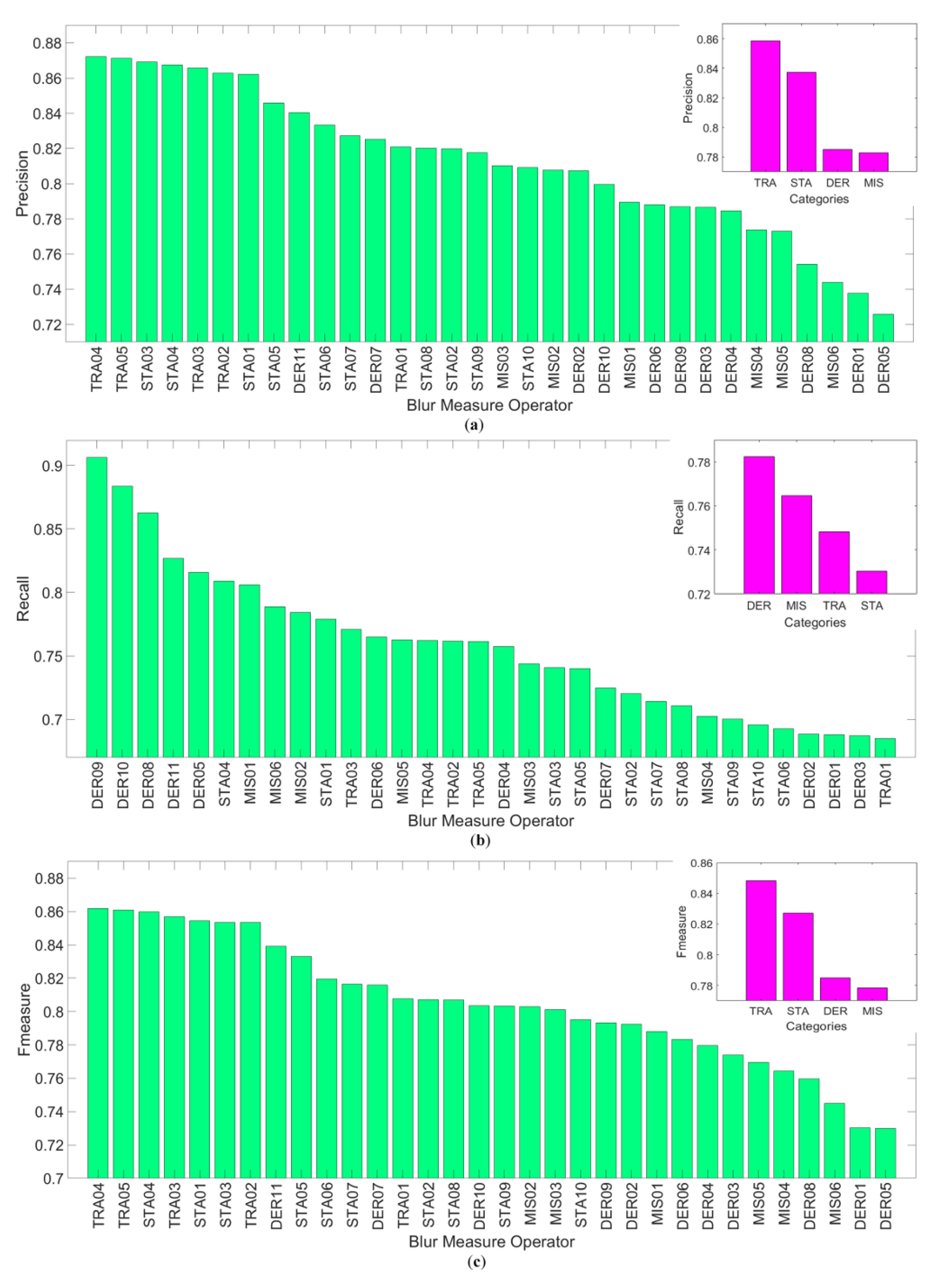
Figure 11 represents the average values of evaluation measures for blur measure operators for the set of 303 images affected by the defocus blur. Highest precision and F-measure are achieved by TRA04 and then TRA05. Those who got highest recall are DER09 and then DER10. Lowest values of precision, and F-measure are attained by DER05 and then DER01.
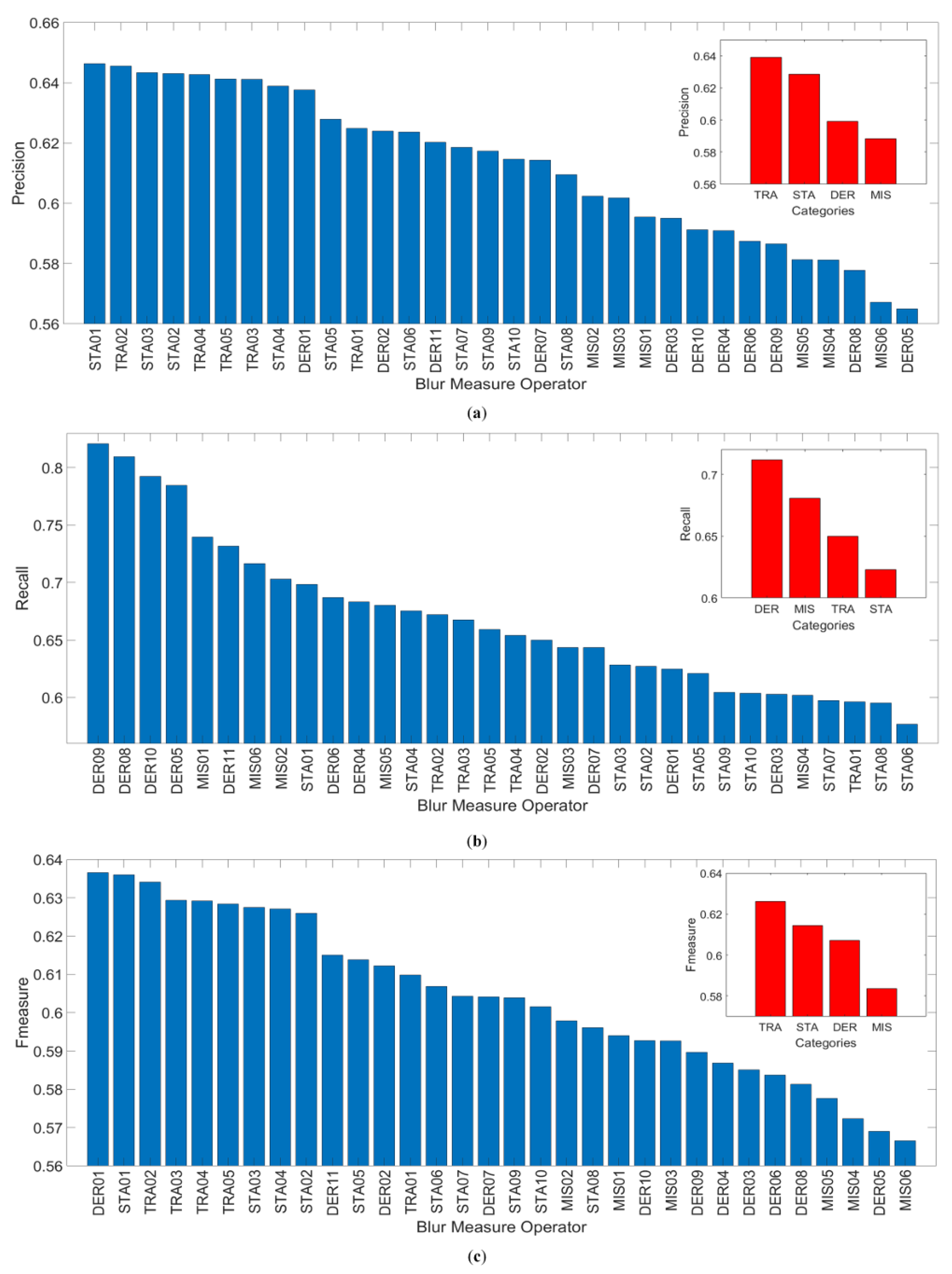
Figure 12 shows the average performance for the 204 defocused blurred images when salt and pepper noise with density is added to them. Highest precision and F-measure are achieved by STA04 and then STA01. Highest recall is for DER09 and then DER08. While the lowest precision, recall and F-measure are exhibited by DER02. While comparing the average responses of categories of blur measure operators in Figure 11 and Figure 12, it reveals that miscellaneous operators show robustness against noise while the derivative-based operators get degraded highly in case of noise.
While, Figure 13 demonstrates the average performance of blur measure operators for the set of 235 images affected by motion blur, Figure 14 shows the average values of evaluation measures for the 296 motion blurred images corrupted by salt and pepper noise of density . It can be seen that STA01 achieves the best results in terms of precision and F-measure, while DER08 is at the top and DER09 is second for recall. The worst values for all three evaluation measures are exhibited by DER02. However, again on average, the best performance is shown by transform-based operators.
In Figure 12 and Figure 14 it can be easily identified that DER02 offers the least robustness against noise.
Hence, it is important to mention that the ranking for the performance of blur measure operators is highly influenced by the choice of the image under consideration. That is, if a different image is selected, the operator which appeared somewhere down in the previous performance ranking may now surface up, even to the top, in the new ranking.
The responses of blur measure operators have been displayed through Figure 11, Figure 12, Figure 13 and Figure 14 for defocus and motion blurred images in clean and noisy scenarios separately. Now, we combine all those results together to have comprehensive evaluation for the performance of all of the blur measure operators. We show average values for all three evaluation measures, precision, recall and f-measure, jointly for the clean and noisy cases in Figure 15 for defocus blur and in Figure 16 for motion blurred images. This is to deduce about the overall response of each of the blur measure operators in defocus and motion blur cases.
5. Conclusions
In this work, we analyze the relative performance of a number of blur measure operators for a single image through the blur segmentation process. A unified framework that treats all of the operators in equal terms has been implemented to compute blur maps and evaluate measures. Few of the studied operators belong to the state-of-the-art blur measure operators proposed in the literature for blur measurement while others have been adopted from the autofocus and shape from focus techniques.
The real world blurred images portray very complex characteristics of blurriness as these images are affected by a number of factors like lens distortion, sensor noise, poor illumination, saturation, nonlinear camera response function and compression in camera pipeline. It has been observed that, on average, STA01, STA03, STA04 and TRA02 to TRA05 exhibit comparatively better results among the blur measure operators considered in this study. It has been noticed that derivative-based operators, like DER08, DER09 and DER10, show highest values for recall. Further, the category of miscellaneous operators show highest robustness against noise, while derivative-based operators show the least robustness, specifically DER02 has been found to offer least robustness. The blur measure operators proposed in the literature and those as discussed in this study seem to be efficient against one or only a few of the factors, but not all; more precisely, they cannot handle all the imperfections in equal terms. However, it has been observed that some operators perform adequately well or worse against almost all imperfections that exist in the real-world images.
Author Contributions
All authors have contributed equally.
Acknowledgments
This work was supported by Basic Science Research Program through the National Research Foundation of Korea (NRF) funded by the Ministry of Education (2016R1D1A1B03933860).
Conflicts of Interest
The authors declare no conflict of interest.
Appendix A. Blur Measure Operators
This appendix summarizes all the blur measure operators which have been investigated in this work. These blur measure operators are applied on the blurred images, , in the local neighborhood window-wise environment by taking each pixel at the center of the neighborhood window . By sliding this neighborhood window to have all image pixels at its central position, one-by-one, the whole image is traversed to provide the blur measures for all the pixels.
Appendix A.1. Derivative-Based Operators
Gradient Histogram Span
The gradient magnitude of sharp images tends to be heavy-tailed distribution than a Gaussian distribution [11,17,57], and thus it can be modeled by a Gaussian mixture model (GMM) of two components given by: , where and are the relative weights of Gaussian components, and are the mean with value , and are the standard deviations with , and is the image gradient magnitude at pixel . The blur measure is:
Kurtosis
The blur measure by computing kurtosis [11] is given by
where is kurtosis such that is the expectation operator for input data vector a with mean , and , are the gradients of I in x and y-directions, respectively.
Gaussian Derivative
The first order Gaussian derivative as used in autofocusing [58] can also be used for blur calculation
where ⊗ is the convolution operator, and and are the partial derivatives of Gaussian function in the x and y-directions, respectively.
Gradient Energy
The sum of squares of first partial derivatives in the x and y-directions has been used as focus measure [59] and can also by used for blur measurement
where and .
Squared Gradient
As [60] proposed it to be the image quality, the square of the image gradient in only one direction (horizontal) can also be considered as the blur measure for a pixel (x,y) in a neighborhood window
Tenengrad
The well-celebrated focus measure based on image gradients obtained by convolving the image with the Sobel operator [61] can be used as a blur measure
where and are the image gradients in x and y-directions.
Tenengrad Variance
The variance of the image gradient magnitudes as used in [61] can be used as blur measure
where represents the gradient magnitude at pixel location such that and are the image gradients obtained by convolving the image with the Sobel operator in x and y-directions, respectively. is the mean of gradient magnitudes in the neighborhood window and it is given by .
Energy of Laplacian
The energy of the second derivatives in a local neighborhood window of the image measures the sharpness for the central pixel [59]
where is the image Laplacian obtained by convolving I with the Laplacian mask.
Modified Laplacian
By taking the absolute values of the second derivatives in x and y directions, the focus measure proposed by [62] can be computed as
where is the modified Laplacian of I and ⊗ is the convolution operator.
Diagonal Modified Laplacian
The diagonal pixels can also be included in Laplacian mask by acknowledging their longer distances [63]
where .
Variance of Laplacian
The variance of image Laplacian as a focus measure in autofocus [61] can be considered as blur measure for central pixel in
where is the mean value of image Laplacian in .
Appendix A.2. Statistical-Based Operators
Singular Value Decomposition
This blur measure is based on the eigen-values which are computed for each pixel in the image by placing that pixel in the center of a small image neighborhood window . Su et al. [16] utilized singular value decomposition of an image neighborhood window as a blur measure by exploiting the fact that larger singular values correspond to the the overall look of the neighborhood window while smaller singular values represent fine details. The proposed blur measure is
where k largest eigen-values have been considered.
Sparsity of Dark Channel
Pan et al. [64] enforces the sparsity of dark channel to deblur an image I. The dark channel for a pixel in a neighborhood window is defined as
where is the c-th color channel.
Total Variation
By measuring the diversity in intensity values of image pixels in a small neighborhood, the blur can be estimated for that patch. Ref. [65] suggested such a measure:
where is the total variation of smaller blocks (let is of ) in the image neighborhood window .
Local Binary Pattern
Yi et al. [14] exploits the observation that local neighborhood windows in blurry regions, in comparison with the sharp regions, have significantly lesser amount of higher LBPs (6 to 9 in case of 8-bit LBP), and proposed a blur measure given by
where is the number of rotation-invariant uniform 8-bit LBP pattern of type i, and N is the total number of pixels in the image neighborhood window.
Gray-Level Variance
The variance of the image gray-levels as used in autofocus [66] can be taken as the blur measure for the central pixel in a local window
where is the mean gray-level of pixels in the neighborhood window .
Gray-Level Local Variance
The local variance of gray-levels has been proposed as a focus measure [61] and it can be reformulated as a blur measure
where and are the variance and mean value within
Normalized Gray-Level Variance
The image sharpness and blurriness can be differentiate by the normalized gray-level variance [67]
where is the mean value for computed over the neighborhood window .
Histogram Entropy
Entropy and range of the histogram [66] of the image indicate the diversity of information and can be utilized as the sharpness measure
where is the frequency of the k-th gray-level within .
DCT Energy Ratio
Shen and Chen [68] used the DC/AC ratio of discrete cosine transform (DCT) for focus measure and it can be used as the blur measure
where is the DCT in an sub-block.
DCT Reduced Energy Ratio
Lee et al. [69] suggested an improvement that 5 out of 63 AC coefficients of DCT can be used for focus measure and it can be used as blur measure
Appendix A.3. Transform-Based Operators
Power Spectrum
In the power spectrum of a blurred image, in contrast to sharp image, high frequency components posses lesser energy as compared to the energy of low frequency components. Thus, a blurred image has its average power located at a lower frequency , and [1] utilized it as a measure:
where is the squared magnitude of DFT of image neighborhood window in polar coordinates and n is the number of quantizations of .
High-Frequency Multiscale Fusion and Sort Transform
By taking various sized neighborhood windows around a central pixel, Golestaneh et al. [31] computes high frequency DCT coefficients of gradient magnitudes, groups them in a number of layers after sorting and then normalizes them between [0, 1]. The blur measure for a pixel p is given by
where represents its tth DCT coefficient which has been normalized among the tth DCT coefficients of all image pixels, and represents the size of a square neighborhood window.
Sum of Wavelet Coefficients
In the first level of discrete wavelet transform (DWT), the image is decomposed into four sub images such as , , and representing the three detail sub bands and one coarse sub band, respectively. Iteratively, coarse sub band is further divided into three detail sub bands and one coarse sub band. Yang and Nelson [70] combined the sub-bands to propose a focus operator which can be treated as a blur measure and is given by
where is the corresponding window of in DWT sub bands.
Variance of Wavelet Coefficients
The variance of wavelet coefficients within for focus measurement as proposed in [70] can also be used as blur measure
where , and are the mean value of the respective sub bands within .
Ratio of Wavelet Coefficients
Xie et al.’s operator [71] that involves the high and low frequency coefficients, can be used as the blur measure
where and and k represents the k-th level wavelet.
Appendix A.4. Miscellaneous Operators
Brenner’s Operator
A blur measure for a pixel can be derived from Brenner [67] by taking horizontal and vertical squared second differences of gray-levels in an image neighborhood window
Image Contrast
Nanda et al.’s operator [72] can be used as a blur measure by calculating image contrast for a pixel in a local neighborhood window as given by
where is the image contrast for pixel .
Image Curvature
Helmli and Scherer [73] interpolated the gray-levels of the image through a quadratic surface. The curvature of this surface can be used as a blur measure
where ’s are the coefficients of the surface.
Steerable Filters-Based Measure
The filtered image obtained by applying steerable filters [74] on the image can be considered for the blur map estimation
where is the maximum response out of the N responses obtained by applying filters.
Spatial Frequency
The operator of [75] can be considered as the blur measure
where and are the derivatives of the image in x and y directions respectively.
Vollath’s Autocorrelation
Image autocorrelation-based operator proposed by [67] for auto-focusing can be utilized for blur measurement
References
- Liu, R.; Li, Z.; Jia, J. Image partial blur detection and classification. In Proceedings of the IEEE Conference on Computer Vision and Pattern Recognition (CVPR 2008), Anchorage, AK, USA, 24–26 June 2008; pp. 1–8. [Google Scholar]
- Jiang, P.; Ling, H.; Yu, J.; Peng, J. Salient region detection by ufo: Uniqueness, focusness and objectness. In Proceedings of the IEEE International Conference on Computer Vision, Sydney, Australia, 1–8 December 2013; pp. 1976–1983. [Google Scholar]
- Derpanis, K.G.; Lecce, M.; Daniilidis, K.; Wildes, R.P. Dynamic scene understanding: The role of orientation features in space and time in scene classification. In Proceedings of the 2012 IEEE Conference on Computer Vision and Pattern Recognition (CVPR), Providence, RI, USA, 16–21 June 2012; pp. 1306–1313. [Google Scholar]
- Bahrami, K.; Kot, A.C.; Fan, J. A novel approach for partial blur detection and segmentation. In Proceedings of the 2013 IEEE International Conference on Multimedia and Expo (ICME), San Jose, CA, USA, 15–19 July 2013; pp. 1–6. [Google Scholar]
- Bae, S.; Durand, F. Defocus magnification. In Computer Graphics Forum; Wiley Online Library: Hoboken, NJ, USA, 2007; Volume 26, pp. 571–579. [Google Scholar]
- Dandres, L.; Salvador, J.; Kochale, A.; Susstrunk, S. Non parametric blur map regression for depth of field extension. IEEE Trans. Image Process. 2016, 25, 1660–1673. [Google Scholar] [CrossRef] [PubMed]
- Lin, J.; Ji, X.; Xu, W.; Dai, Q. Absolute depth estimation froma single defocused image. IEEE Trans. Image Process. 2013, 22, 4545–4550. [Google Scholar] [PubMed]
- Tang, C.; Hou, C.; Song, Z. Defocus map estimation from a single image via spectrum contrast. Opt. Lett. 2013, 38, 1706–1708. [Google Scholar] [CrossRef] [PubMed]
- Chen, D.J.; Chen, H.T.; Chang, L.W. Fast defocus map estimation. In Proceedings of the 2016 IEEE International Conference on Image Processing (ICIP), Phoenix, AZ, USA, 25–28 September 2016; pp. 3962–3966. [Google Scholar]
- Gast, J.; Sellent, A.; Roth, S. Parametric Object Motion from Blur. In Proceedings of the IEEE Conference on Computer Vision and Pattern Recognition, Las Vegas, NV, USA, 26 June–1 July 2016; pp. 1846–1854. [Google Scholar]
- Shi, J.; Xu, L.; Jia, J. Discriminative blur detection features. In Proceedings of the 2014 IEEE Conference on Computer Vision and Pattern Recognition, Columbus, OH, USA, 23–28 June 2014; pp. 2965–2972. [Google Scholar]
- Shi, J.; Xu, L.; Jia, J. Just noticeable defocus blur detection and estimation. In Proceedings of the 2015 IEEE Conference on Computer Vision and Pattern Recognition, Boston, MA, USA, 7–12 June 2015; pp. 657–665. [Google Scholar]
- Tang, C.; Wu, J.; Hou, Y.; Wang, P.; Li, W. A Spectral and Spatial Approach of Coarse-to-Fine Blurred Image Region Detection. IEEE Signal Process. Lett. 2016, 23, 1652–1656. [Google Scholar] [CrossRef]
- Yi, X.; Eramian, M. LBP-based segmentation of defocus blur. IEEE Trans. Image Process. 2016, 25, 1626–1638. [Google Scholar] [CrossRef] [PubMed]
- Zhu, T.; Karam, L.J. Efficient perceptual-based spatially varying out-of-focus blur detection. In Proceedings of the 2016 IEEE International Conference on Image Processing (ICIP), Phoenix, AZ, USA, 25–28 September 2016; pp. 2673–2677. [Google Scholar]
- Su, B.; Lu, S.; Tan, C.L. Blurred image region detection and classification. In Proceedings of the 19th ACM International Conference on Multimedia, Scottsdale, AZ, USA, 28 November–1 December 2011; pp. 1397–1400. [Google Scholar]
- Zhao, J.; Feng, H.; Xu, Z.; Li, Q.; Tao, X. Automatic blur region segmentation approach using image matting. Signal Image Video Process. 2013, 7, 1173–1181. [Google Scholar] [CrossRef]
- Lai, W.S.; Huang, J.B.; Hu, Z.; Ahuja, N.; Yang, M.H. A comparative study for single image blind deblurring. In Proceedings of the 2016 IEEE Conference on Computer Vision and Pattern Recognition, Las Vegas, NV, USA, 27–30 June 2016; pp. 1701–1709. [Google Scholar]
- Pertuz, S.; Puig, D.; Garcia, M.A. Analysis of focus measure operators for shape-from-focus. Pattern Recognit. 2013, 46, 1415–1432. [Google Scholar] [CrossRef]
- Wang, J.Z.; Li, J.; Gray, R.M.; Wiederhold, G. Unsupervised multiresolution segmentation for images with low depth of field. IEEE Trans. Pattern Anal. Mach. Intell. 2001, 23, 85–90. [Google Scholar] [CrossRef]
- Zhou, C.; Cossairt, O.; Nayar, S. Depth from diffusion. In Proceedings of the 2010 IEEE Conference on Computer Vision and Pattern Recognition (CVPR), San Francisco, CA, USA, 13–18 June 2010; pp. 1110–1117. [Google Scholar]
- Elder, J.H.; Zucker, S.W. Local scale control for edge detection and blur estimation. IEEE Trans. Pattern Anal. Mach. Intell. 1998, 20, 699–716. [Google Scholar] [CrossRef]
- Namboodiri, V.P.; Chaudhuri, S. Recovery of relative depth from a single observation using an uncalibrated (real-aperture) camera. In Proceedings of the IEEE Conference on Computer Vision and Pattern Recognition (CVPR 2008), Anchorage, AK, USA, 23–28 June 2008; pp. 1–6. [Google Scholar]
- Tai, Y.W.; Brown, M.S. Single image defocus map estimation using local contrast prior. In Proceedings of the 2009 16th IEEE International Conference on Image Processing (ICIP), Cairo, Egypt, 7–12 November 2009; pp. 1797–1800. [Google Scholar]
- Zhuo, S.; Sim, T. Defocus map estimation from a single image. Pattern Recognit. 2011, 44, 1852–1858. [Google Scholar] [CrossRef]
- Peng, Y.T.; Zhao, X.; Cosman, P.C. Single underwater image enhancement using depth estimation based on blurriness. In Proceedings of the 2015 IEEE International Conference on Image Processing (ICIP), Quebec City, QC, Canada, 27–30 September 2015; pp. 4952–4956. [Google Scholar]
- Zhang, Y.; Hirakawa, K. Blur processing using double discrete wavelet transform. In Proceedings of the 2013 IEEE Conference on Computer Vision and Pattern Recognition, Portland, OR, USA, 23–28 June 2013; pp. 1091–1098. [Google Scholar]
- Zhu, X.; Cohen, S.; Schiller, S.; Milanfar, P. Estimating spatially varying defocus blur from a single image. IEEE Trans. Image Process. 2013, 22, 4879–4891. [Google Scholar] [CrossRef] [PubMed]
- Lin, H.T.; Tai, Y.W.; Brown, M.S. Motion regularization for matting motion blurred objects. IEEE Trans. Pattern Anal. Mach. Intell. 2011, 33, 2329–2336. [Google Scholar] [PubMed]
- Oliveira, J.P.; Figueiredo, M.A.; Bioucas-Dias, J.M. Parametric blur estimation for blind restoration of natural images: Linear motion and out-of-focus. IEEE Trans. Image Process. 2014, 23, 466–477. [Google Scholar] [CrossRef] [PubMed]
- Golestaneh, S.A.; Karam, L.J. Spatially-Varying Blur Detection Based on Multiscale Fused and Sorted Transform Coefficients of Gradient Magnitudes. arXiv, 2017; arXiv:1703.07478. [Google Scholar]
- Chakrabarti, A.; Zickler, T.; Freeman, W.T. Analyzing spatially-varying blur. In Proceedings of the 2010 IEEE Conference on Computer Vision and Pattern Recognition (CVPR), San Francisco, CA, USA, 13–18 June 2010; pp. 2512–2519. [Google Scholar]
- Pan, J.; Hu, Z.; Su, Z.; Lee, H.Y.; Yang, M.H. Soft-segmentation guided object motion deblurring. In Proceedings of the 2016 IEEE Conference on Computer Vision and Pattern Recognition, Las Vegas, NV, USA, 26 June–1 July 2016; pp. 459–468. [Google Scholar]
- Hyun Kim, T.; Ahn, B.; Mu Lee, K. Dynamic scene deblurring. In Proceedings of the 2013 IEEE International Conference on Computer Vision, Sydney, Australia, 1–8 December 2013; pp. 3160–3167. [Google Scholar]
- Whyte, O.; Sivic, J.; Zisserman, A.; Ponce, J. Non-uniform deblurring for shaken images. Int. J. Comput. Vis. 2012, 98, 168–186. [Google Scholar] [CrossRef]
- Gupta, A.; Joshi, N.; Zitnick, C.L.; Cohen, M.; Curless, B. Single image deblurring using motion density functions. In Proceedings of the European Conference on Computer Vision, Heraklion, Greece, 5–11 September 2010; pp. 171–184. [Google Scholar]
- Hirsch, M.; Schuler, C.J.; Harmeling, S.; Schölkopf, B. Fast removal of non-uniform camera shake. In Proceedings of the 2011 IEEE International Conference on Computer Vision, Barcelona, Spain, 6–13 November 2011; pp. 463–470. [Google Scholar]
- Shan, Q.; Xiong, W.; Jia, J. Rotational motion deblurring of a rigid object from a single image. In Proceedings of the IEEE 11th International Conference on Computer Vision (ICCV 2007), Rio de Janeiro, Brazil, 14–20 October 2007; pp. 1–8. [Google Scholar]
- Tai, Y.W.; Tan, P.; Brown, M.S. Richardson-Lucy deblurring for scenes under a projective motion path. IEEE Trans. Pattern Anal. Mach. Intell. 2011, 33, 1603–1618. [Google Scholar] [PubMed]
- Raskar, R.; Agrawal, A.; Tumblin, J. Coded exposure photography: motion deblurring using fluttered shutter. ACM Trans. Graph. 2006, 25, 795–804. [Google Scholar] [CrossRef]
- Tai, Y.W.; Du, H.; Brown, M.S.; Lin, S. Correction of spatially varying image and video motion blur using a hybrid camera. IEEE Trans. Pattern Anal. Mach. Intell. 2010, 32, 1012–1028. [Google Scholar] [PubMed]
- Levin, A.; Lischinski, D.; Weiss, Y. A closed-form solution to natural image matting. IEEE Trans. Pattern Anal. Mach. Intell. 2008, 30, 228–242. [Google Scholar] [CrossRef] [PubMed]
- Dai, S.; Wu, Y. Removing partial blur in a single image. In Proceedings of the IEEE Conference on Computer Vision and Pattern Recognition (CVPR 2009), Miami, FL, USA, 20–25 June 2009; pp. 2544–2551. [Google Scholar]
- Tai, Y.W.; Kong, N.; Lin, S.; Shin, S.Y. Coded exposure imaging for projective motion deblurring. In Proceedings of the 2010 IEEE Conference on Computer Vision and Pattern Recognition (CVPR), San Francisco, CA, USA, 13–18 June 2010; pp. 2408–2415. [Google Scholar]
- Pan, J.; Hu, Z.; Su, Z.; Yang, M.H. Deblurring text images via L0-regularized intensity and gradient prior. In Proceedings of the 2014 IEEE Conference on Computer Vision and Pattern Recognition, Columbus, OH, USA, 23–28 June 2014; pp. 2901–2908. [Google Scholar]
- Xu, L.; Jia, J. Two-phase kernel estimation for robust motion deblurring. In European Conference on Computer Vision; Springer: Berlin, Germeny, 2010; pp. 157–170. [Google Scholar]
- Fattal, R.; Goldstein, A. Blur-Kernel Estimation From Spectral Irregularities. U.S. Patent 9,008,453, 14 April 2015. [Google Scholar]
- Hu, Z.; Yang, M.H. Good regions to deblur. In Proceedings of the Computer Vision–ECCV 2012, Florence, Italy, 7–13 October 2012; pp. 59–72. [Google Scholar]
- Zhu, X.; Šroubek, F.; Milanfar, P. Deconvolving PSFs for a better motion deblurring using multiple images. In Proceedings of the Computer Vision–ECCV 2012, Florence, Italy, 7–13 October 2012; pp. 636–647. [Google Scholar]
- Levin, A.; Fergus, R.; Durand, F.; Freeman, W.T. Image and depth from a conventional camera with a coded aperture. ACM Trans. Graph. 2007, 26, 70. [Google Scholar] [CrossRef]
- Cheong, H.; Chae, E.; Lee, E.; Jo, G.; Paik, J. Fast image restoration for spatially varying defocus blur of imaging sensor. Sensors 2015, 15, 880–898. [Google Scholar] [CrossRef] [PubMed]
- Chan, S.H.; Nguyen, T.Q. Single image spatially variant out-of-focus blur removal. In Proceedings of the 18th IEEE International Conference on Image Processing (ICIP), Brussels, Belgium, 11–14 September 2011; pp. 677–680. [Google Scholar]
- Yan, Q.; Xu, L.; Shi, J.; Jia, J. Hierarchical saliency detection. In Proceedings of the IEEE Conference on Computer Vision and Pattern Recognition, Portland, OR, USA, 23–28 June 2013; pp. 1155–1162. [Google Scholar]
- Murphy, K.P.; Weiss, Y.; Jordan, M.I. Loopy belief propagation for approximate inference: An empirical study. In Proceedings of the Fifteenth Conference on Uncertainty in Artificial Intelligence, Stockholm, Sweden, 30 July–1 August 1999; Morgan Kaufmann Publishers Inc.: Burlington, MA, USA, 1999; pp. 467–475. [Google Scholar]
- Van Rijsbergen, C. Information Retrieval. Dept. of Computer Science, University of Glasgow, 1979. Available online: citeseer.ist.psu.edu/vanrijsbergen79information.html (accessed on 17 May 2018).
- Li, X.; Wang, Y.Y.; Acero, A. Learning query intent from regularized click graphs. In Proceedings of the 31st Annual International ACM SIGIR Conference on Research and Development in Information Retrieval, Singapore, 20–24 July 2008; pp. 339–346. [Google Scholar]
- Takayama, N.; Takahashi, H. Blur map generation based on local natural image statistics for partial blur segmentation. IEICE Trans. Inf. Syst. 2017, 100, 2984–2992. [Google Scholar] [CrossRef]
- Geusebroek, J.M.; Cornelissen, F.; Smeulders, A.W.; Geerts, H. Robust autofocusing in microscopy. Cytom. Part A 2000, 39, 1–9. [Google Scholar] [CrossRef]
- Subbarao, M.; Choi, T.S.; Nikzad, A. Focusing techniques. Opt. Eng. 1993, 32, 2824–2836. [Google Scholar] [CrossRef]
- Eskicioglu, A.M.; Fisher, P.S. Image quality measures and their performance. IEEE Trans. Commun. 1995, 43, 2959–2965. [Google Scholar] [CrossRef]
- Pech-Pacheco, J.L.; Cristóbal, G.; Chamorro-Martinez, J.; Fernández-Valdivia, J. Diatom autofocusing in brightfield microscopy: A comparative study. In Proceedings of the 15th International Conference on Pattern Recognition, Barcelona, Spain, 3–7 September 2000; Volume 3, pp. 314–317. [Google Scholar]
- Nayar, S.K.; Nakagawa, Y. Shape from focus. IEEE Trans. Pattern Anal. Mach. Intell. 1994, 16, 824–831. [Google Scholar] [CrossRef]
- Thelen, A.; Frey, S.; Hirsch, S.; Hering, P. Improvements in shape-from-focus for holographic reconstructions with regard to focus operators, neighborhood-size, and height value interpolation. IEEE Trans. Image Process. 2009, 18, 151–157. [Google Scholar] [CrossRef] [PubMed]
- Pan, J.; Sun, D.; Pfister, H.; Yang, M.H. Blind image deblurring using dark channel prior. In Proceedings of the IEEE Conference on Computer Vision and Pattern Recognition, Las Vegas, NV, USA, 26 June–1 July 2016; pp. 1628–1636. [Google Scholar]
- Vu, C.T.; Phan, T.D.; Chandler, D.M. A Spectral and Spatial Measure of Local Perceived Sharpness in Natural Images. IEEE Trans. Image Process. 2012, 21, 934–945. [Google Scholar] [CrossRef] [PubMed]
- Krotkov, E.; Martin, J.P. Range from focus. In Proceedings of the 1986 IEEE International Conference on Robotics and Automation, San Francisco, CA, USA, 7–10 April 1986; Volume 3, pp. 1093–1098. [Google Scholar]
- Santos, A.; Ortiz de Solórzano, C.; Vaquero, J.J.; Pena, J.; Malpica, N.; Del Pozo, F. Evaluation of autofocus functions in molecular cytogenetic analysis. J. Microsc. 1997, 188, 264–272. [Google Scholar] [CrossRef] [PubMed] [Green Version]
- Shen, C.H.; Chen, H.H. Robust focus measure for low-contrast images. In Proceedings of the International Conference on Consumer Electronics (ICCE’06), Las Vegas, NV, USA, 7–11 January 2006; pp. 69–70. [Google Scholar]
- Lee, S.Y.; Yoo, J.T.; Kumar, Y.; Kim, S.W. Reduced energy-ratio measure for robust autofocusing in digital camera. IEEE Signal Process. Lett. 2009, 16, 133–136. [Google Scholar] [CrossRef]
- Yang, G.; Nelson, B.J. Wavelet-based autofocusing and unsupervised segmentation of microscopic images. In Proceedings of the IEEE/RSJ International Conference on Intelligent Robots and Systems (IROS 2003), Las Vegas, NV, USA, 27–31 October 2003; Volume 3, pp. 2143–2148. [Google Scholar]
- Xie, H.; Rong, W.; Sun, L. Wavelet-based focus measure and 3-d surface reconstruction method for microscopy images. In Proceedings of the 2006 IEEE/RSJ International Conference on Intelligent Robots and Systems, Beijing, China, 9–15 October 2006; pp. 229–234. [Google Scholar]
- Nanda, H.; Cutler, R. Practical Calibrations for a Real-Time Digital Omnidirectional Camera. 2001. CVPR Technical Sketch. Available online: https://www.researchgate.net/publication/228952354_Practical_calibrations_for_a_real-time_digital_omnidirectional_camera (accessed on 17 May 2018).
- Helmli, F.S.; Scherer, S. Adaptive shape from focus with an error estimation in light microscopy. In Proceedings of the 2nd International Symposium on Image and Signal Processing and Analysis (ISPA 2001), Pula, Croatia, 19–21 June 2001; pp. 188–193. [Google Scholar]
- Minhas, R.; Mohammed, A.A.; Wu, Q.J.; Sid-Ahmed, M.A. 3D shape from focus and depth map computation using steerable filters. In Proceedings of the International Conference Image Analysis and Recognition, Halifax, NC, Canada, 6–8 July 2009; pp. 573–583. [Google Scholar]
- Huang, W.; Jing, Z. Evaluation of focus measures in multi-focus image fusion. Pattern Recognit. Lett. 2007, 28, 493–500. [Google Scholar] [CrossRef]
Figure 1.
Sample images and their ground-truth from the data set. Row 1: First 4 images are defocus blurred while last 2 images are motion blurred. Row 2 displays ground-truth blur maps for row 1 images.
Figure 1.
Sample images and their ground-truth from the data set. Row 1: First 4 images are defocus blurred while last 2 images are motion blurred. Row 2 displays ground-truth blur maps for row 1 images.

Figure 2.
Framework for Blur Segmentation.

Figure 3.
Comparison for the setting of thresholds in the alpha matting step either by some predefined fixed values or computing them adaptively through interquartile range (IQR). Initial alpha maps are obtained by applying Kurtosis in a neighborhood window of size pixels. First row shows the initial alpha maps computed by taking the randomly selected thresholds (a) , (b) and (c) . (d) represents the normalized initial blur map of the input image. (e) IQR for the histogram of (d) where and . (f) Initial alpha map by setting as in Equation (3).

Figure 4.
Blur measure operators’ responses for the blurred and sharp areas. (a) One neighborhood window selected for the blurred and sharp areas each. (b) Imagery responses of the neighborhood windows for five blur measure operators. (c,d) Display the blur measures for vectorized pixels in case of blur and sharp window patches respectively.

Figure 5.
Successive stages of segmentation process for a defocus blurred image.

Figure 6.
Successive stages of segmentation process for a motion blurred image.
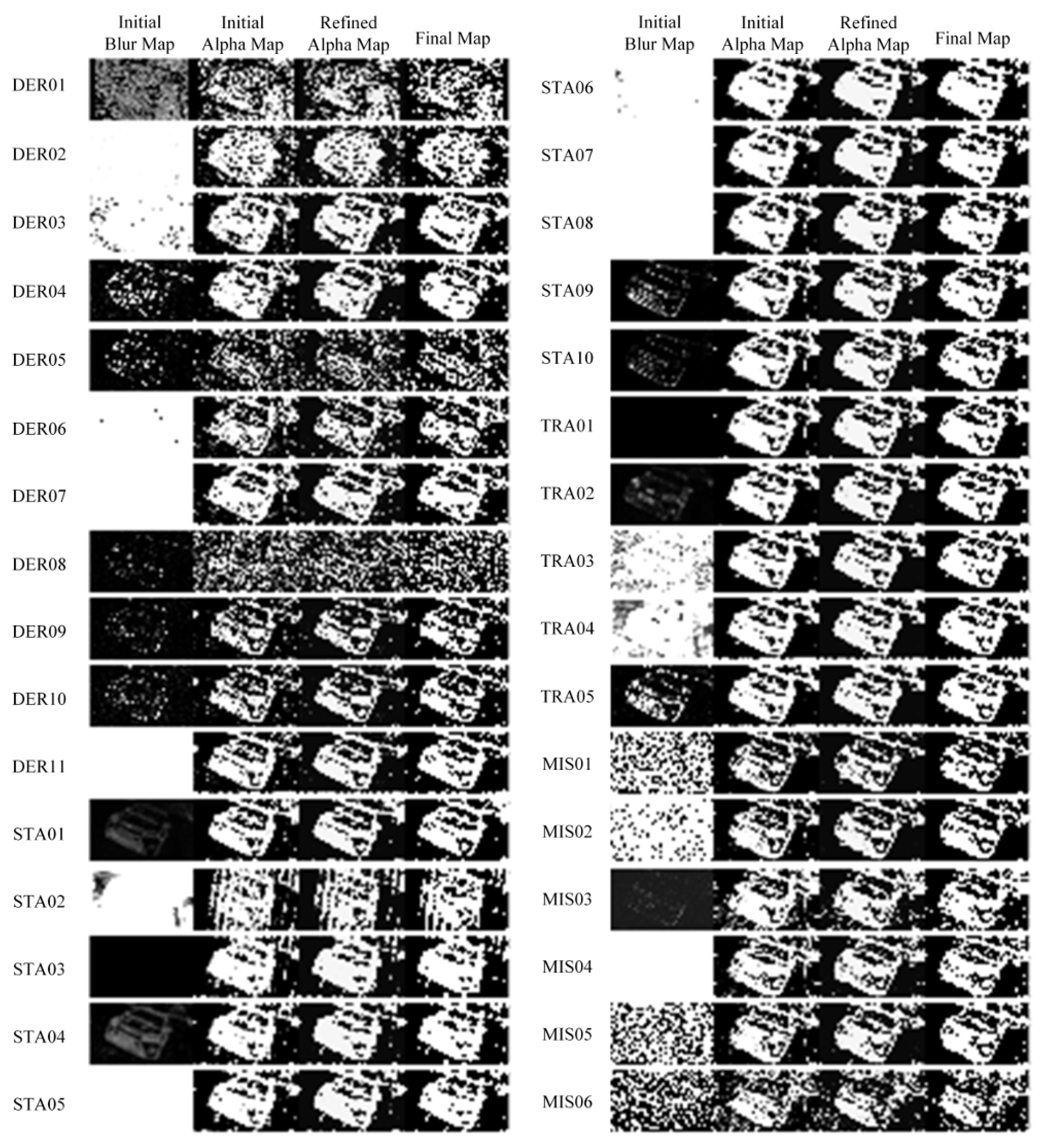
Figure 7.
Visual comparison of the performance of blur measure operators for defocus blurred image with and without salt and pepper noise. (a) From left to right: first, randomly selected image; second, its ground truth blur map; third to fifth, noisy variants of the original image corrupted with salt and pepper noise of density , and respectively. (b) Blur maps for the clean and noisy images.
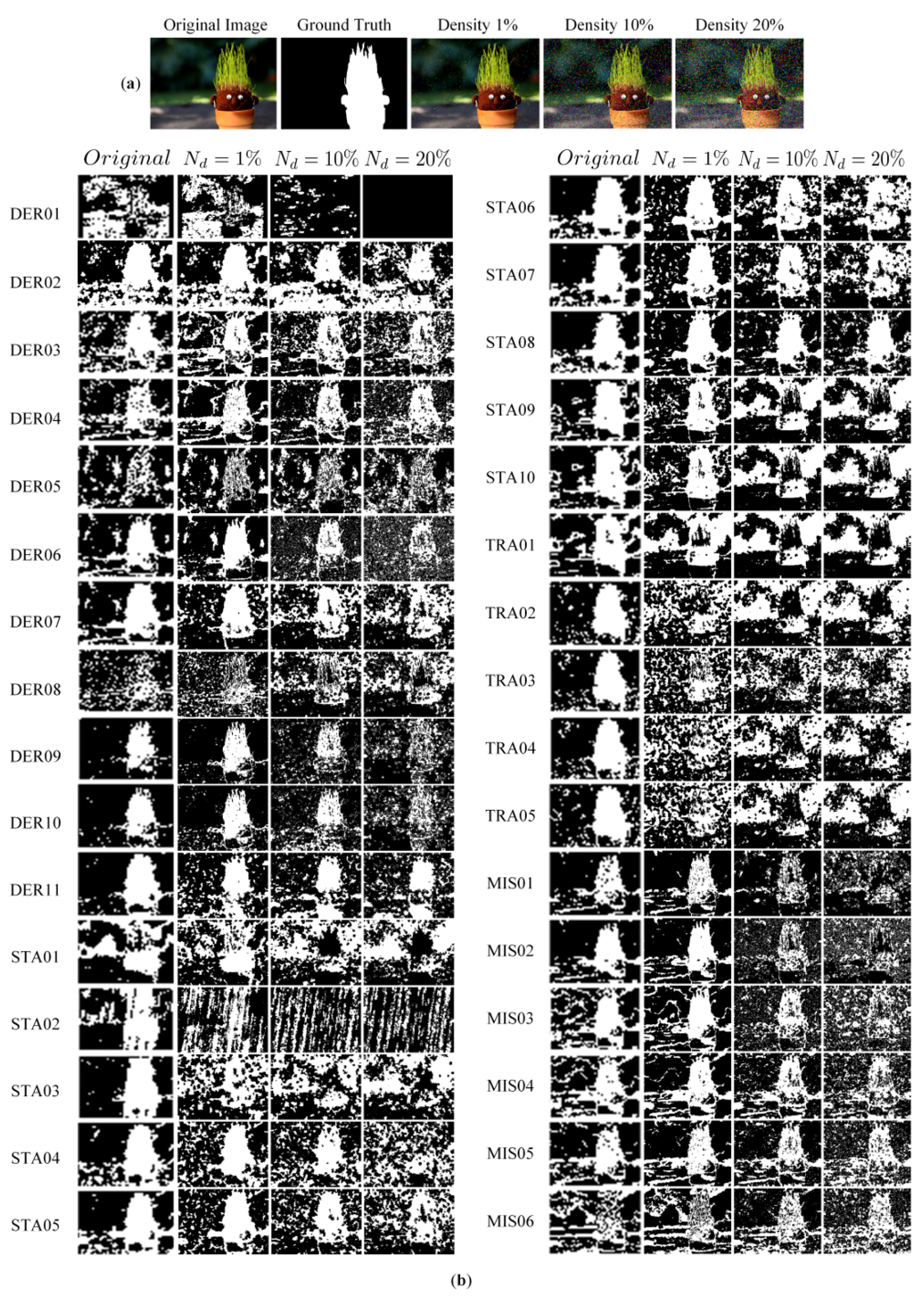
Figure 8.
Visual comparison of the performance of blur measure operators for defocus blurred image with and without random impulse noise. (a) From left to right: first, randomly selected image; second, its ground truth blur map; third to fifth, noisy variants of the original image corrupted with random impulse noise of density , and respectively. (b) Blur maps for the clean and noisy images.
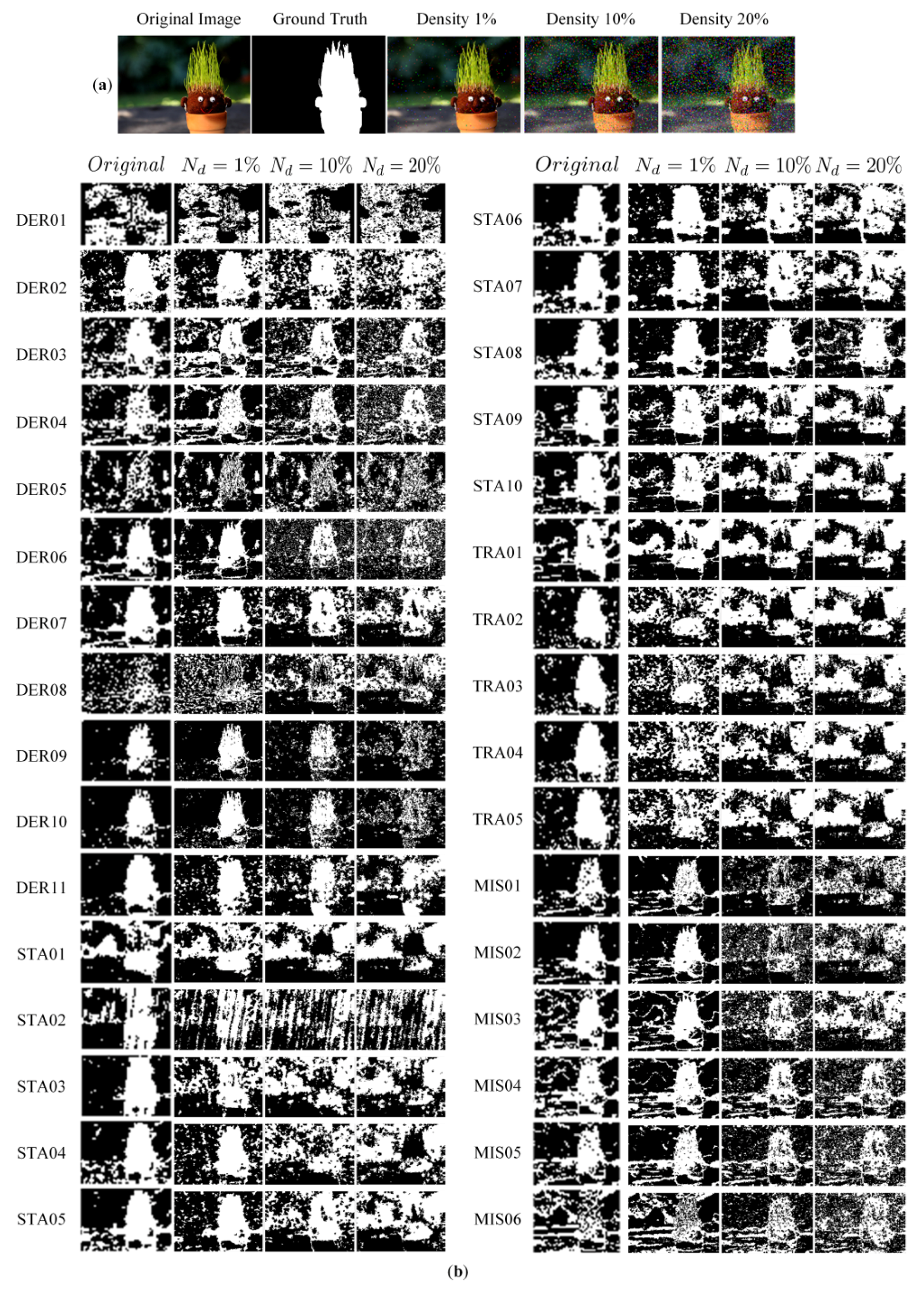
Figure 9.
Visual comparison of the performance of blur measure operators for motion blurred image with and without salt and pepper noise. (a) From left to right: first, randomly selected image; second, its ground truth blur map; third to fifth, noisy variants of the original image corrupted with salt and pepper noise of density , and respectively. (b) Blur maps for the clean and noisy images.
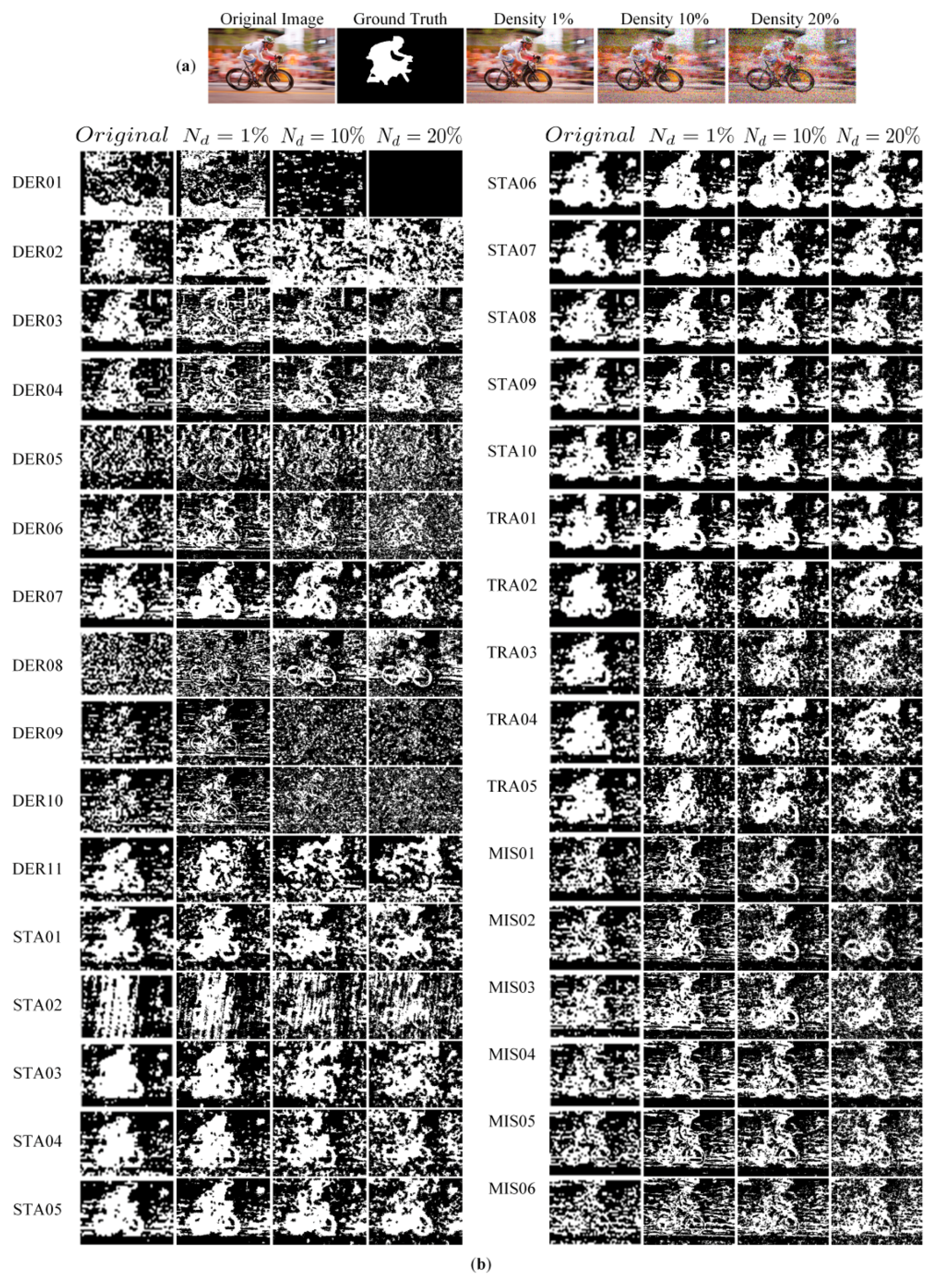
Figure 10.
Visual comparison of the performance of blur measure operators for motion blurred image with and without random impulse noise. (a) From left to right: first, randomly selected image; second, its ground truth blur map; third to fifth, noisy variants of the original image corrupted with random impulse noise of density , and respectively. (b) Blur maps for the clean and noisy images.

Figure 11.
Mean performance of the blur measure operators over 303 randomly selected images troubled by defocus blur.
Figure 11.
Mean performance of the blur measure operators over 303 randomly selected images troubled by defocus blur.

Figure 12.
Mean performance of the blur measure operators over 204 randomly selected images troubled by defocus blur and salt and pepper noise.
Figure 12.
Mean performance of the blur measure operators over 204 randomly selected images troubled by defocus blur and salt and pepper noise.
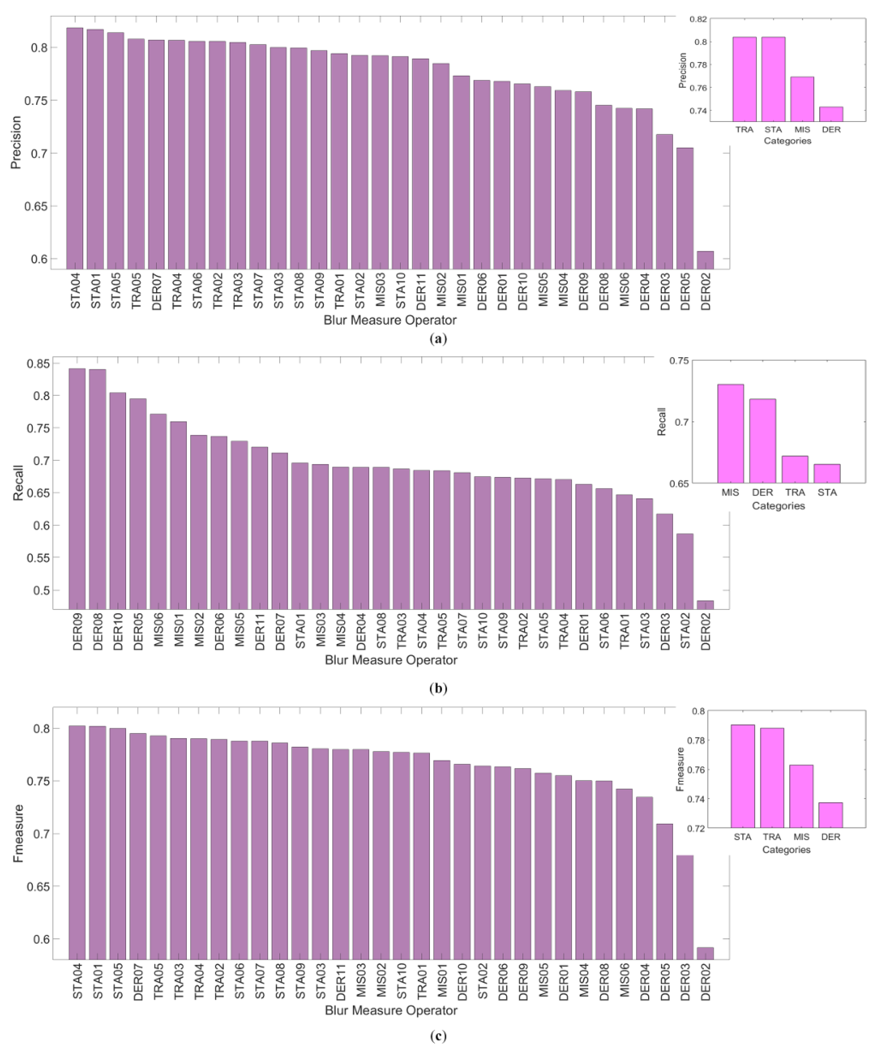
Figure 13.
Mean performance of the blur measure operators over 235 randomly selected images troubled by motion blur.
Figure 13.
Mean performance of the blur measure operators over 235 randomly selected images troubled by motion blur.

Figure 14.
Mean performance of the blur measure operators over 296 randomly selected images troubled by motion blur and salt and pepper noise.
Figure 14.
Mean performance of the blur measure operators over 296 randomly selected images troubled by motion blur and salt and pepper noise.

Figure 15.
Mean evaluation measures for blur measure operators in case of defocus blur.

Figure 16.
Mean evaluation measures for blur measure operators in case of motion blur.


Table 1.
Serial numbers and abbreviations to refer the blur measure operators.
| Sr. No. | Blur Operator | Abbr. | Sr. No. | Blur Operator | Abbr. |
|---|---|---|---|---|---|
| 1 | Gradient Histogram Span | DER01 | 17 | Gray-level local variance | STA06 |
| 2 | Kurtosis | DER02 | 18 | Normalized Gray-level variance | STA07 |
| 3 | Gaussian derivative | DER03 | 19 | Histogram entropy | STA08 |
| 4 | Gradient energy | DER04 | 20 | DCT energy ratio | STA09 |
| 5 | Squared gradient | DER05 | 21 | DCT reduced energy ratio | STA10 |
| 7 | Tenengrad variance | DER07 | 23 | Power spectrum | TRA02 |
| 7 | Tenengrad variance | DER07 | 23 | High-frequency multiscale Fusion and Sort Transform (HiFST) | TRA02 |
| 8 | Energy of Laplacian | DER08 | 24 | Sum of wavelet coefficients | TRA03 |
| 9 | Modified Laplacian | DER09 | 25 | Variance of wavelet coefficients | TRA04 |
| 10 | Diagonal modified Laplacian | DER10 | 26 | Ratio of wavelet coefficients | TRA05 |
| 11 | Variance of Laplacian | DER11 | 27 | Brenner’s measure | MIS01 |
| 12 | Singular value decomposition | STA01 | 28 | Image contrast | MIS02 |
| 13 | Sparsity of dark channel | STA02 | 29 | Image curvature measure | MIS03 |
| 14 | Total variation | STA03 | 30 | Steerable filters-based | MIS04 |
| 15 | Local binary pattern | STA04 | 31 | Spatial frequency | MIS05 |
| 16 | Gray-level variance | STA05 | 32 | Vollath’s autocorrelation | MIS06 |
© 2018 by the authors. Licensee MDPI, Basel, Switzerland. This article is an open access article distributed under the terms and conditions of the Creative Commons Attribution (CC BY) license (http://creativecommons.org/licenses/by/4.0/).
Share and Cite
MDPI and ACS Style
Ali, U.; Mahmood, M.T. Analysis of Blur Measure Operators for Single Image Blur Segmentation. Appl. Sci. 2018, 8, 807. https://doi.org/10.3390/app8050807
AMA Style
Ali U, Mahmood MT. Analysis of Blur Measure Operators for Single Image Blur Segmentation. Applied Sciences. 2018; 8(5):807. https://doi.org/10.3390/app8050807
Chicago/Turabian StyleAli, Usman, and Muhammad Tariq Mahmood. 2018. "Analysis of Blur Measure Operators for Single Image Blur Segmentation" Applied Sciences 8, no. 5: 807. https://doi.org/10.3390/app8050807
Note that from the first issue of 2016, this journal uses article numbers instead of page numbers. See further details here.