Fisher Discriminative Sparse Representation Based on DBN for Fault Diagnosis of Complex System

School of Automation, Chongqing University, Chongqing City 400030, China
*
Author to whom correspondence should be addressed.
Appl. Sci. 2018, 8(5), 795; https://doi.org/10.3390/app8050795
Submission received: 23 January 2018
/
Revised: 16 April 2018
/
Accepted: 17 April 2018
/
Published: 16 May 2018
Abstract
:Fault detection and diagnosis in the chemical industry is a challenging task due to the large number of measured variables and complex interactions among them. To solve this problem, a new fault diagnosis method named Fisher discriminative sparse representation (FDSR), based on deep belief network (DBN), is proposed in this paper. We used DBN to extract the features of all faulty and normal modes. Features extracted by the DBN were used to learn subdictionaries, then the overcomplete dictionary was constructed by cascading all subdictionaries in order, and each dictionary atom corresponded to class labels. The Fisher discrimination criterion (FDC) was applied to the dictionary learning to ensure smaller within-class scatter but greater between-class scatter. The quadratic programming method was applied to estimate the sparse coefficients simultaneously class by class. Therefore, both the reconstruction error and sparse coefficients were discriminative, so that the reconstruction error after sparse coding can be used for pattern classification. An experiment performed on the Tennessee Eastman (TE) process indicated that compared with the traditional monitoring methods, the FDSR based on DBN produced more interpretable results and achieved superior performance for feature extraction and classification in the field of complex system fault diagnosis. T-distributed stochastic neighbor embedding (t-SNE) appropriately visualized the performance of the proposed method and produced reliable fault diagnosis results.
1. Introduction
With the increase in the complexity of operation and multiloop control processes, a robust fault detection and diagnosis (FDD) method has become increasingly necessary for industrial processes. Fault detection and diagnosis involves developing a method that detects faults quickly, diagnosing the fault type, and determining the root causes of the fault with the least number of false alarms [1,2]. A good fault detection and diagnosis system not only guarantees the quality of the product but also improves the safety of the system.
Fault diagnosis methods are categorized into data-based, model-based, knowledge-based, and hybrid methods [3]. Knowledge-based methods are mature and we do not discuss them here. Model-based methods have been proposed by Beard (1971) to replace hardware redundancy with analytical redundancy, and Willsky (1976) proposed the key concepts of analytical redundancy for model-based fault detection and diagnosis. Next, parameter estimation, observer-based algorithms, and parity space methods were introduced and later improved. They were used to solve the control problem in heating, ventilating, air conditioning, motor, and engine systems [3,4]. Based on the model constructed using the physical principles and system identification techniques, fault diagnosis methods were developed to monitor the error between the outputs of practical systems and model-predicted outputs [5,6,7,8,9].
Generally, obtaining an explicit model to accurately describe the dynamic behavior of a complex system is difficult, and model-based algorithms [3,5,6,7] have considerable limitations. Due to the extensive applications of modern measurements and the quick development of data analysis methods, data-driven process monitoring techniques have attracted the attention of experts [9,10,11,12,13]. Many fault detection and diagnosis methods have been proposed based on some widely used dimensionality reduction techniques, such as partial least squares (PLS) [14], independent component analysis (ICA) [15], principle component analysis (PCA) [16], and locally preserving projections (LPP) [17]. These multivariate statistical process monitoring (MSPM) methods are commonly used to extract features based on the established distribution, determine the latent variables, and then construct a monitoring model using the extracted features for fault detection and diagnosis.
One common drawback of the above dimensionality reduction methods is that the extracted features are the linear combination of all input variables. Furthermore, the lack of sparsity in the features hides the physical connection of complex systems. To reveal the deeper connection between the variables and create a proper representation of physical meaning, this paper proposes a novel feature extraction scheme for complex system fault diagnosis using deep learning and sparse representation. Deep learning allows computational models composed of multiple processing layers to learn the representation of data [18,19,20,21]. The backpropagation algorithm (BP algorithm) is applied after the weights training step in deep learning to discover intricate structures in large data sets, and the BP algorithm makes up the disadvantage of gradient diffusion in pretraining weights of the network.
The convolutional neural network proposed by Lecun was the first deep learning algorithm that trained multilayer networks successfully, but it was not sufficiently effective during application. A breakthrough in deep learning occurred in 2006 when Hinton introduced the deep belief network (DBN), a novel deep learning architecture [18]. Since then, ever-increasing research has been performed in the fields of pattern recognition, computer vision, and data mining. Zhao et al. applied DBN to fault feature extraction and diagnosis of bearings and introduced PCA to extract two principle components for visualization [22]. The authors determined the DBN can both extract the features of fault types in single work conditions and the features of blended conditions. Wang combined a particle swarm optimization algorithm with DBNs to particle DBNs (PDBNs), and determined the PDBN model with optimized network parameters performed better and had higher identification precision [23]. To take advantage of DBNs and quantum inspired neural networks (QINN), Gao et al. proposed the linear superposition of multiple DBNs with quantum intervals in the last hidden layer to construct a deep quantum inspired neural network and applied it to the fault diagnosis of aircraft fuel systems [24]. To decrease the DBN pretraining time, Lopes proposed two complementary approaches. An adaptive step size technique was first introduced to enhance the convergence of contrastive divergence algorithms, and then a highly scalable graphics process unit parallel implementation of the CD-k algorithm was presented, which notably increased the training speed [25]. Mostafa et al. proposed a novel supervised local multilayer perceptron classifier architecture integrated with ICA models for fault diagnosis and detection of industrial systems. The Expectation-Maximizing clustering technique was applied to improve single neural network (SNN) classifiers. The effectiveness of the proposed method was illustrated with the Tennessee Eastman (TE) process [26].
Since the deep belief network extracts features layer by layer, it has unique advantages in the feature extraction of high-dimension and nonlinear data processing. Additionally, the TE process is a complex industrial process with many variables and a large amount of data. To reduce the dimension of variables and determine the relationship with interpretability, we introduced deep belief networks to extract features of raw data from industrial processes.
The other drawback of the above dimensionality reduction methods is that they are based on a statistical model, which assumes the probability distribution of the process variables first, and then sets the corresponding threshold to complete fault diagnosis, whereas the accuracy of the methods mostly depends on the threshold and statistical model. To create more interpretable results and promote better generalization, we introduce Fisher discrimination sparse representation (FDSR) to diagnose faults that can be seen as a supervised classification task, the target of which is to assign new observations to one of the existing classes. Various supervised learning models have been introduced, such as error propagation, deep neural networks [27], support vector machine (SVM), and logistic regression. Deep neural networks perform well when sufficient normal and fault data are available, whereas the features extracted by DBNs are dimension reduced, meaning there is insufficient input data for deep neural networks. SVM, another efficient classifier, performs well with limited training data, whereas the lack of a rejection mechanism limits the application in fault diagnosis, especially for some industries such as nuclear areas and chemical processes with high danger probability [28].
Sparse representation is widely used in pattern recognition, image processing, and fault diagnosis [29,30,31,32,33,34,35], since it can include danger rejection as a restriction in the representation model and iterate training data to learn the discriminative dictionaries. Then, the corresponding sparse coefficients can be used to perform fault diagnosis in a complex system. Yu et al. proposed a sparse PCA algorithm for nonlinear fault diagnosis and robust feature discovery in industrial processes, with the robustness of this method being proved with the TE process [29]. To study the relationship between monitoring parameters and faults, Bao et al. proposed a new sparse dimensionality reduction method called sparse global-local preserving projections, which greatly improved the interpretability of fault diagnosis [30]. Wu et al. proposed a novel fault diagnosis and detection method based on sparse representation classification (SRC), with the main contribution being the model training and multiclassification strategy [31].
To determine meaningful correlations among variables, the DBN was introduced to solve the redundant coupling problem and eliminate interference between process variables. This paper proposes a novel FDSR framework as the classification model to solve the classification of dimension-reduced features. To solve the classification problem with strong coupling and danger rejection limitation in modern industrial processes, the discriminative subdictionaries were learned corresponding to class labels, and the overcomplete dictionary was constructed by cascading subdictionaries orderly. Then, fault diagnosis was completed by determining the smallest reconstruction error, since the dictionary and coefficient are both sparse. The results are then compared to the backpropagation (BP) network, conventional sparse representation, and support vector machine. The advantages and efficacy of the proposed methods are illustrated by a case study on the TE process.
The rest of the paper is organized as follows. Section 2 reviews the DBN techniques for feature extraction, which includes both the theory and their application in feature extraction. Section 3 provides a detailed illustration of the FDSR and the idea behind fault diagnosis. Section 4 introduces an overview of the proposed fault diagnosis methodology, then describes the experiment procedure and the datasets. The performance of the proposed method is also evaluated in this section. Finally, Section 5 summarizes the present research and potential future work.
2. Deep Belief Networks (DBNs)
DBNs are typical deep neural networks, which are stacked by a number of restricted Boltzmann machines (RBMs). The RBM structure is shown in Figure 1. RBM intelligently transform the features in raw space, layer by layer, into abstract representations in a new space, which reflects the distribution of the samples with certain desirable properties and avoids human interference in feature extraction. Compared with stacked auto-encoder, DBNs can simultaneously have lower reconstruction error with more information. The DBN first adjusts the parameters with larger partial derivatives of time complexity, which reduces the calculation cost of the network. Convolution neural network (CNN) is another important deep network that includes a convolutional layer and a pooling layer. CNN is applied to features that are spatially related, like in image processing, whereas the samples from industrial processes are time series, which are not suitable for fault diagnosis in industrial processes.
The DBN process first pretrains the weights of every layer with unsupervised learning, then fine tunes the weights from top to bottom to obtain the optimal model, in which the weights between the output layer and the layer before it can be recognized as the feature of the input data. The DBN process is suitable for big data analysis with successful applications to pattern recognition, computer vision, music audio classification, and recommendation systems [36,37,38,39]. DBN learns the features of the original signal, layer by layer, using an unsupervised greedy algorithm. Then, the features from the original space are represented in a new space. This network automatically learns to obtain a hierarchical feature representation with more classification guidance and feature visualization. Deep learning not only has stronger representation ability and faster calculation speeds compared with a classifier with a superficial structure, but also can solve problems of overfitting and local optimization effectively [40]. These advantages make deep learning perform well in solving the redundant coupling and connection problems among the variables of the complex system.
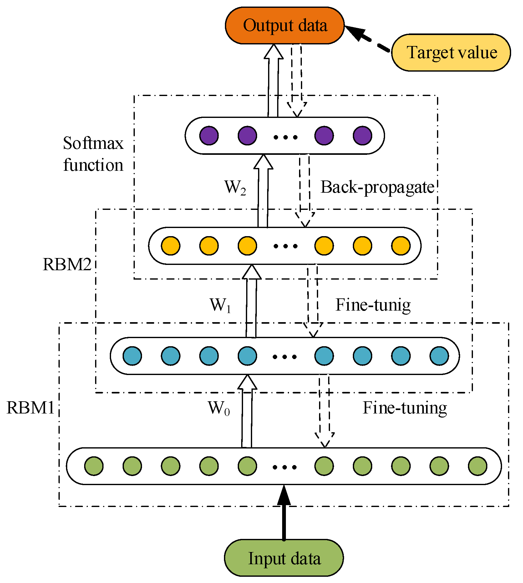
The RBM was first proposed by Smolensky, and has been prominent since Hinton stacked a bank of RBMs to construct DBNs in 2006 [40]. RBMs are based on energy, in which the inputs are considered as a probability distribution. An RBM is a special type of Markov random field with stochastic visible units in the visible layer and stochastic observable units in the hidden layer. As shown in Figure 2 the visible layers are fully connected with hidden layers, but there are no connections among the visible layer or the hidden layer. The equations in the left part of Figure 2 show the forward pass in a DBN with six input nodes in the visible layer and two hidden layers with two output nodes in output layer. The first hidden layer has four nodes and the other has three. Each constitutes a module through which the gradients can be backpropagated. We first computed the total input z of each node, which is the weighted sum of the outputs from the last layer. Then, a nonlinear function was applied to z to obtain the output of this node. By computing layer by layer, the output of DBN can be obtained. The right part of Figure 2 shows the gradient calculation of the backward pass, in which is the target value. Notably, the computation of the error derivative starts from the outputs to the inputs, which is contrary to the forward pass. With the solution of maximum gradient, we can obtain the optimal weights of this network.
For any given set of state in an RBM model, the energy function is defined as
where and represent the number of neuros in the visible and hidden layer, respectively; and are the state vector of neurons in the visible and hidden layer of the model, respectively; and are the bias of neurons; and is the weight matrix of the units between the visible and hidden layers. Then is the parameters set of the RBM model, which is the goal matrix of our training. Then the joint probability distribution function of state is calculated according to
where is a partition function. The probability distribution of the observed data is the practical concerns, which is also the edge distribution of , recognized as the likelihood function as follows:
Similarly:
According to the Bayes and sigmoid function, the neuron in the visible (hidden) layer is activated, with a value of 1, given a full state of neuros in the hidden (visible) layer by the probability ().
The training goal was to determine parameter to ensure the output of RBM was as similar as possible to the maximum of the likelihood . Since the log-likelihood gradient was initially equal to the components, the target can be translated to maximize the function . Notably, the training process is more efficient when using a gradient descent based on the contrastive divergence (CD) algorithm to optimize this question. Then, the weighting matrix can be updated according to Equation (7). The detailed proof can be seen in a previous study [40]. To enhance the learning rate and accuracy, Mnih et al. proposed a more practical algorithm named persistent contrastive divergence [41], which traced the states of persistent chains instead of searching the initial value of the Gibbs Markov chain at the training data vector.
DBNs are a cascade connection of stacked RBMs and are composed of multiple layers of stochastic and latent variables, which can be considered a special form of the Bayesian probabilistic generative model. The schematic diagram of the DBN model is shown in Figure 3. The hidden and visible layers are connected in order. Hinton proposed a greedy layer-wise learning algorithm to train the model from bottom to top and train only one layer at a time, with the parameters of the other layers being fixed. The outputs of layer are the input of layer used to train until the top level is reached. This is called the pretraining or feature-learning process, which determines the independent parameters in every RBM of the DBN. After the learning of the optimized weights is finished, the parameter optimal algorithm is usually backpropagated to determine the global optimal. This is called the fine-tuning process, which is supervised learning from top to bottom [42]. Figure 3 shows the learning flowchart of the DBN model.
3. Fisher Discriminative Sparse Representation (FDSR) of the Features Extracted from DBN
3.1. Sparse Dictionary Constructed Based on Fisher Discriminative Dictionary Learning
In the quest for the proper dictionary to use in fault classification, preconstructed dictionaries, adapted dictionaries, and redundant dictionaries are recognized as three options of dictionary learning. Preconstructed dictionaries, such as steerable contourlets, wavelets, and curvelets, are tailored specifically to imaging, and in particular, to stylized cartoonlike image content. Alternatively, adapted dictionaries such as wavelet packets and bandelets provide a tunable selection of a dictionary, in which the basis or frame is generated under the control of a particular parameter. The wavelet packets introduced by Coifman et al. assumed control over the time-frequency subdivision, tuned to optimize performance over a specified instance of a signal. The bandelets introduced by Mallat et al. were spatially adapted to better treat images by orienting the regular wavelet atoms along the principal direction of the local area processed [43]. The Method of Optimal Directions (MOD) and K-singular value decomposition (K-SVD) [44,45] are popular dictionary learning algorithms. Fisher discriminative dictionary, using three dictionary training mechanisms, has attracted considerable attention.
To improve the performance of previous deep learning methods, we propose a novel Fisher discrimination dictionary in this study. Instead of learning a sharing dictionary for all classes, we learned a structured dictionary , where c is the total number of classes, and is the subdictionary that is class-specific and associated with class . Apart from requiring powerful reconstruction capability of , also should have powerful discriminative capability of .
To obtain the sparse representation of the signal, an overcomplete dictionary is often learned from training samples based on the sparse model. The dictionary and sparse coefficients are key for the sparse representation of the signal. K-SVD is not suitable for classification tasks because it only requires that the learned dictionary to accurately represent the training data, but not necessarily have classification characteristics. To improve the performance of the classification ability, we propose a novel Fisher discriminate dictionary . We get the features from DBNs, in which is the subset of features from class , which is then used as the training samples to construct 22 subdictionaries. These subdictionaries are the representation of 21 fault types and one normal condition, and they are sequentially concatenated columnwise to form an overcomplete dictionary to fully represent all states of TE process. Denoted by , where the coding coefficients are over and is the submatrix containing the coding coefficients of . should be able to reconstruct effectively. Additionally, can represent samples of class sparsely with minimal error, whereas cannot. That is, has powerful discriminative ability for signals in . As such, we propose the discriminative dictionary learning model:
where and are scalar parameters, is the Fisher discriminative fidelity term, which limits the learned dictionary , which optimally represents , and and are the sparse constraint and discrimination constraint applied to coefficient matrix , respectively.
As the optimal dictionary to represent :
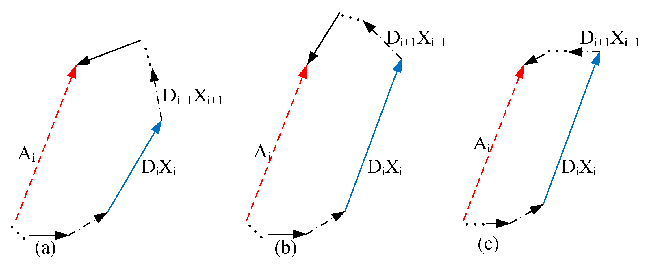
where is the representation of in the dictionary , and is the representation of in the dictionary . The Fisher discriminative fidelity term includes three parts: (1) The structured dictionary should be able to well represent , meaning is small; (2) Dictionary in Figure 4a satisfies this claim. Then, the subdictionary that corresponds to is optimal in . This limitation can be represented as a mathematic function: , which is small enough. Figure 4b shows this constraint; (3) should have nearly zero coefficients so that representation are small enough, as shown in Figure 4c. Above all, the Fisher discriminative fidelity term [46] is as follows:
The idea above limits the discrimination of the dictionary. We defined to constrain the discriminative of the sparse coefficient . Learning from the criterion, such as the Fisher discriminative criterion, we introduced between-class scatter and within-class scatter to illustrate the discrimination of . Within-class scatter is recognized as the sum of distance between column vectors in the coefficient matrix that correspond to class i and the mean vector of . Between-class scatter is defined as the sum of the distance between the mean vector of and the mean vector of multiplied by the number of vectors in . and are defined as:
Denoted by and , to ensure the convex and stability of , we introduced an elastic term and a scalar parameter into . Then, is defined as:
The definition of the discriminative of dictionary D and sparse coefficient ensure both dictionary and coefficient can be applied to fault diagnosis. Then, we have the FDSR model:
3.2. Optimization of the Fisher Discriminative Sparse Representation
The FDSR target function is not jointly convex to ; it is convex to each and , whereas the other is fixed. This promotes the alternative optimization algorithm, a sparse coding problem that optimizes while D is fixed. Optimizing while is fixed is a quadratic programming problem.
First, we initialized , applying principle component analysis (PCA) to the feature extracting results of DBN. PCA maps data into a new dimensional subspace that contains that most varied data to ensure the least information loss. An m-dimensional data set includes samples, which is given as , where are the score vectors or principal components (PCs), are loading vectors, is the score matrix, and is the loading matrix. Here, we used PCA only to initiate the dictionary but not to reduce the dimensions, so we chose training data from class to obtain PCs , and the matrix included in the corresponding subdictionary , in which the initialized dictionary included 100% of the principal components.
Then, we assumed was fixed. The objective function in Equation (14) was reduced as a sparse coding problem to calculate , as shown in Equation (15), which can be solved using a match pursuit algorithm. In this paper, we solved coefficient class by class. After updating coefficient , we fixed by reducing Equations (13) to (16) to update subdictionary class by class:
where is the coding coefficient of over .
To ensure the convexity and discrimination of , we set . Then, all terms except are differentiable. Equation (15) can be solved using the iterative projection method proposed by Rosasco et al. [46] (Appendix A). Notably, each column of dictionary should be a unit vector. Equation (16) is a convex optimization problem that can be solved using the algorithm proposed in Yang et al. [47], (Appendix B). The FDSR algorithm is shown in Table 1.
3.3. Fault Diagnosis Solution
Since the dictionary and sparse coefficient are solved above, the diagnosis of the fault type is based on minimizing the reconstruction error. We performed classification using , where , and is the coefficient corresponding to subdictionary . Here, we introduced the norm of X to ensure the sparsity of the coefficient, if the number of non-zero atoms not small enough, the dictionary cannot be the optimal candidate.
3.4. Computation of Fisher Discriminative Sparse Representation
The computation of FDSR is mainly divided into three steps: DBN training, eigenvector solving, and dictionary learning. In this paper, the DBN consists of three RBMs, set neuros in each RBM as , and , the inputs are samples with parameters, is the number of iterations. The computational complexity of the first, second, and third RBM can be represented as , and respectively, and the computational complexity of fine tuning is defined as .
Then, the computational complexity of DBN is:
is the iterations of FDSR method with sparsity , then the computational complexity of dictionary learning and eigenvector solving is , , respectively. As a result, the complexity of FDSR is .
4. Case Study
The FDSR method based on a deep neural network was applied to the TE process. The flowchart of the TE process is shown in Figure 5, with a plantwide control structure proposed by Lyman and Georgakis. The structure describes the nonlinear relationship among devices, materials, and energy. The system includes five major unit operations: an exothermic two-phase reactor, a vapor-liquid flash separator, a product condenser, a recycling compressor, and a reboiled product stripper. Four gaseous materials are involved, A, C, D, and E, with products G and H having a byproduct of F. In addition, inert gas B is added to the reactants. First, A, D, and E are fed into the reactor, then the products are sent into the condenser. The condensed product flows to a vapor-liquid flash separator, in which the products that have not yet been compressed are recycled by the compressor and sent to reactor, whereas the gases that has been compressed are sent to the stripper to remove the remaining reactants. Then, the byproduct F and inert gas B are removed by the purge valve to obtain products G and H.
Downs and Vogel [48] developed a simulator for the TE process, allowing 21 disturbances (faults), 12 manipulated variables (XMV1 to XMV12), and 41 measured process variables, of which 22 are continuously monitored process variables (XMEAS1 to XMEAS22) and 19 are composition measurements (Table 2). Detailed descriptions of this process can be found in Wu et al. [44]. In this case study, the 22 continuously monitored variables (Table 2) and 11 manipulated variables were monitored for online fault diagnosis with the agitation speed set to 50%. Six kinds of operating modes were possible. We completed the simulation under the first mode, which is the basic mode. The normal datasets were sampled under normal operating conditions, and 21 fault datasets were generated under 21 types of faulty operating conditions, as shown in Table 3. The faults in bold were chosen to test the effectiveness of the proposed algorithm. Faults 16 to 20 were unknown types. Faults 1 to 7 were associated with step variation, faults 8 to 12 were the random causes of variations in the process variables, whereas slow drift caused fault 13, and the sticking leads were faults 14, 15, and 21. In this case study, we used the PI cascade control structure proposed by Downs [48], and the data were sampled every 3 min. Each dataset contained 960 samples. The fault was introduced into the process after the 161st sample. The task defined here was to diagnose different working conditions based on the process data.
4.1. Overview of the Proposed Fault Diagnosis Algorithm
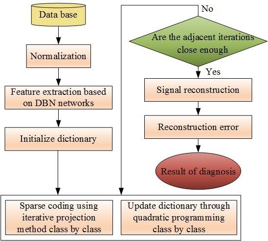
To improve the calculation speed of the sparse coefficient solution and make the sparse representation more suitable for high-dimension industrial process data, the proposed fault classification algorithm was developed based on DBNs and sparse representation. As shown in the flowchart in Figure 6, the training data was first preprocessed by normalization, then the features were extracted from various classes with the DBNs drawing on the idea of dimension-reduction.
Then, various features were trained with FDSR limitation to obtain the redundant subdictionaries, which were cascaded to construct the discriminative dictionary. The parameters of FDSR chosen by cross-validation are , , with 1000 iterations, 125 iterations for each case. We also did experiments on eight cases which are the faults in bold in Table 3 (including the normal case, fault 1, fault 6, fault 8, fault 12, fault 13, fault 14, and fault 18). The subdictionary is initialized by PCA and acquired 22 × 960 matrix, and the sparse level is set to 21. In addition, the Fisher discrimination criterion was applied to dictionary learning to ensure the discrimination of both sparse coefficients and subdictionaries. First, the FDSR restricted the larger among-class scatter and smaller within-class scatter. Then, we created each class-specific subdictionary to best represent the training samples from the associated class, but this subdictionary poorly represented the samples from the other classes. Both ensure the discrimination of the sparse coefficients and the reconstruction error. Additionally, the sparse representation coefficients of the extracted features were resolved using the iterative projection algorithm. Once the coefficients and dictionaries were acquired, the reconstruction error between samples of class-specific and other classes could be calculated. Furthermore, the fault type corresponded to the dictionary with the smallest error. The DBN-FDSR method was applied to the TE process to validate its performance.
4.2. Feature Extraction Results
Since the TE process has 53 parameters, the deep neural network extracts features as a filter with 53 input perceptrons and two hidden perceptrons. The input-to-hidden layer is fully connected and there are no connections among the layer itself. The connections can be recognized as a filter since they eliminate useless information from inputs while maintaining information that reflects certain fault information. Through this method, the DBN trained with two hidden layers can be considered as a feature extractor to determine the optimal features of the classes. The DBN parameters were set to 52 × 20 × 16 × 22, in which 52 was the input dimensions of the TE parameter, 20 and 16 are the output dimensions of the first hidden layer and second layer, respectively, and 22 is the total number of classes in the process with 21 fault types and the normal condition.
The DBN was trained with 10,560 samples from the normal condition and 21 fault cases, in which every case had 480 samples. So that the weight matrix visualization would be more direct and comparable, these connections were horizontally folded into 10,560 × 50, 10,560 × 20, and 10,560 × 16 pixels. Figure 7 shows the weight matrix acquired from training the DBN. Given space restrictions, we chose 40 sample data points from eight cases, which included the normal case, fault 1, fault 6, fault 8, fault 12, fault 13, fault 14, and fault 18. The eight cases included all fault types (step, random, slow drift, sticking, and unknown faults). Since the fault was introduced in the 161st sample point, we chose from 161 to 200 as the 40 samples points (Figure 7). The first column in Figure 7 is the raw data of the above eight cases, and the second column is the output of the first hidden layer. Since the parameters were set as 52 × 20 × 16 × 22, the output of the first hidden layer was 10,560 × 20. The third column is the output matrix of the second hidden layer with a dimension of 10,560 × 16. The difference between the weight matrix is the magnitude of its value, i.e., color depth. This demonstrates that the different running statuses contain various characteristics that can be considered fault features, such as the vectors addressed in the red box in Figure 7. Hidden 1 of fault 1 is the same as fault 14 in the green box in the second column of Figure 7. After the transformation of the second layer, the weight changed as shown in the green box of the third column, which can be used to complete feature extraction in complex systems. It also provides a fault diagnosis method with sparse representation.
All of these techniques were implemented on the MATLAB 2016a platform on a personal computer with an i5-6500 core CPU at 3.20 Ghz, and 8 GB of RAM. Feature extraction from the training data required 8 min and 5 min to extract the features of the testing data. The subdictionary learning was time consuming, requiring about 27 h to learn the 22 subdictionaries and sparse coefficients.
4.3. Comprehensive Comparison of Classifier Performance
To illustrate the discrimination ability of our algorithm, DBN [22], backpropagation (BP) [39], SVM with RBF kernel [28], and sparse representation (SR) classifiers [49] were compared with the FDSR proposed in this study. The neural numbers of DBN were set to 52 × 20 × 16 × 22 and kept the same in all tests. The parameters of SVM were optimized and the optimal and were acquired. The parameters of backpropagation were set to 52 × 30 × 22. More detail about these methods can been seen in the corresponding references. The classification test was repeated 30 times, and the average classification accuracy is summarized in Table 4. Fault 14 and fault 18 had the lowest accuracy in every classifier, proving the challenge posed in diagnosing unknown faults and sticking faults. The FDSR results were considerably better compared with other methods, verifying the superior clustering and separating ability of this methodology.
Performance of these various classification methods were evaluated based on Accuracy (Acc), Sensitivity (Sen), and Specificity (Spe). TP is the number of healthy data correctly recognized, TN is the number of faulty data correctly recognized, FN is the number of faulty data detected as healthy, and FP is the number of healthy data detected as faulty. Acc is the proportion of true decisions in all tests, and Sen and Spe represent the proportion of positive and negative cases that were detected correctly, respectively. The formulation is shown in Equations (19)–(21). We used Sen to evaluate the classification accuracy of these methods.
The comparison of the various classifiers and their accuracies are illustrated in Table 4. The proposed FDSR was superior, having the highest accuracy in all scenarios. The FDSR performs quite better than the traditional sparse representation classifier (SRC) [49], which could be attributed to the added constraints that limit the scattering of the samples within a class and maximize the scatter of samples between classes. Meanwhile, FDSR had higher reconstruction accuracy than SRC, due to the introduction of minimizing the reconstruction error restriction via L2 norm. The results demonstrate that FDSR is the optimal method for diagnosing faults compared with the other available methodologies.
4.4. Visualization of Learned Representation
To demonstrate the efficacy of the proposed FDSR based on DBN for feature extraction and diagnosis in industrial systems, we introduced the visualization technique called t-distributed stochastic neighbor embedding (t-SNE) [50,51]. T-SNE is a tool for dimensionality reduction that is well-suited for the visualization of high-dimension datasets. We chose faults 1, 2, 6, 8, 12, 13, 14, and 18 (Bold fault types in Table 3) and the normal data to complete the experiment. Step, random, slow drift, sticking, and unknown fault types were included to fully reflect the efficacy of the FDSR algorithm.
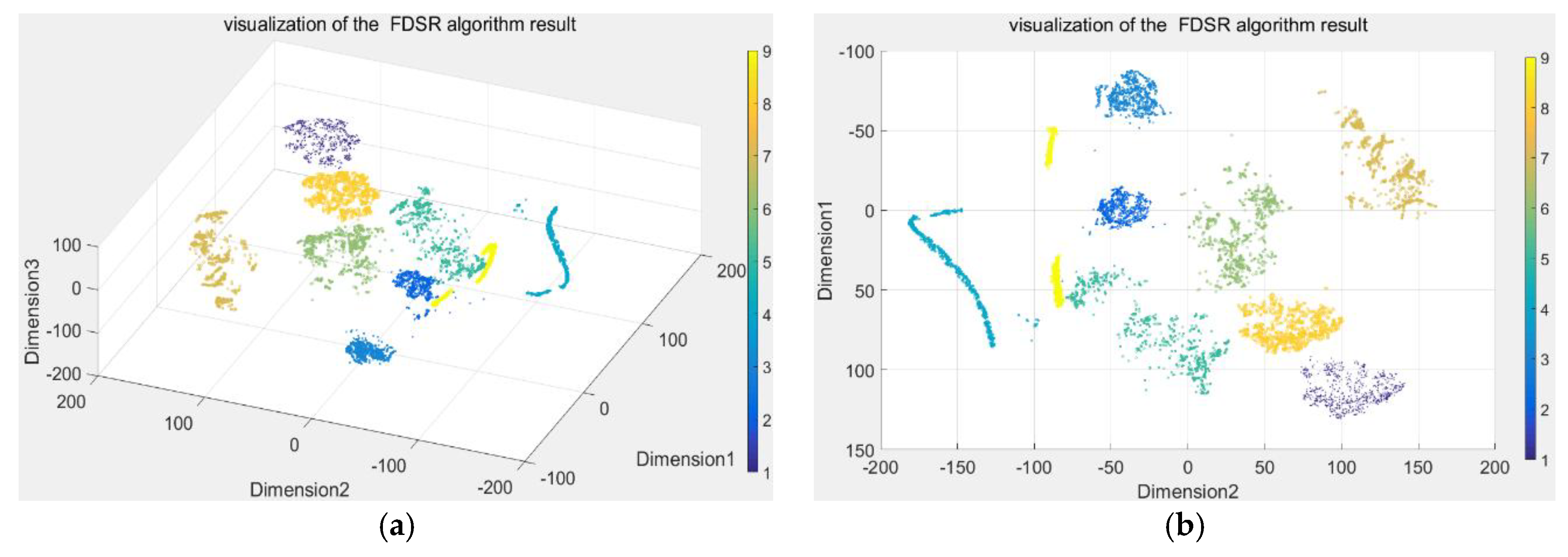
Here, the DBN was used to extract the features with 16 dimensions from raw process data, hasten the dictionary learning, and eliminate redundant information for diagnosis. Then, t-SNE, the dimension reduction technique, was used to convert the 16-demensional features to a three-dimensional (3D) map. The resulting scatterplot maps are shown in Figure 8. To better demonstrate the visualization of the clustering performance, Figure 8b is the 3D view at an azimuth of 90 degrees and a top view of 90 degrees, and Figure 8a is the view at an azimuth of −37.5 degrees and a top view of 30 degrees. Furthermore, the features were used to learn the dictionary with 176 dimensions using the iterative projection method. The discriminative sparse coefficients were updated using the quadratic programming algorithm. Then, we applied t-SNE to convert the discriminative coefficients to a 3D map and the resulting scatterplot maps are shown in Figure 8. We used the same technique to visualize the raw process data shown in Figure 9. Only three conditions were completely separated, and the remainder are indistinguishable in Figure 9. The features extracted by DBN were also poor, with four conditions separated completely, as shown in Figure 8. The coefficients acquired from FDSR clustered best where the data points of nine conditions were well-separated in Figure 10. This verifies the good classification ability of the FDSR algorithm investigated in this study. The result also indicates that faults 12, 13, 14, an 18 are hard to classify without an effective method, whereas the FDSR algorithm investigated here solved this problem well. This also verifies in the classification accuracy of the different conditions displayed in Table 3.
From the trends shown by the three maps (Figure 8, Figure 9 and Figure 10), the DBN itself is an effective feature-extraction method for industry process fault diagnosis. The FDSR based on the DBN approach, where the features are learned by DBN, appreciably improved the representation performance. The results also validate the superior classification performance of the FDSR algorithm based on DBN compared with other methods. Therefore, an FDSR-based deep neural network is an effective approach for industrial process fault diagnosis.
5. Conclusions
This paper proposed a novel FDSR algorithm based on the feature extraction of DBN for fault diagnosis. Deep learning was introduced to solve the multiparameters problem of complex systems, extracting features layer by layer with dimension reduction. FDSR is an improved sparse representation method that takes advantage of sparse representation and Fisher discriminant analysis. Then, the FDSR algorithm was proposed to learn a discriminative structured dictionary that is cascaded by subdictionaries of specified classes. The discrimination ability of the FDSR algorithm is demonstrated both in the dictionary and coefficients. First, each subdictionary of a specified class has great discrimination ability for extracting features from the corresponding class but has poor representation power for the features from other classes. In addition, by minimizing the between-class scatter and maximizing the within-class scatter, the sparse coefficients solved were sufficiently discriminative. The computational complexity is shown in this paper. Consequently, the inputs were reconstructed with the coefficients and the dictionary acquired, and the classification results were acquired from the reconstructive error. In the end, we introduced t-SNE to visualize the performance of the proposed algorithm.
The learning performance was compared with DBN, SRC, SVM, and BP neural networks. The fault diagnosis experiment on the TE process verified the effects of the proposed algorithm. In terms of the algorithm, studying the iteration rule to achieve faster convergence rate in the future would be beneficial. In terms of application, further research should focus on applying this algorithm to other complex systems for fault diagnosis.
Author Contributions
Chai Yi proposed the original idea. Tang Qiu designed the overall framework of this paper, built the simulation model and complete the manuscript. Jianfeng Qu modified and refined the manuscript. Hao Ren conducted data analysis.
Acknowledgments
This work was supported by the National Natural Science Foundation of China No.61273080 and No.61633005, and this work is also funded by the Natural Science Foundation of Chongqing City, China (cstc2016jcyjA0504).
Conflicts of Interest
The authors declare no conflict of interest.
Appendix A. Iterative Projective Method
Since is strictly convex to , is the function convex to and satisfying one-homogeneous constraints, we rewrote Equation (15) as:
This can be represented as , in which , and . This could be solved by the Iterative Projective Method [46]. Table A1 describes the Iterative Projection algorithm used to solve the minimization of Equation (20).

Table A1.
Iterative Projection Method.
| Input . Initialization: , If convergence not reached, perform: End while Return |
Note. is the set of the sub-differential of in 0, is the projection on the set .
To proof this calculation, we used two Lemmas: the Young-Fenchel duality, and sub-differential calculus.
Lemma 1.
Young-Fenchel duality
If
is the conjugate function of,
Then
.
Lemma 2.
Sub-differential calculus
If
is one-homogeneous, which ensures,is the set of sub-differential in 0.
Thenis the representative function of.
Proof.
If is the minimizer of objective function, then it satisfies
,
And according to Lemma 1, ,
Let ,
Then . ☐
The optimum solution of is , since this optimization problem is to find out the closest point to in , then , then we can get .
Appendix B. Convex Optimization Techniques to Solve the Dictionary
Fix and update , then the objective function can be rewritten as:
In which , where is the column vector of . We updated the vectors in one by one. When updating , all the other columns of were fixed. Then the objective function was rewritten as:
Let . The objective function is:
Using the Langrage multiplier, we introduced scalar variable . is equivalent to
Let ,
Then ,
Since ,
We obtaine .
The above procedures update all the vectors in dictionary , and hence the entire dictionary is updated.
References
- Chibani, A.; Chadli, M.; Ding, S.X.; Braiek, N.B. Design of robust fuzzy fault detection filter for polynomial fuzzy systems with new finite frequency specifications. Automatica 2018, 93, 42–54. [Google Scholar] [CrossRef]
- Li, F.; Shi, P.; Lim, C.C.; Wu, L. Fault detection filtering for nonhomogeneous Markovian jump systems via fuzzy approach. IEEE Trans. Fuzzy Syst. 2016, 26, 131–141. [Google Scholar] [CrossRef]
- Gao, Z.; Cecati, C.; Ding, S.X. A Survey of Fault Diagnosis and Fault-Tolerant Techniques—Part I: Fault Diagnosis with Model-Based and Signal-Based Approaches. IEEE Trans. Ind. Electron. 2015, 62, 3757–3767. [Google Scholar] [CrossRef]
- Aouaouda, S.; Chadli, M.; Boukhnifer, M.; Karimi, H.R. Robust fault tolerant tracking controller design for vehicle dynamics: A descriptor approach. Mechatronics 2015, 30, 316–326. [Google Scholar] [CrossRef]
- Liu, J.; Luo, W.; Yang, X.; Wu, L. Robust Model-Based Fault Diagnosis for PEM Fuel Cell Air-Feed System. IEEE Trans. Ind. Electron. 2016, 63, 3261–3270. [Google Scholar] [CrossRef]
- Li, H.; Gao, Y.; Shi, P.; Lam, H.-K. Observer-Based Fault Detection for Nonlinear Systems with Sensor Fault and Limited Communication Capacity. IEEE Trans. Autom. Control 2016, 61, 2745–2751. [Google Scholar] [CrossRef]
- Chen, J.; Patton, R.J. Robust Model-Based Fault Diagnosis for Dynamic Systems; Springer US: New York, NY, USA, 1999. [Google Scholar]
- Chibani, A.; Chadli, M.; Shi, P.; Braiek, B.N. Fuzzy fault detection filter design for t–s fuzzy systems in the finite-frequency domain. IEEE Trans. Fuzzy Syst. 2017, 25, 1051–1061. [Google Scholar] [CrossRef]
- Qin, S.J. Survey on data-driven industrial process monitoring and diagnosis. Annu. Rev. Control 2012, 36, 220–234. [Google Scholar] [CrossRef]
- Ge, Z.; Song, Z.; Gao, F. Review of Recent Research on Data-Based Process Monitoring. Ind. Eng. Chem. Res. 2013, 52, 3543–3562. [Google Scholar] [CrossRef]
- Luo, L.; Bao, S.; Gao, Z.; Yuan, J. Batch Process Monitoring with Tensor Global–Local Structure Analysis. Ind. Eng. Chem. Res. 2013, 52, 18031–18042. [Google Scholar] [CrossRef]
- Yao, M.; Wang, H. On-line monitoring of batch processes using generalized additive kernel principal component analysis. J. Process Control 2015, 28, 56–72. [Google Scholar] [CrossRef]
- Mori, J.; Jie, Y. Quality relevant nonlinear batch process performance monitoring using a kernel based multiway non-Gaussian latent subspace projection approach. J. Process Control 2014, 24, 57–71. [Google Scholar] [CrossRef]
- Nomikos, P.; Macgregor, J.F. Multi-way partial least squares in monitoring batch processes. Chemom. Intell. Lab. Syst. 1995, 30, 97–108. [Google Scholar] [CrossRef]
- Kano, M.; Tanaka, S.; Hasebe, S.; Ohno, H. Monitoring independent components for fault detection. Aiche J. 2003, 49, 969–976. [Google Scholar] [CrossRef]
- Nomikos, P.; Macgregor, J.F. Monitoring batch processes using multiway principal component analysis. Aiche J. 1994, 40, 1361–1375. [Google Scholar] [CrossRef]
- Hu, K.; Yuan, J. Multivariate statistical process control based on multiway locality preserving projections. J. Process Control 2008, 18, 797–807. [Google Scholar] [CrossRef]
- Lecun, Y.; Bengio, Y.; Hinton, G. Deep learning. Nature 2015, 521, 436–444. [Google Scholar] [CrossRef] [PubMed]
- Lan, W.; Li, Q.; Yu, N.; Wang, Q.L.; Jia, S.; Li, K. The Deep Belief and Self-Organizing Neural Network as a Semi-Supervised Classification Method for Hyperspectral Data. Appl. Sci. 2017, 7, 1212. [Google Scholar] [CrossRef]
- Wu, L.; Yao, B.; Peng, Z.; Guan, Y. Fault diagnosis of roller bearings based on a wavelet neural network and manifold learning. Appl. Sci. 2017, 7, 158. [Google Scholar] [CrossRef]
- Qu, Y.; He, M.; Deutsch, J.; He, D. Detection of pitting in gears using a deep sparse autoencoder. Appl. Sci. 2017, 7, 515. [Google Scholar] [CrossRef]
- Zhao, G.; Ge, Q.; Liu, X. Fault feature extraction and diagnosis method based on deep belief network. Chin. J. Sci. Instrum. 2016, 37, 1946–1953. [Google Scholar]
- Wang, P.; Xia, C. Fault detection and self-learning identification based on PCA-PDBNs. Yi Qi Yi Biao Xue Bao/Chin. J. Sci. Instrum. 2015, 36, 1147–1154. [Google Scholar]
- Gao, Z.; Ma, C.; Song, D.; Liu, Y. Deep quantum inspired neural network with application to aircraft fuel system fault diagnosis. Neurocomputing 2017, 238, 13–23. [Google Scholar] [CrossRef]
- Lopes, N.; Ribeiro, B. Towards adaptive learning with improved convergence of deep belief networks on graphics processing units. Pattern Recognit. 2014, 47, 114–127. [Google Scholar] [CrossRef]
- Rad, M.A.A.; Yazdanpanah, M.J. Designing supervised local neural network classifiers based on EM clustering for fault diagnosis of Tennessee Eastman process. Chemom. Intell. Lab. Syst. 2015, 146, 149–157. [Google Scholar]
- Keyvanrad, M.A.; Homayounpour, M.M. Normal sparse Deep Belief Network. In Proceedings of the IEEE International Joint Conference on Neural Networks, Killarney, Ireland, 12–17 July 2015; pp. 1–7. [Google Scholar]
- Ren, L.; Lv, W.; Jiang, S.W. Fault Diagnosis Using a Joint Model Based on Sparse Representation and SVM. IEEE Trans. Instrum. Meas. 2016, 65, 2313–2320. [Google Scholar] [CrossRef]
- Yu, H.; Khan, F.; Garaniya, V. A sparse PCA for nonlinear fault diagnosis and robust feature discovery of industrial processes. Aiche J. 2016, 62, 1494–1513. [Google Scholar] [CrossRef]
- Bao, S.; Luo, L.; Mao, J.; Tang, D. Improved fault detection and diagnosis using sparse global-local preserving projections. J. Process Control 2016, 47, 121–135. [Google Scholar] [CrossRef]
- Xu, M.; Dong, H.; Chen, C.; Li, L. Unsupervised dictionary learning with Fisher discriminant for clustering. Neurocomputing 2016, 194, 65–73. [Google Scholar] [CrossRef]
- Yang, M.; Zhang, L.; Feng, X.; Zhang, D. Sparse Representation Based Fisher Discrimination Dictionary Learning for Image Classification. Int. J. Comput. Vis. 2014, 109, 209–232. [Google Scholar] [CrossRef]
- Zhu, Z.; Qi, G.; Chai, Y.; Li, P. A geometric dictionary learning based approach for fluorescence spectroscopy image fusion. Appl. Sci. 2017, 7, 161. [Google Scholar] [CrossRef]
- Song, H.; Ji, K.; Zhang, Y.; Xing, X.; Zou, H. Sparse representation-based sar image target classification on the 10-class mstar data set. Appl. Sci. 2016, 6, 26. [Google Scholar] [CrossRef]
- Shi, T.; Zhang, C.; Ren, H.; Li, F.; Liu, W. Aerial image classification based on sparse representation and deep belief network. In Proceedings of the IEEE, 2016 35th Chinese Control Conference, Chengdu, China, 27–29 July 2016; pp. 3484–3489. [Google Scholar]
- Zhang, X.L.; Wu, J. Deep Belief Networks Based Voice Activity Detection. IEEE Trans. Audio Speech Lang. Process. 2013, 21, 697–710. [Google Scholar] [CrossRef]
- Zheng, W.L.; Zhu, J.Y.; Peng, Y.; Lu, B. EEG-based emotion classification using deep belief networks. In Proceedings of the IEEE International Conference on Multimedia and Expo, Chengdu, China, 14–18 July 2014; pp. 1–6. [Google Scholar]
- Huang, W.; Song, G.; Hong, H.; Xie, H. Deep Architecture for Traffic Flow Prediction: Deep Belief Networks With Multitask Learning. IEEE Trans. Intell. Transp. Syst. 2014, 15, 2191–2201. [Google Scholar] [CrossRef]
- Erhan, D.; Bengio, Y.; Courville, A.; Manzagol, P.A.; Vincent, P. Why Does Unsupervised Pre-training Help Deep Learning? J. Mach. Learn. Res. 2010, 11, 625–660. [Google Scholar]
- Hinton, G.E.; Osindero, S.; Teh, Y.W. A fast learning algorithm for deep belief nets. Neural Comput. 2006, 18, 1527–1554. [Google Scholar] [CrossRef] [PubMed]
- Mnih, V.; Larochelle, H.; Hinton, G.E. Conditional restricted Boltzmann machines for structured output prediction. In Twenty-Seventh Conference on Uncertainty in Artificial Intelligence; AUAI Press: Corvallis, OR, USA, 2011; pp. 514–522. [Google Scholar]
- Bengio, Y.; Lamblin, P.; Popovici, D.; Larochelle, H. Greedy layer-wise training of deep networks. In International Conference on Neural Information Processing Systems; MIT Press: Cambridge, MA, USA, 2006; pp. 153–160. [Google Scholar]
- Elad, M. Sparse and Redundant Representations: From Theory to Applications in Signal and Image Processing; Springer Publishing Company, Incorporated: Berlin, Germany, 2010. [Google Scholar]
- Yang, M.; Zhang, L.; Feng, X.; Zhang, D. Fisher Discrimination Dictionary Learning for sparse representation. In Proceedings of the IEEE International Conference on Computer Vision, Barcelona, Spain, 6–13 November 2012; pp. 543–550. [Google Scholar]
- Zheng, H.; Tao, D. Discriminative dictionary learning via Fisher discrimination K-SVD algorithm. Neurocomputing 2015, 162, 9–15. [Google Scholar] [CrossRef]
- Rosasco, L.; Verri, A.; Santoro, M.; Mosci, S.; Villa, S. Iterative Projection Methods for Structured Sparsity Regularization. Computation 2009. [Google Scholar]
- Yang, M.; Zhang, L.; Yang, J.; Zhang, D. Metaface learning for sparse representation based face recognition. In Proceedings of the IEEE International Conference on Image Processing, Hong Kong, China, 26–29 September 2010; pp. 1601–1604. [Google Scholar]
- Downs, J.J.; Vogel, E.F. A plant-wide industrial process control problem. Comput. Chem. Eng. 1993, 17, 245–255. [Google Scholar] [CrossRef]
- Wu, L.; Chen, X.; Peng, Y.; Ye, Q.; Jiao, J. Fault detection and diagnosis based on sparse representation classification (SRC). In Proceedings of the IEEE International Conference on Robotics and Biomimetics, Guangzhou, China, 1–14 December 2013; pp. 926–931. [Google Scholar]
- Maaten, L.V.D.; Hinton, G. Visualizing Data using t-SNE. J. Mach. Learn. Res. 2017, 9, 2579–2605. [Google Scholar]
- Liu, Y.; Shi, L.; Tian, X. Weld seam fitting and welding torch trajectory planning based on NURBS in intersecting curve welding. Int. J. Adv. Manuf. Technol. 2018, 95, 2457–2471. [Google Scholar] [CrossRef]
Figure 1.
The structure of restricted Boltzmann machine (RBM).
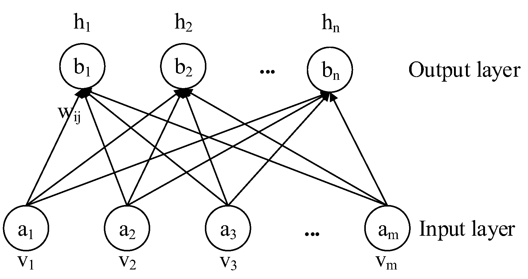
Figure 2.
Schematic representation of a deep belief network (DBN). The number of layers and nodes of each layer are an example; they can be defined as needed.
Figure 2.
Schematic representation of a deep belief network (DBN). The number of layers and nodes of each layer are an example; they can be defined as needed.
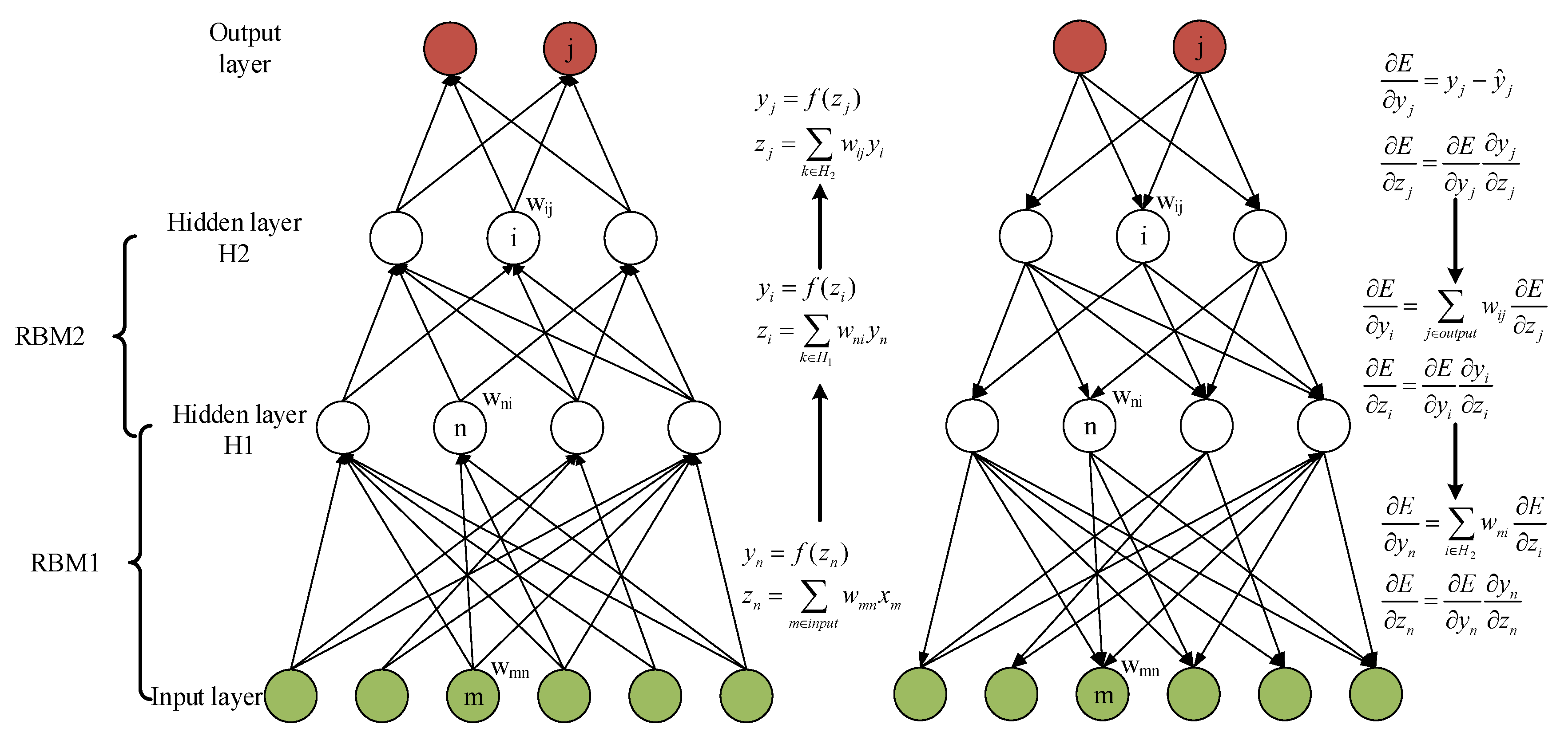
Figure 3.
DBN algorithm flowchart.

Figure 4.
The Fisher discriminative fidelity constraint of a dictionary: in (a) satisfies the structured dictionary well representing . in (b) is the optimal subdictionary in in representing . should have nearly zero coefficients in (c) so that representation are small enough.
Figure 4.
The Fisher discriminative fidelity constraint of a dictionary: in (a) satisfies the structured dictionary well representing . in (b) is the optimal subdictionary in in representing . should have nearly zero coefficients in (c) so that representation are small enough.

Figure 5.
Tennessee Eastman (TE) process flowchart.
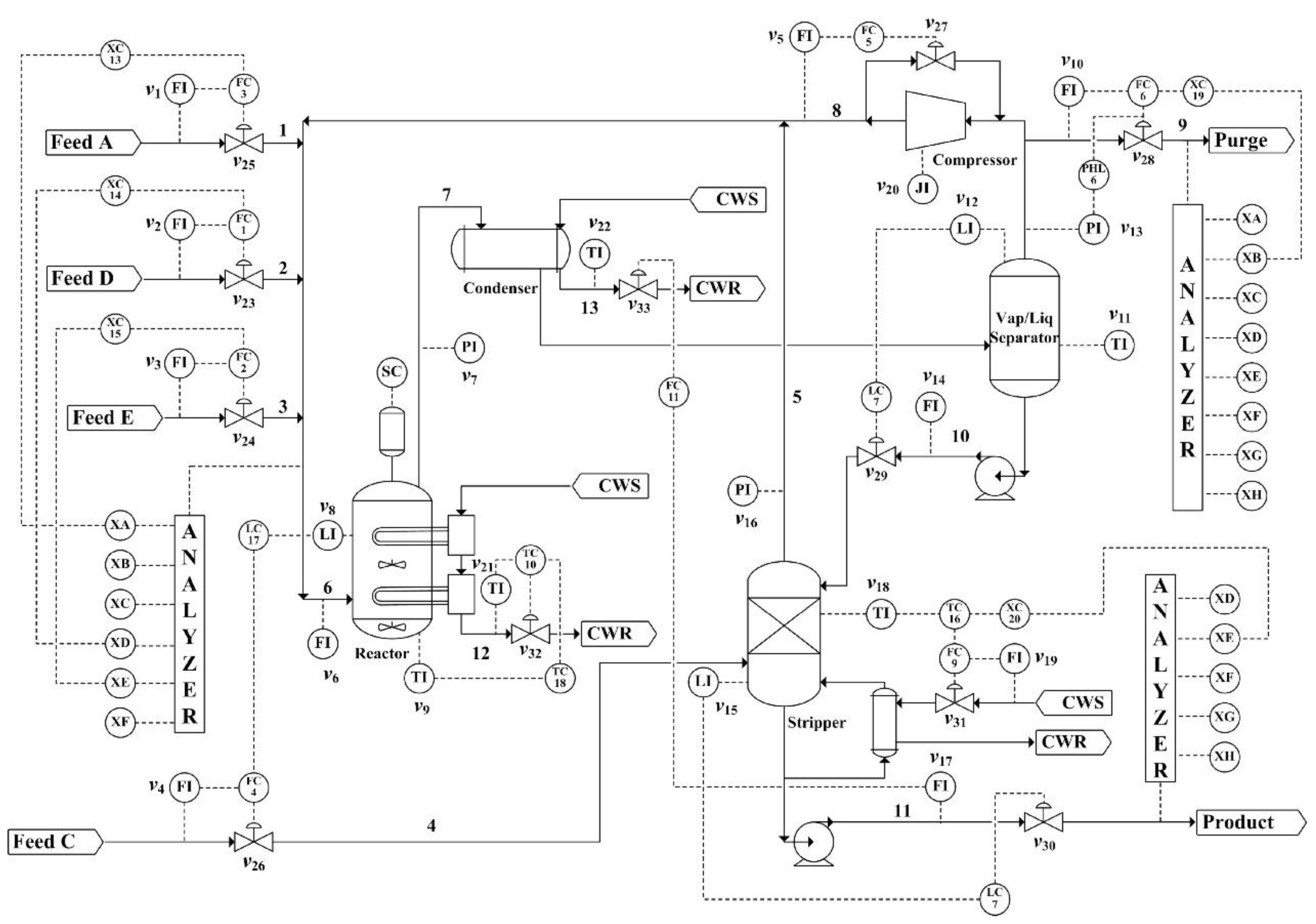
Figure 6.
The deep belief network-Fischer discriminative sparse representation (DBN-FDSR) algorithm.
Figure 6.
The deep belief network-Fischer discriminative sparse representation (DBN-FDSR) algorithm.
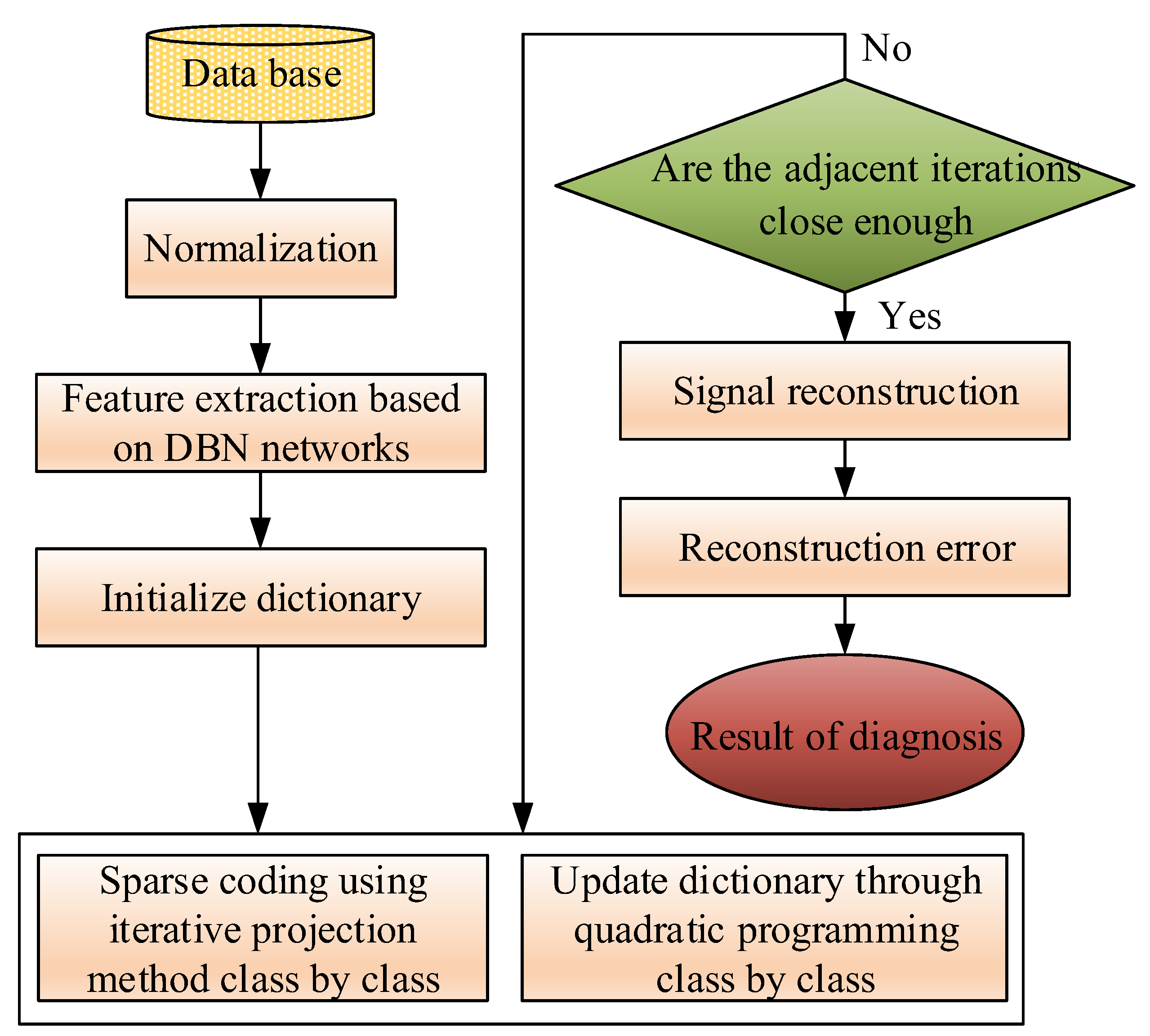
Figure 7.
Visualization of weight vectors of RBM1 and RBM2.

Figure 8.
Visualization of features extracted by DBN ((a) is the view at an azimuth of −37.5 degrees and a top view of 30 degrees, and (b) is the 3D view at an azimuth of 90 degrees and a top view of 90 degrees).
Figure 8.
Visualization of features extracted by DBN ((a) is the view at an azimuth of −37.5 degrees and a top view of 30 degrees, and (b) is the 3D view at an azimuth of 90 degrees and a top view of 90 degrees).
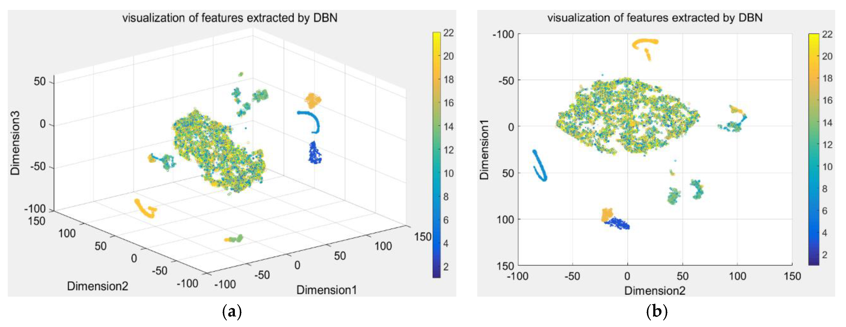
Figure 9.
Visualization of raw data ((a) is the view at an azimuth of −37.5 degrees and a top view of 30 degrees, and (b) is the 3D view at an azimuth of 90 degrees and a top view of 90 degrees).
Figure 9.
Visualization of raw data ((a) is the view at an azimuth of −37.5 degrees and a top view of 30 degrees, and (b) is the 3D view at an azimuth of 90 degrees and a top view of 90 degrees).
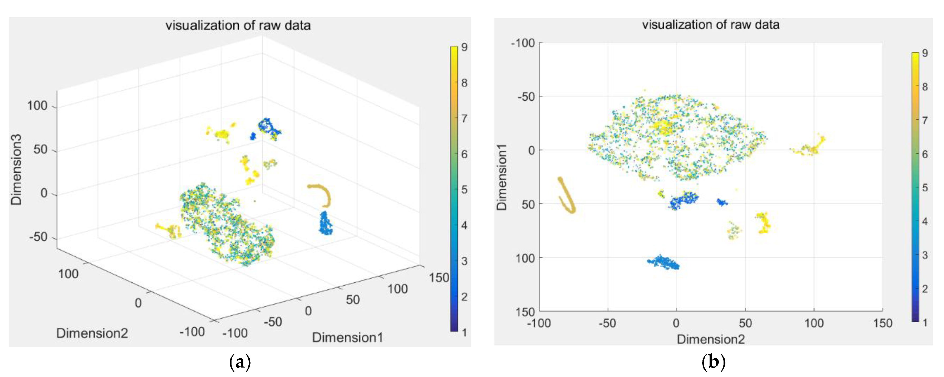
Figure 10.
Visualization of FDSR algorithm result ((a) is the view at an azimuth of −37.5 degrees and a top view of 30 degrees, and (b) is the 3D view at an azimuth of 90 degrees and a top view of 90 degrees).
Figure 10.
Visualization of FDSR algorithm result ((a) is the view at an azimuth of −37.5 degrees and a top view of 30 degrees, and (b) is the 3D view at an azimuth of 90 degrees and a top view of 90 degrees).

Table 1.
Fisher discrimination sparse representation algorithm.
| Input: signal y Initialization: Initialize We initialized using a simple principle component analysis of and ensuring every column of is a unit vector. Step 1: Update the sparse coefficients . Fix and solve one at a time by solving Equation (14). Step 2: Update the dictionary . Fix and solve class by class by solving Equation (15). Step 3: Repeat Steps 1 and 2 until the maximum number of iterations is reached, or the values of adjacent iterations are sufficiently close. Output: Optimal dictionary and sparse coefficient . |
Table 2.
Manipulated and continuously monitored variables.
| Variable Name | Symbol | Variable Name | Symbol |
|---|---|---|---|
| D feed rate | XMV1 | Reactor feed rate | XMEAS6 |
| E feed rate | XMV2 | Reactor pressure | XMEAS7 |
| A feed rate | XMV3 | Reactor level | XMEAS8 |
| A and C feed rate | XMV4 | Reactor temperature | XMEAS9 |
| Recycle compressor | XMV5 | Purge rate | XMEAS10 |
| Purge valve | XMV6 | Separator temperature | XMEAS11 |
| Separator liquid flow | XMV7 | Separator level | XMEAS12 |
| Stripper liquid flow | XMV8 | Separator pressure | XMEAS13 |
| Steam valve of stripper | XMV9 | Separator underflow | XMEAS14 |
| Water flow in reactor | XMV10 | Stripper level | XMEAS15 |
| Water low in condenser | XMV11 | Stripper pressure | XMEAS16 |
| Agitation speed | XMV12 | Stripper underflow | XMEAS17 |
| D feed ratio | XMEAS1 | Stripper temperature | XMEAS18 |
| E feed ratio | XMEAS2 | Stripper steam flow | XMEAS19 |
| A feed ratio | XMEAS3 | Compressor power | XMEAS20 |
| A and C feed ratio | XMEAS4 | Reactor cooling water outlet temperature | XMEAS21 |
| Recycle flow | XMEAS5 | Condenser cooling water outlet temperature | XMEAS22 |
Table 3.
Disturbances in the Tennessee Eastman process.
| Number | Disturb | Type |
|---|---|---|
| 1 | A/D feed ratio changes, B composition constant | Step |
| 2 | B feed ratio changes, A/D composition constant | Step |
| 3 | D feed temperature changes | Step |
| 4 | Reactor cooling water inlet temperature changes | Step |
| 5 | Separator cooling water inlet temperature changes | Step |
| 6 | A feed loss | Step |
| 7 | C head pressure loss | Step |
| 8 | A/B/C composition changes | Random |
| 9 | D feed temperature changes | Random |
| 10 | C feed temperature changes | Random |
| 11 | Reactor cooling water inlet temperature changes | Random |
| 12 | Separator cooling water inlet temperature changes | Slow drift |
| 13 | Reactor dynamic constants changes | Slow drift |
| 14 | Reactor valve | Sticking |
| 15 | Separator valve | Sticking |
| 16 | Unknown | Unknown |
| 17 | Unknown | Unknown |
| 18 | Unknown | Unknown |
| 19 | Unknown | Unknown |
| 20 | Unknown | Unknown |
| 21 | Stable valve in stream 4 | Constant |
Table 4.
Comprehensive comparison of classifier performance.
| Classifier | Normal (%) | Fault 1 (%) | Fault 2 (%) | Fault 6 (%) | Fault 8 (%) | Fault 12 (%) | Fault 13 (%) | Fault 14 (%) | Fault 18 (%) |
|---|---|---|---|---|---|---|---|---|---|
| DBN | 63.2 | 71.0 | 82.7 | 83.0 | 76.5 | 71.4 | 62.0 | 63.4 | 62.0 |
| BP | 81.2 | 83.2 | 76.5 | 75.2 | 77.2 | 64.5 | 65.8 | 66.6 | 63.2 |
| DBN+SVM | 88.1 | 80.1 | 86.5 | 84.2 | 88.2 | 83.1 | 78.2 | 69.2 | 72.0 |
| DBN+SRC | 79.2 | 82.1 | 75.8 | 83.2 | 72.5 | 76.5 | 71.2 | 73.9 | 65.3 |
| DBN+FDSR | 99.2 | 98.2 | 96.5 | 97.8 | 96.8 | 98.9 | 99.3 | 92.3 | 94.5 |
© 2018 by the authors. Licensee MDPI, Basel, Switzerland. This article is an open access article distributed under the terms and conditions of the Creative Commons Attribution (CC BY) license (http://creativecommons.org/licenses/by/4.0/).
Share and Cite
MDPI and ACS Style
Tang, Q.; Chai, Y.; Qu, J.; Ren, H. Fisher Discriminative Sparse Representation Based on DBN for Fault Diagnosis of Complex System. Appl. Sci. 2018, 8, 795. https://doi.org/10.3390/app8050795
AMA Style
Tang Q, Chai Y, Qu J, Ren H. Fisher Discriminative Sparse Representation Based on DBN for Fault Diagnosis of Complex System. Applied Sciences. 2018; 8(5):795. https://doi.org/10.3390/app8050795
Chicago/Turabian StyleTang, Qiu, Yi Chai, Jianfeng Qu, and Hao Ren. 2018. "Fisher Discriminative Sparse Representation Based on DBN for Fault Diagnosis of Complex System" Applied Sciences 8, no. 5: 795. https://doi.org/10.3390/app8050795
Note that from the first issue of 2016, this journal uses article numbers instead of page numbers. See further details here.