Fault-Tolerant Control Strategy of a Wind Energy Conversion System Considering Multiple Fault Reconstruction

Key Laboratory of Advanced Process Control for Light Industry, Jiangnan University, Wuxi 214122, China
*
Author to whom correspondence should be addressed.
Appl. Sci. 2018, 8(5), 794; https://doi.org/10.3390/app8050794
Submission received: 27 March 2018
/
Revised: 11 May 2018
/
Accepted: 11 May 2018
/
Published: 16 May 2018
(This article belongs to the Section Mechanical Engineering)
Abstract
:A robust sliding mode observer (SMO) is proposed to achieve multiple fault reconstruction for a wind energy conversion system (WECS) with simultaneous actuator and sensor faults. Firstly, the state equation of the WECS is established. The orthogonal transformation matrix and a post filter are introduced, and a new augmented system is constructed; then, the sensor fault is converted into an actuator fault to diagnose. The fault information is collected by the equivalent output control, and the simultaneous reconstruction algorithm of the sensor fault and the actuator fault is given. Through compensation control, the reliable control input of the WECS is guaranteed, and the function of active fault tolerant control for multiple faults is achieved. Simulation experiments show that the proposed method can accurately reconstruct the actuator and sensor faults, and maximum wind energy capture can be achieved by active fault-tolerant control.
1. Introduction
Wind power generation is the most mature, largest and most promising power generation method for new energy [1]. Wind power plants are generally located in complex terrain and bad climates. The WECS, an important part of the wind power generation system, has a high fault rate, especially in its sensor and actuator, which seriously affect the performance of the system, even causing system paralysis, and cause immeasurable losses [2]. Therefore, realizing the fault tolerant control of WECS is an important guarantee for improving the operation reliability of wind power generation systems.
Fault-tolerant control aims to ensure a stable and safe operation of the controlled system under the requirements of a certain performance index when it fails [3]. Passive fault-tolerant control strategy cannot control the unknown faults of the system, while active fault tolerance can redesign the controller by using a priori knowledge of all kinds of faults [4]. Active fault-tolerant control is applied to various practical projects. An active fault-tolerant tracking controller is proposed for vehicle dynamics systems in [5], and the uncertain dynamic model of the vehicle is established. the vehicle dynamic states with sensor faults are estimated by the description observed and a fault-tolerant tracking controller based on linear matrix inequalities is designed. A robust output-feedback control strategy applied to the path following an autonomous ground vehicle is presented in [6], and a robust static output-feedback controller based on mixed genetic algorithms/linear matrix inequality is used to realize the path-following without the information of the lateral velocity. Active fault-tolerant control has also been widely studied and applied in WECS. An adaptive fault observer is designed for WECS, which detects the faults of the transmission part of the conversion system, and an active fault tolerant controller is designed to ensure the reliable and stable operation of the system [7]. An active tolerant controller based on is designed to obtain the high performance in extreme wind speed profile, and a sliding mode fault detection and isolation system is applied to reconstruct and compensate a wind turbine’s sensor faults in [8].
The T-S fuzzy model proposed by Takagi T etc. is an effective method to solve the problem of nonlinear system control [9]. A proportional integral observer based on T-S fuzzy control is designed for the fault estimation of the actuator and sensor in [10]. Through the Lyapunov stability theory and performance analysis, the sufficient design conditions for simultaneous estimation of two kinds of faults are given, and the proposed conditions are solved under linear matrix inequalities constraints and the proportional integral observer gains are calculated. Aiming at the potential faults of the system, fuzzy modeling and the recognition method are used to automatically correct the potential faults of the system based on online diagnosis information, so as to ensure that the motor torque can be reliably adjusted when the actuator fails [11]. A multi-observer scheme based on Calman filter and maximum shift strategy is presented for the additive and multiplicative faults of sensors, and the fault types are diagnosed by generating new residual values in [12].
Sliding mode control can effectively deal with the uncertainty and interference of complex dynamic systems and adjust the dynamic behavior of the system by selecting sliding function [13] so that the nonlinear system has strong robustness, and this is widely applied in engineering practice, such as CNC machine tools [14], four-rotor helicopters [15], wind turbines [16] and so on. In [17], a two-order sliding mode is designed for the parameter variable and external disturbance of the wind energy system based on doubly-fed induction generators DFIG, and the variable structure control based on the two-order derivative of the a properly chosen sliding manifold is designed to further improve the performance of the system. In [18], a class of MIMO (multiple-input multiple-output) nonlinear system’s derivative and integral terminal sliding mode control is proposed to realize the limited convergence time of the more general high order MIMO system and avoid the singular problems in the design of the controller. Fault detection and isolation for induction generators based on a sliding mode observer is proposed in [19] by means of maximum power point tracking, and the induction generator closed loop via indirect rotor flux-oriented control is described. The WECS has the characteristics of being nonlinear, having strong coupling, being multivariable and so on, and is seriously disturbed by external interference. Through the sliding mode control, the WECS has strong robustness and excellent insensitivity to faults and external interference.
The WECS is usually composed of a wind turbine, transmission link, generator, Alternating Current-Direct Current (AC-DC) converter and so on; there has been much research on fault diagnosis and fault-tolerant control of different links in the WECS. A Wound Rotor Induction Generator (WRIG)-based wind energy system associated with hybrid AC/DC microgrid (DCM) is introduced in [20], which runs under an islanded and utility-tied mode. The system operation and power transfer under the islanded and utility-tied mode are realized at all possible conditions, and the effectiveness of the system in the process of load changes is proved by the dynamic experimental results of various modes. For MPP (maximum power point) and no-MPP tracking operations, two different methods, the difference between the actual and simulated output power of the wind system and the predetermined angular shaft speed ratio are adopted respectively as indictors to detect the lubricant system faults in [21]. According to different operation modes, different diagnostic criteria are used to diagnose faults; although it is helpful for better detection of faults, the process design is rather complicated. An active fault-tolerant fuzzy control strategy based on multi observer switching control is proposed in [22], the T-S fuzzy modeling of WECS is carried out and sufficient conditions for robust stabilization of system are given by deriving Taylor series and linear matrix inequalities. Multi-observer switching control leads to an increase in the number of constraints, which is limited in engineering applications, and the actuator fault is not considered in it. A fault diagnosis method for the lubrication system and the converter in the wind energy system is presented in [23], and the tolerance of the supervisory controller towards a lubrication system and converter fault in the wind system is explained to satisfy the demanded power with maximum utilization. Compared with proposed robust formulation, this paper has been optimized to better solve the uncertainty of the WECS. With the increase of the scale of WECS, the number of actuators and sensors is increasing, and the probability of simultaneous faults is increasing. Previous works focused on fault diagnosis and fault tolerant control of a single actuator or sensor. Therefore, it is more practical to study the multi-fault diagnosis of WECS.
In this paper, the state equation of the WECS is established in the case of the simultaneous faults of the actuator and the sensor in the WECS. Based on the SMO, a new augmented system is constructed by introducing the orthogonal transformation matrix and constructing the post filter. The sensor fault is converted into the actuator fault to diagnose, and a robust adaptive fault reconstruction observer is designed to achieve multiple fault reconstruction. A robust fault-tolerant controller for WECS is designed to guarantee the reliable control input of the WECS and to capture the maximum wind energy. The simulation results are given to verify the superiority of the proposed method.
2. Mathematical Modeling of WECS Based on DFIG
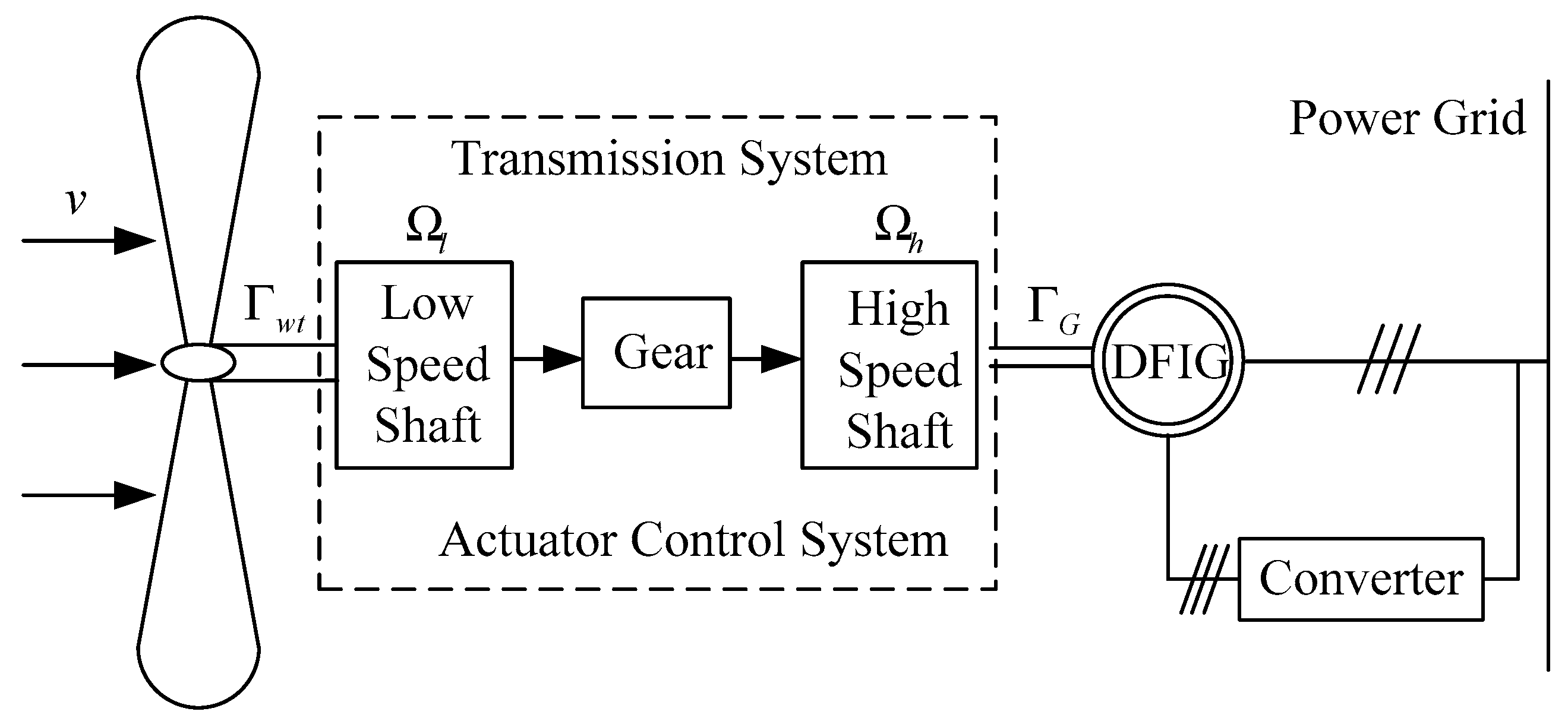
Doubly-fed induction generators (DFIG) are widely used in wind power systems due to their stability, robustness and relatively low cost. As a result, the doubly fed wind power generation system is taken as an example [24]—WECS based on DFIG—as shown in Figure 1. The wind power is converted to mechanical energy by a wind turbine, and the DFIG is driven by the drive system to generate electric energy and then transmitted to the power grid through an AC-DC converter.
Assuming that the wind turbine is an ideal state, according to Baez theory, the mechanical power of the wind turbine is as follows [25]:
The wind torque produced by the wind turbine is as follows [26]:
where is the air density, is the wind speed, is the blade length, is the conversion coefficient of wind energy. is the ratio of blade tip velocity to wind speed; that is, , is the angular velocity of wind turbine rotor(low speed shaft), and is the torque coefficient, satisfying .
In order to simplify the modeling, the rigid model is adopted in the connection between the high-speed axis and the low speed axis [27]; the equation of motion of the transmission system Equations (3) and (4) is as follows:
where is the rotor speed (high speed shaft) of generator, that is, , is the gear transmission ratio, is the electromagnetic torque of generator, is the transmission efficiency, is the high speed shaft inertia, is the low speed shaft inertia.
Some dynamic characteristics of the model are neglected and, considering that the electromagnetic time constant is much smaller than the mechanical time constant, the dynamic process of electromagnetic response of generator is ignored when modeling the system [28]. The state equation of WECS is modeled as follows:
where , , , , ; is the state vector, is the input vector, is the output vector, is the reference value of the electromagnetic torque of the generator, and is the electromagnetic time constant [29].
3. Sensor Fault Conversion
The faults of WECS include system faults, actuator faults, sensor faults and so on. Actuator faults usually occur due to wear and destruction of gears in gear boxes, and wear and deformation of bearing surfaces. Sensors usually fail due to their aging damage and uncorrected long-term use. Considering the faults of the WECS, the system (5) can be described as
where , , , , , , and are full rank matrixes, is the actuator fault, is the sensor fault, is the actuator fault distribution matrix, and is the sensor fault distribution matrix.
Assumption 1.
andare norm bounded.
Assumption 2.
System Equation (6) satisfies.
Assumption 3.
.
Based on system Equation (6), the orthogonal matrix is introduced [30] and can be obtained as follows:
State variable Equation (8) is defined as follows:
where is the state variable of by the filter, is a nonsingular matrix, is designed to filter the matrix, and Equations (7) and (8) are brought into the Equation (6), and the new system equation is obtained:
Equation (9) is simplified and the new state variables and the system matrices are defined as follows: , , , , , , .
Equation (9) can be transformed into:
Equation (10) is a system with an actuator fault and sensor fault , which is equivalent to actuator faults in Equation (6).
4. Design and Reconstruction of Sliding Mode Fault Observer (SMFRO)
4.1. Design of Robust Adaptive Sliding Mode Fault Observer
For the system Equation (10), the sliding mode state observer is designed as follows:
where is the undetermined gain matrix, is the nonlinear feedback matrix, and is the sliding mode strategy to be designed. The state estimation error of the observer is defined as , the output estimation error is , and the deviation system equation is obtained by Equations (10) and (12).
According to the system Equation (11), a sliding mode fault reconstruction observer is proposed:
where is the arbitrary stable matrix, the robust SMO is undetermined gain matrix and the nonlinear feedback matrix is, respectively, , .
It is assumed that the deviation between the system (10) and the SMO (12) is always bounded: , is the normal number, and the following sliding mode strategy is proposed for the observer Equation (12):
where is the Lyapunov matrix of , is the correction coefficient and .
The state estimation error is , and the output deviation is . The state and output equations of the system are Equations (15) and (16):
According to [32], the system Equations (15) and (16) are asymptotically stable. When , the SMO is asymptotically stable.
4.2. Robust Multiple Fault Reconstruction
The discontinuous switch , i.e., sliding mode strategy Equation (14), makes the observer deviation equation produce a sliding mode motion to ensure the robustness of the system to the external disturbance, but it will inevitably produce chattering and bring high frequency interference to the system. When the sliding mode motion reaches ; i.e., , where is the equivalent output control. Because has a stable pole, it makes , then . In order to reduce the chattering phenomenon, the continuous function approximation method is used to approximate the sliding mode and Equation (17) is obtained [33]:
where is the normal number with less accuracy. The equivalent output control Equation (17) makes the reconfiguration system robust, and the robust fault reconstruction expression is as follows:
The robust fault reconstruction expressions for the actuator and the sensor are Equations (19) and (20):
5. Design and Reconstruction of Sliding Mode Fault Observer (SMFRO)
A sliding surface expression Equation (21) is designed for WECS:
where is the time constant of the convergent speed of sliding mode control, that is, , then . A stable sliding surface can be obtained by the Equation (21). The sliding mode control law consists of the equivalent control input and the switch part two parts are as follow [29]:
where , , is the derivative of the power coefficient , and is the hysteresis function of the bandwidth of .
The multi fault reconstruction block diagram of the WECS is shown in Figure 2.
The fault output of the sliding mode controller is as follows:
The output of the sliding mode fault reconstruction observer is as follows:
The control input of the WECS is obtained by the Equations (25) and (26).
6. Experiments and Results
A three-lobe horizontal axis doubly fed wind energy conversion system with low power (6 kw), high speed and fixed pitch is used [30]. The simulation is carried out by Matlab software. The simulation parameters are shown in Table 1 as follows:
Under the rated wind speed [27], the fixed pitch control is adopted, i.e., , and the wind energy conversion coefficient is determined by Equation (28):
In the case of a certain wind speed, when the blade tip speed ratio is , the maximum value is 0.476: the best tip speed ratio.
The wind speed of the WECS is shown in Figure 3.
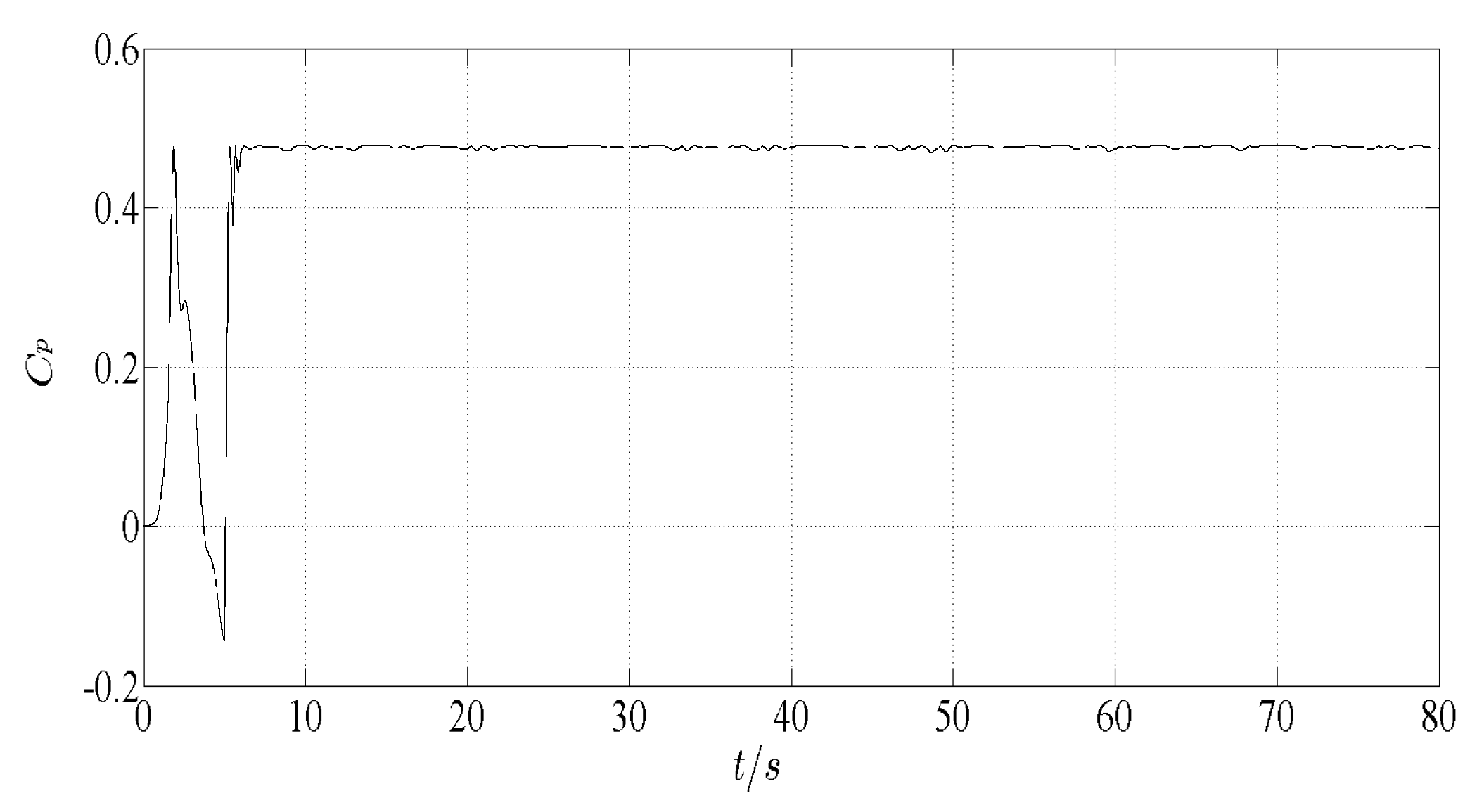
When there are no faults in the WECS, the reference value of the electromagnetic torque is , and the wind energy conversion coefficient is , as shown in Figure 4 and Figure 5.
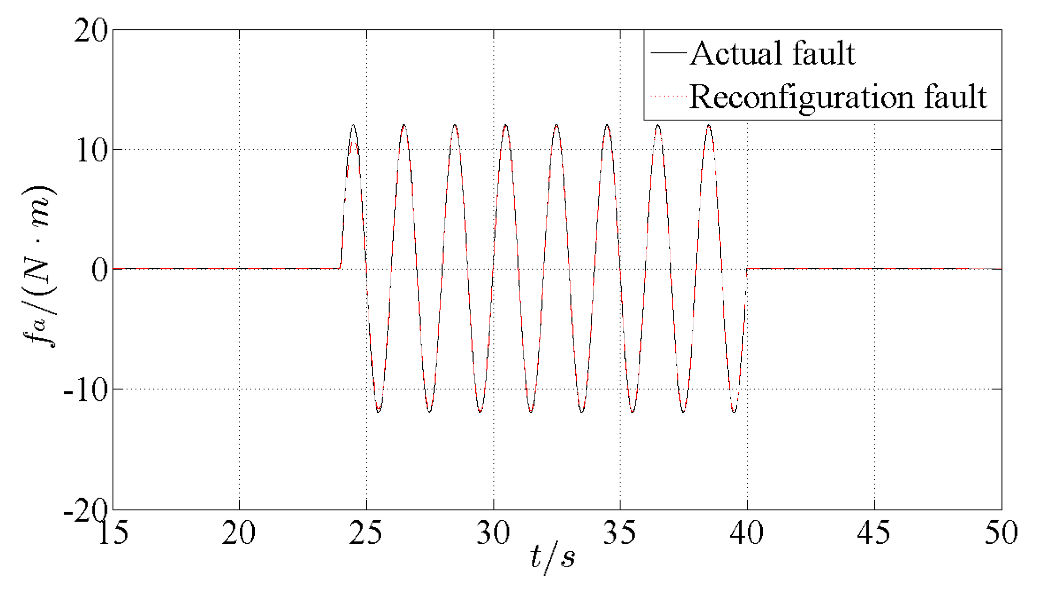
When the wind energy conversion system fails, the expression of the actuator fault is as follows:
The fault time is set to .
The expression of sensor fault is
The fault time is set to .
The proposed fault reconstruction algorithm is used to reconstruct the actuator fault. The reconfiguration of actuator fault is shown in Figure 6 and the reconfiguration of sensor fault is shown in Figure 7. In the range of error allowed, the online tracking and reconfiguration of the fault can be realized.
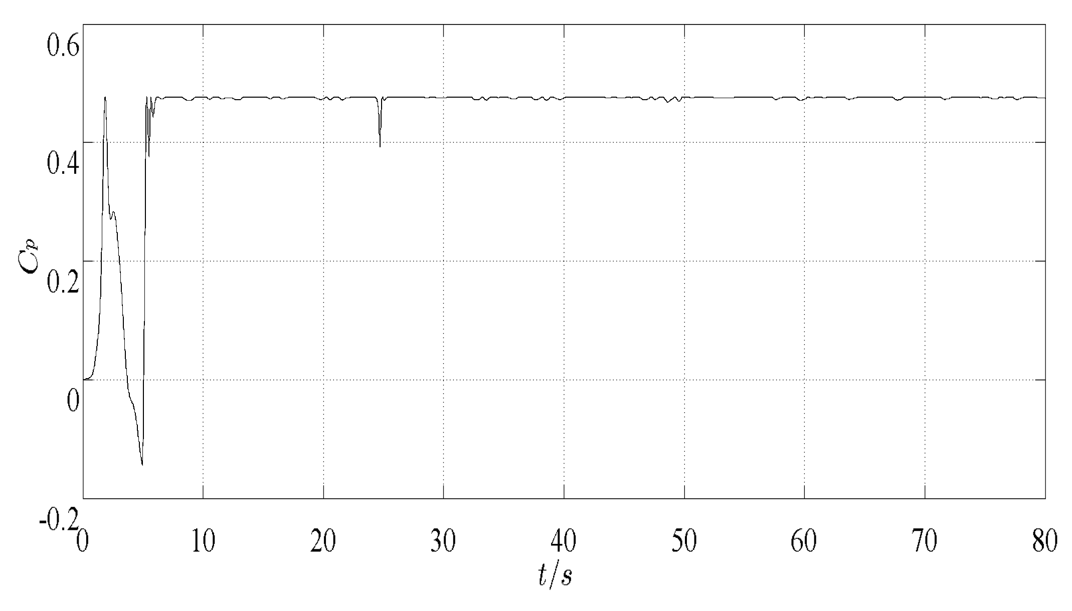
When the actuator fault Equation (30) and the sensor fault occurs, the electromagnetic torque reference value and the wind energy conversion coefficient are shown in Figure 8 and Figure 9, respectively.
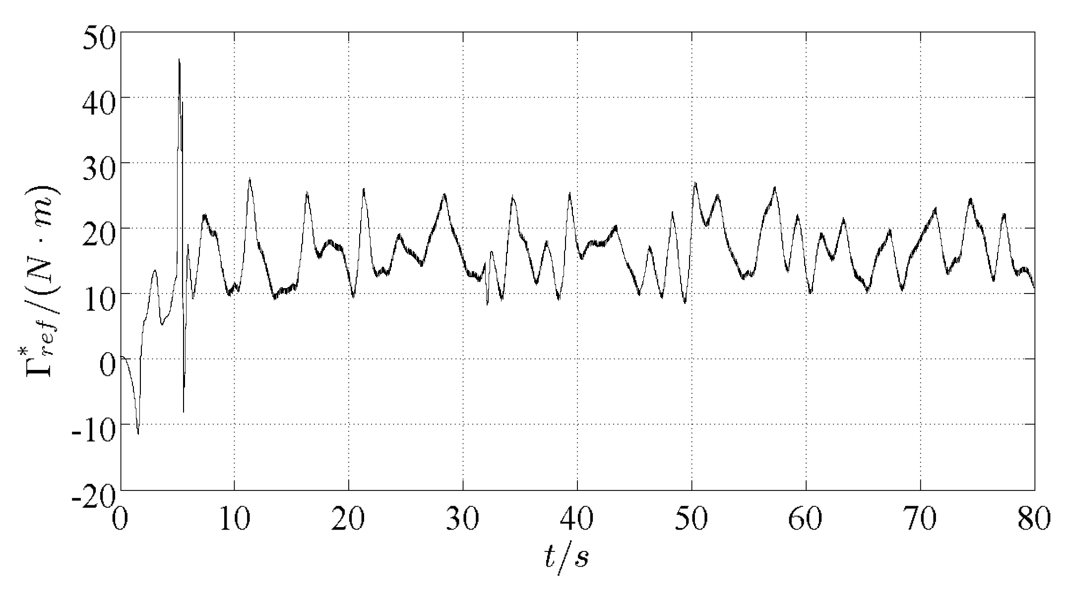
When the fault occurs, the wind energy conversion coefficient varies greatly, which affects the capture of wind energy. After adopting an active fault-tolerant controller, the capture efficiency is significantly improved and the purpose of optimization is achieved. The reference value of electromagnetic torque and wind energy conversion coefficient after fault-tolerant control are shown in Figure 10 and Figure 11. Compared with Figure 8 and Figure 9 and Figure 10 and Figure 11, the expected value of the wind energy conversion coefficient is reached and the maximum wind energy capture is achieved after active fault tolerance control.
7. Conclusions
In this paper, the problem of system fault reconstruction and fault-tolerant control is discussed when multiple faults occur in the WECS. Firstly, the state equation of the WECS is established. Based on the SMO, a new augmented system is constructed by orthogonal transformation matrix and post filter, and the sensor fault is converted into the actuator fault to diagnose. A robust adaptive SMO is designed, and an optimized sliding mode strategy is given to ensure the stability of the state estimation of the system. The fault information is collected in real time by the equivalent output control, and the simultaneous reconstruction algorithm of the sensor fault and the actuator fault is given. Finally, a robust fault-tolerant controller is designed to ensure reliable control input of the WECS. When sensor and actuator faults occur, fault-tolerant control can be carried out successfully to achieve maximum wind energy capture.
Author Contributions
X.W. conceived the experiment and wrote the paper; Y.S. helped in the experiment and writing.
Acknowledgments
This work was supported in part by the National Nature Science Foundation under Grant 61573167 and grant 61572237, in part by the Postgraduate Research and Practice Innovation Program of Jiangsu Province under Grant KYCX17_1488.
Conflicts of Interest
The authors declare no conflict of interest.
References
- Xu, J.; Li, L.; Zheng, B. Wind energy generation technological paradigm diffusion. Renew. Sustain. Energy Rev. 2016, 59, 436–449. [Google Scholar] [CrossRef]
- Sun, X.; Huang, D. An Explosive Growth of Wind Power in China. Int. J. Green Energy 2014, 11, 849–860. [Google Scholar] [CrossRef]
- Kamal, E.; Aitouche, A.; Ghorbani, R.; Bayart, M. Fuzzy Scheduler Fault-Tolerant Control for Wind Energy Conversion Systems. IEEE Trans. Control Syst. Technol. 2013, 22, 119–131. [Google Scholar] [CrossRef]
- Shi, F.; Patton, R. An active fault tolerant control approach to an offshore wind turbine model. Renew. Energy 2015, 75, 788–798. [Google Scholar] [CrossRef]
- Aouaouda, S.; Chadli, M.; Boukhnifer, M.; Karimi, H.R. Robust fault tolerant tracking controller design for vehicle dynamics: A descriptor approach. Mechatronics 2015, 30, 316–326. [Google Scholar] [CrossRef]
- Hu, C.; Jing, H.; Wang, R.; Yan, F.; Chadli, M. Robust H∞ output-feedback control for path following of autonomous ground vehicles. Mech. Syst. Signal Process. 2016, 70, 414–427. [Google Scholar] [CrossRef]
- Wu, Z.Q.; Yang, Y.; Xu, C.H. Adaptive fault diagnosis and active tolerant control for wind energy conversion system. Int. J. Control Autom. Syst. 2015, 13, 120–125. [Google Scholar] [CrossRef]
- Saberi, A.; Salmasi, F.R.; Najafabadi, T.A. Sensor fault-tolerant control of wind turbine systems. In Proceedings of the 5th Conference on Thermal Power Plants (CTPP), Tehran, Iran, 10–11 June 2014; pp. 40–45. [Google Scholar]
- Takagi, T.; Sugeno, M. Fuzzy identification of systems and its applications to modeling and control. Read. Fuzzy Sets Intell. Syst. 1993, 15, 387–403. [Google Scholar]
- Youssef, T.; Chadli, M.; Karimi, H.R.; Wang, R. Actuator and sensor faults estimation based on proportional integral observer for T-S fuzzy model. J. Frankl. Inst. 2016, 354, 2524–2542. [Google Scholar] [CrossRef]
- Badihi, H.; Zhang, Y.; Hong, H. Wind Turbine Fault Diagnosis and Fault-Tolerant Torque Load Control Against Actuator Faults. IEEE Trans. Control Syst. Technol. 2015, 23, 1351–1372. [Google Scholar] [CrossRef]
- Beddek, K.; Merabet, A.; Kesraoui, M.; Tanvir, A.A.; Beguenane, R. Signal-Based Sensor Fault Detection and Isolation for PMSG in Wind Energy Conversion Systems. IEEE Tran. Instrum. Meas. 2017, 66. [Google Scholar] [CrossRef]
- Shtessel, Y.; Edwards, C.; Fridman, L.; Levant, A. Sliding Mode Control and Observation; Birkhäuser: New York, NY, USA, 2014. [Google Scholar]
- Zhao, P.; Shi, Y.; Huang, J. Proportional-integral based fuzzy sliding mode control of the milling head. Control Eng. Pract. 2016, 53, 1–13. [Google Scholar] [CrossRef]
- Jia, Z.; Yu, J.; Mei, Y.; Chen, Y.; Shen, Y.; Ai, X. Integral Backstepping Sliding Mode Control for Quadrotor Helicopter under External Uncertain Disturbances. Aerosp. Sci. Technol. 2017, 68, 299–307. [Google Scholar] [CrossRef]
- Morshed, M.J.; Fekih, A. A comparison study between two sliding mode based controls for voltage sag mitigation in grid connected wind turbines. In Proceedings of the IEEE Conference on Control Applications (CCA), Sydney, Australia, 21–23 September 2015; pp. 1913–1918. [Google Scholar]
- Morshed, M.J.; Fekih, A. Design of a second order Sliding Mode approach for DFIG-based wind energy systems. In Proceedings of the American Control Conference, Seattle, WA, USA, 24–26 May 2017; pp. 729–734. [Google Scholar]
- Chiu, C.S. Derivative and integral terminal sliding mode control for a class of MIMO nonlinear systems. Automatica 2012, 48, 316–326. [Google Scholar] [CrossRef]
- Sellami, T.; Berriri, H.; Jelassi, S.; Darcherif, A.M.; Mimouni, M.F. Sliding Mode Observers-based Fault Detection and Isolation for Wind Turbine-driven Induction Generator. Int. J. Power Electron. Drive Syst. 2017, 8, 1345–1358. [Google Scholar] [CrossRef]
- Sowmmiya, U.; Govindarajan, U. Control and power transfer operation of WRIG-based WECS in a hybrid AC/DC microgrid. IET Renew. Power Gener. 2018, 12, 359–373. [Google Scholar] [CrossRef]
- Hosseinzadeh, M.; Salmasi, F.R. Analysis and detection of a wind system failure in a micro-grid. J. Renew. Sustain. Energy 2016, 8, 043302. [Google Scholar] [CrossRef]
- Kamal, E.; Aitouche, A.; Bayart, M. Fault Tolerant Control of Wind Energy Conversion Systems Subject to Sensor Faults. In Sustainability in Energy and Buildings; Springer: Berlin/Heidelberg, Germany, 2012; pp. 231–241. [Google Scholar]
- Hosseinzadeh, M.; Salmasi, F.R. Fault-Tolerant Supervisory Controller for a Hybrid AC/DC Micro-Grid. IEEE Trans. Smart Grid 2016, 99. [Google Scholar] [CrossRef]
- Fekih, A.; Hmida, J.B.; Morshed, M.J. A feedback linearization control scheme for maximum power generation in wind energy systems. In Proceedings of the 24th Mediterranean Conference on Control and Automation, Athens, Greece, 21–24 June 2016; pp. 275–279. [Google Scholar]
- Sanchez, A.G.; Molina, M.G.; Lede, A.M.R. Dynamic model of wind energy conversion systems with PMSG-based variable-speed wind turbines for power system studies. Int. J. Hydrog. Energy 2012, 37, 10064–10069. [Google Scholar] [CrossRef]
- Kaloi, G.S.; Wang, J.; Baloch, M.H. Dynamic Modeling and Control of DFIG for Wind Energy Conversion System Using Feedback Linearization. J. Electr. Eng. Technol. 2016, 11, 1137–1146. [Google Scholar] [CrossRef]
- Munteanu, I.; Cutululis, N.A.; Bratcu, A.I.; Ceanga, E. Optimal Control of Wind Energy Systems; Springer: London, UK, 2008. [Google Scholar]
- Esbensen, T.; Sloth, C. Fault Diagnosis and Fault-Tolerant Control of Wind Turbines; Aalborg University: Aalborg, Denmark, 2008; pp. 9–23. [Google Scholar]
- Munteanu, I.; Bacha, S.; Bratcu, A.I.; Guiraud, J.; Roye, D. Energy-Reliability Optimization of Wind Energy Conversion Systems by Sliding Mode Control. IEEE Trans. Energy Convers. 2008, 23, 975–985. [Google Scholar] [CrossRef]
- Brahim, A.B.; Dhahri, S.; Hmida, F.B.; Sellami, A. Robust and simultaneous reconstruction of actuator and sensor faults via sliding mode observer. In Proceedings of the International Conference on Electrical Engineering and Software Applications, Hammamet, Tunisia, 21–23 March 2013; pp. 1–6. [Google Scholar]
- Tan, C.P.; Edwards, C. Sliding mode observers for robust detection and reconstruction of actuator and sensor faults. Int. J. Robust Nonlinear Control 2003, 13, 443–463. [Google Scholar] [CrossRef]
- Edwards, C. On the development of discontinuous observers. Int. J. Control 1994, 59, 1211–1229. [Google Scholar] [CrossRef]
- Edwards, C.; Patton, R.J.; Spurgeon, S.K. Sliding mode observers for fault detection and isolation. Automatica 2000, 36, 541–553. [Google Scholar] [CrossRef]
Figure 1.
Wind energy conversion system (WECS) based on doubly-fed induction generators (DFIG).

Figure 2.
Multi fault reconstruction control block diagram of WECS.
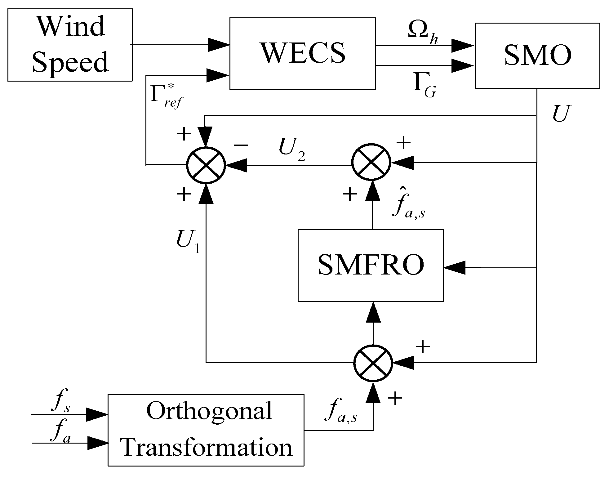
Figure 3.
Wind speed waveform.
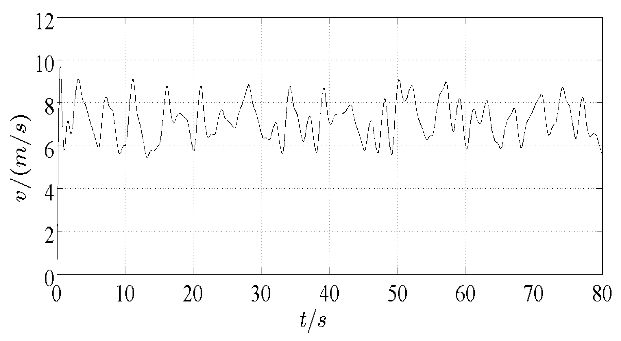
Figure 4.
Reference value of electromagnetic torque without fault .

Figure 5.
Wind energy conversion coefficient without fault.

Figure 6.
Actuator fault and reconfiguration.

Figure 7.
Sensor fault and reconfiguration.
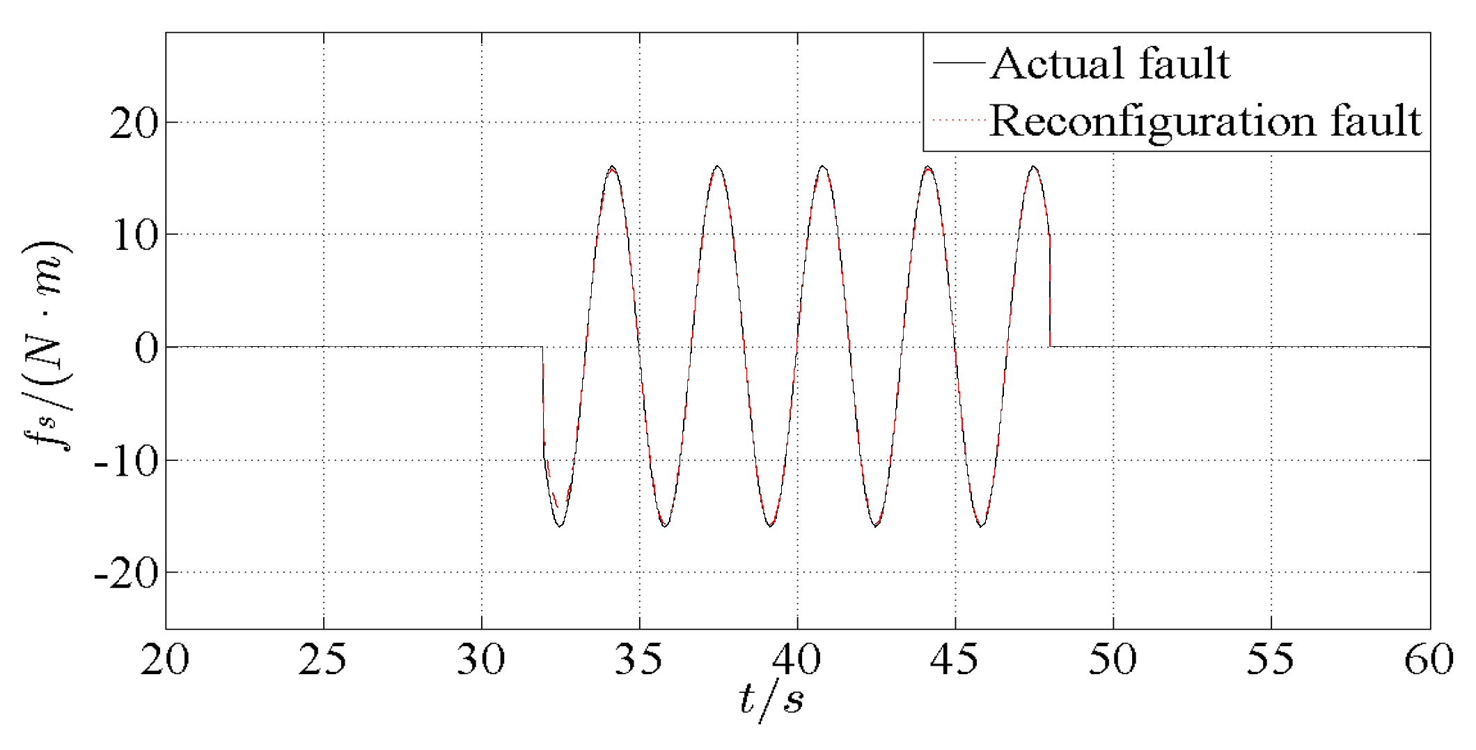
Figure 8.
The reference value of electromagnetic torque at the time of fault.
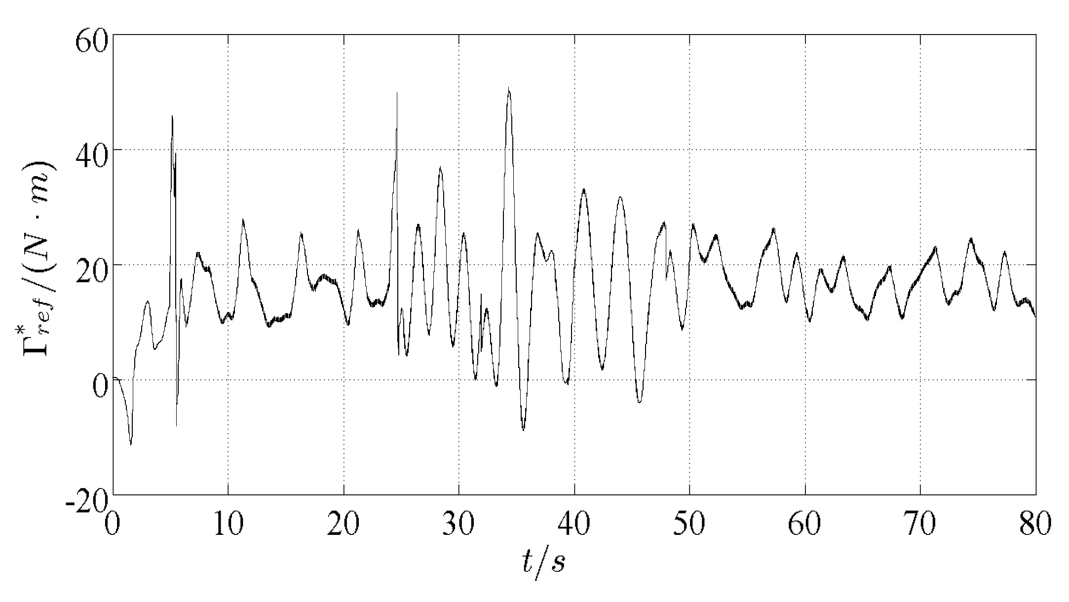
Figure 9.
The wind energy conversion coefficient at the time of fault.
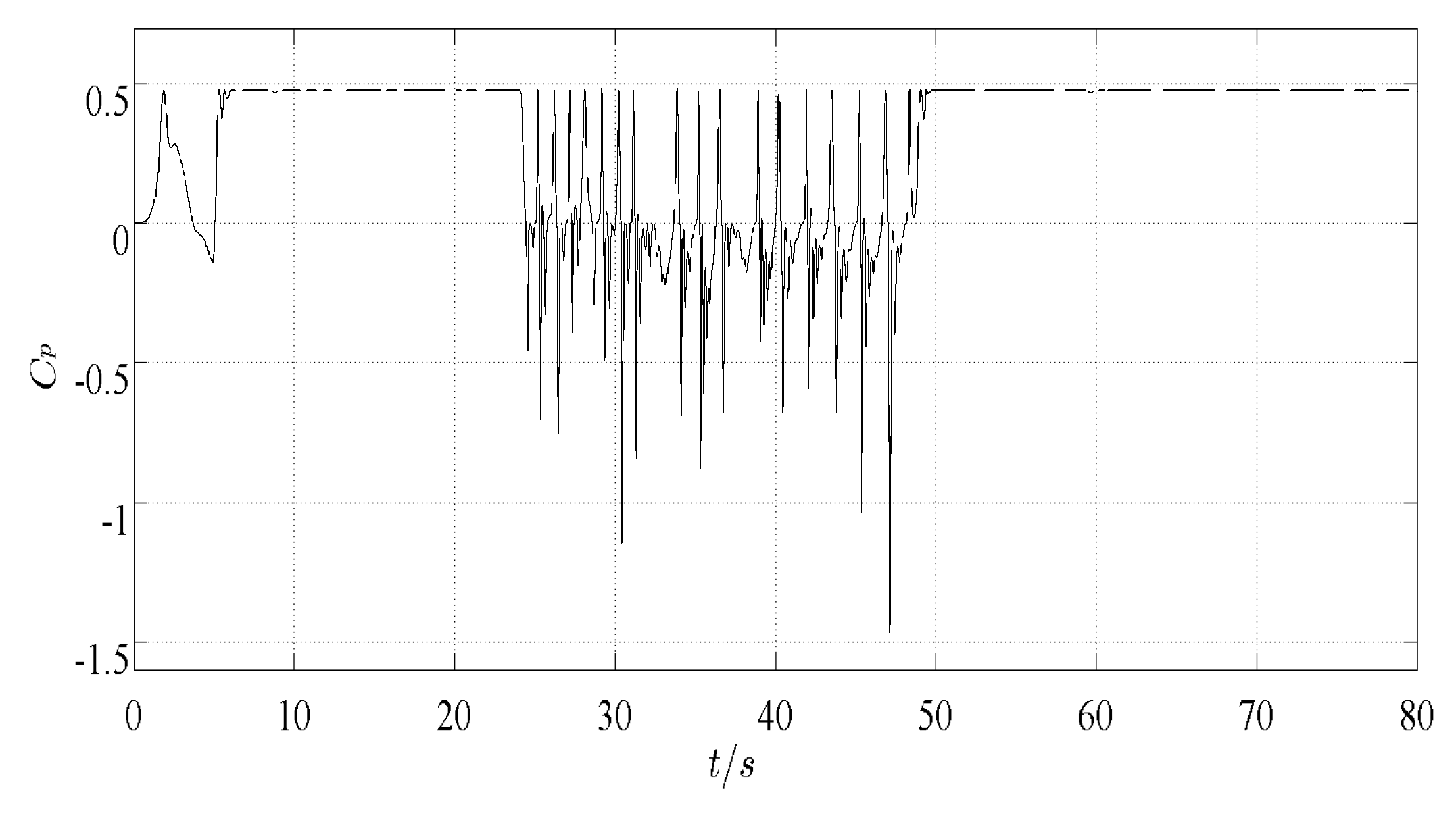
Figure 10.
The reference value of electromagnetic torque after fault-tolerant control.
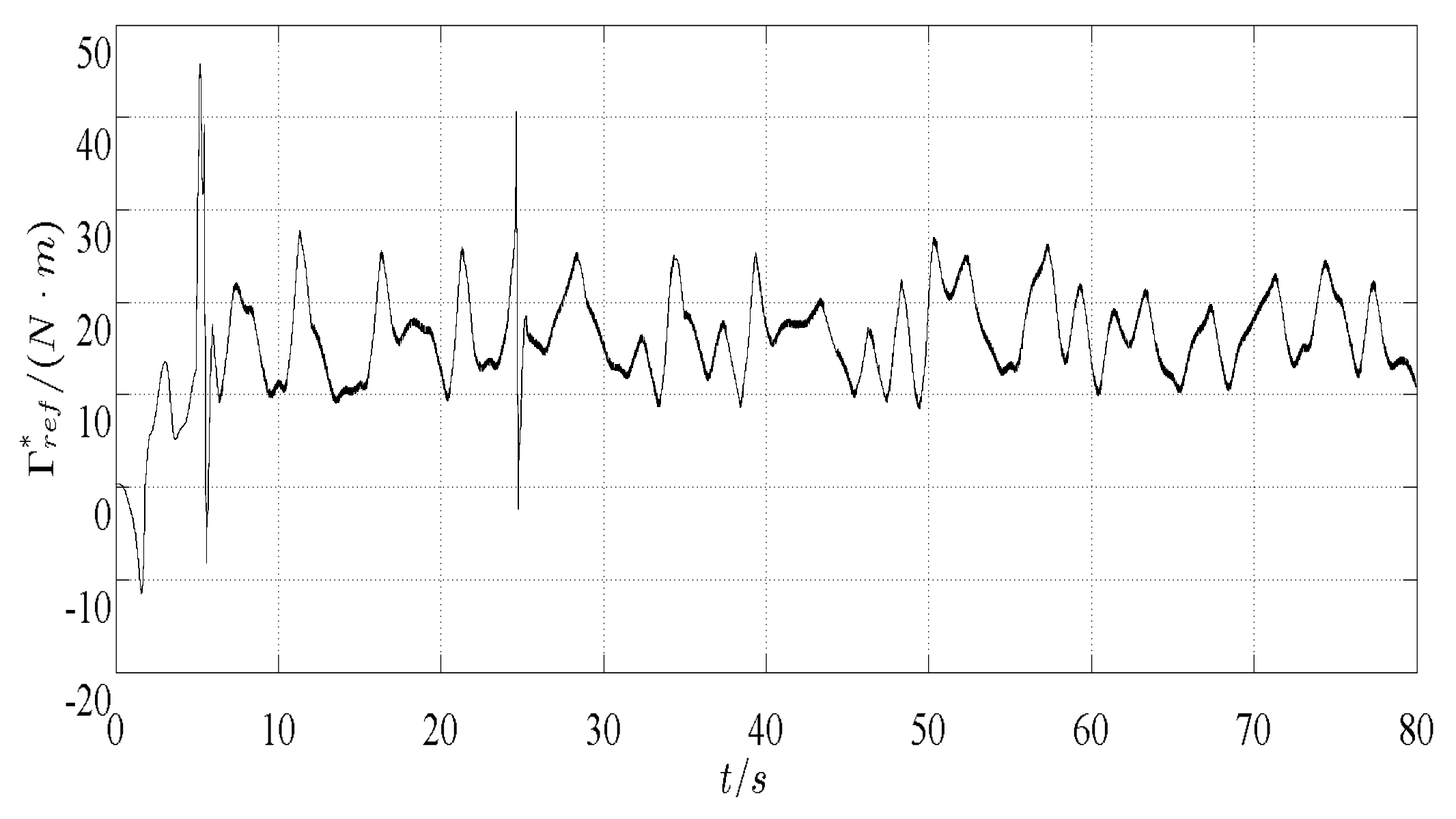
Figure 11.
The wind energy conversion coefficient after fault-tolerant control.


Table 1.
Simulation Parameters.
| Parameter Symbols | Parameter Names | Parameter Values |
|---|---|---|
| Rated voltage | ||
| Rated speed | ||
| Rated electromagnetic torque | ||
| Air density | ||
| Transmission efficiency | ||
| Transmission speed ratio | ||
| Blade length | ||
| Moment of inertia of high speed axis | ||
| Moment of inertia of low speed axis | ||
| Electromagnetic time constant |
© 2018 by the authors. Licensee MDPI, Basel, Switzerland. This article is an open access article distributed under the terms and conditions of the Creative Commons Attribution (CC BY) license (http://creativecommons.org/licenses/by/4.0/).
Share and Cite
MDPI and ACS Style
Wang, X.; Shen, Y. Fault-Tolerant Control Strategy of a Wind Energy Conversion System Considering Multiple Fault Reconstruction. Appl. Sci. 2018, 8, 794. https://doi.org/10.3390/app8050794
AMA Style
Wang X, Shen Y. Fault-Tolerant Control Strategy of a Wind Energy Conversion System Considering Multiple Fault Reconstruction. Applied Sciences. 2018; 8(5):794. https://doi.org/10.3390/app8050794
Chicago/Turabian StyleWang, Xu, and Yanxia Shen. 2018. "Fault-Tolerant Control Strategy of a Wind Energy Conversion System Considering Multiple Fault Reconstruction" Applied Sciences 8, no. 5: 794. https://doi.org/10.3390/app8050794
Note that from the first issue of 2016, this journal uses article numbers instead of page numbers. See further details here.