Evaluation of Composite Wire Ropes Using Unsaturated Magnetic Excitation and Reconstruction Image with Super-Resolution

1
Electrical Engineering College, Henan University of Science and Technology, Luoyang 471023, China
2
Power Electronics Device and System Engineering Laboratory of Henan, Henan University of Science and Technology, Luoyang 471023, China
*
Author to whom correspondence should be addressed.
Appl. Sci. 2018, 8(5), 767; https://doi.org/10.3390/app8050767
Submission received: 2 March 2018
/
Revised: 27 April 2018
/
Accepted: 9 May 2018
/
Published: 11 May 2018
(This article belongs to the Section Mechanical Engineering)
Abstract
:Estimating the exact residual lifetime of wire rope involves the security of industry manufacturing, mining, tourism, and so on. In this paper, a novel testing technology was developed based on unsaturated magnetic excitation, and a fabricating prototype overcame the shortcomings of traditional detection equipment in terms of volume, sensibility, reliability, and weight. Massive artificial discontinuities were applied to examine the effectiveness of this new technology with a giant magneto resistance(GMR) sensor array, which included types of small gaps, curling wires, wide fractures, and abrasion. A resolution enhancement method, which was adopted for multiframe images, was proposed for promoting magnetic flux leakage images of a few sensors. Characteristic vectors of statistics and geometry were extracted, then we applied a radial basis function neural network to achieve a quantitative recognition rate of 91.43% with one wire-limiting error. Experimental results showed that the new device can detect defects in various types of wire rope and prolong the service life with high lift-off distance and high reliability, and the system could provide useful options to evaluate the lifetime of wire rope.
1. Introduction
Magnetic flux leakage (MFL) technology is widely used in nondestructive testing (NDT) methods and is extensively researched for application in evaluating wire rope safety for reliable ferromagnetic materials. Traditional MFL equipment saturates the inner magnetic field in wire rope using permanent magnets or coils; because the permeability of the defect region is sharply reduced, magnetic lines of flux go through the air and then back to the rope. Thus, there is leakage of the magnetic field around the defect region [1], where the magnetic distribution is relevant to the width and depth of the defect [2]. Finite element analysis has been applied to research the relationship between defect features and MFL distribution, particularly in pipeline testing [2,3,4]. However, in wire rope detection, there were major defects of broken wires, abrasion, corrosion, and diameter shrinkage; among these, broken wire is the most dangerous defect for security [5].
To achieve qualitative detection in traditional MFL technology, a coil testing head was employed to obtain magnetic flow on the wire rope surface [6,7], then the system judged the defect through a threshold. Because one-dimensional magnetic flow signal only could reflect axial defect information but no circumferential properties, integrated sensors were used to acquire MFL array signals [8,9,10,11]. Hall sensors ordinarily were uniformly distributed on the circumference of saturated magnetic wire rope, and a controller was used to acquire the MFL array data [5], because image description is a good visual in two directions, reflecting more information about defects. Digital image processing was used to dispose defect images and exact characteristic vectors after converting array data to gray image [12]. The purpose of testing wire rope was to quantify defects. Support vector machine was applied to depict defect parameters [2], back propagation (BP) neural network achieved quantitative multidiscontinuity recognition [13] or classification of percentage of broken wires [7,9], and because of good classification performance, radial basis function (RBF) neural network was applied to quantitative recognition of broken wires [10].
Owing to strong magnetic equipment, the wire rope was magnetized to saturation by a coil circuit, system power consumption was large, and installation was tedious at the site [14]. Moreover, this system needed a well-considered yoke to gather the magnetic field, forming a mutual flux loop even using permanent magnets [5,15,16]; this part sharply increased the weight of the device. Meanwhile, detection results were easily affected by the excitation source in the strong magnetic method, and the magnetic shielding device was designed to isolate the main magnetic flux and MFL. To overcome these disadvantages of the traditional MFL method, [9,10] proposed a novel testing technology using GMR sensors, which was based on remanence of ferromagnetic materials. This detection device separated the testing head and excitation source and removed the yokes to reduce the system weight. However, its reliability was poor for testing small gaps where the signal-to-noise ratio (SNR) was low. The other wire rope detection methods included ultrasonic guided wave [17], ray method [18], magnetostrictive guidedwave [19], eddy current method [13], and optics. However, these methods have been researched less and have obvious limitations in usage, such as inconvenient installation, poor anti-interference, high maintenance cost, radioactive contamination, and easily affecting surface conditions.
Signal processing is an important step in NDT testing, and promoting SNR is the basic goal of processing. Furthermore, the algorithm should be easily implemented online and have good computation performance. Wavelet is the most common tool in MFL signal application, such as wavelet multiresolution analysis [20], wavelet threshold [21], and wavelet denoising based on compressed sensing [9]. Some simple digital filtering algorithms, such as digital filter and adaptive filter, easily achieved processing online but did not show good performance [11]. Besides, signal preprocessing algorithms show significant defect segmentation and extraction, baseline estimation, and channel balance methods, mainly including subsection mean method [5], wavelet multiresolution analysis [9], Hilbert–Huang transformation [10], and morphological filtering algorithm.
Aiming at traditional devices of complex structure, big weight, and low reliability, we proposed a novel wire rope testing technology using unsaturated magnetic excitation (UME). A GMR sensor array was used to acquired two-dimensional MFL signal distribution, acquiring high SNR signal. In this paper, we directly utilized digital image processing technology to filter, locate, and extract defect images after baseline estimates and channel balance. Because the sensor’s size caused low circumferential resolution, a super-resolution (SR) reconstruction method based on Tikhonov regular multiframe was proposed. We calculated a suitable down-sampling interval, then axial down-sampling data formed multiframe images and reconstructed high-resolution images. Finally, parts of statistical texture and invariant moment characteristics were selected to train an RBF neural network. Through experimental testing, classification accuracy rate was up to 91.43% with one wire-limiting error. Comparing the remanence method in [9,10], the detection system is smaller, lighter, and more convenient than previous papers, and the UME signal is smoother. The filtering algorithm system has less computation; in addition, recognition error is smaller than previous papers.
2. Experimental Design
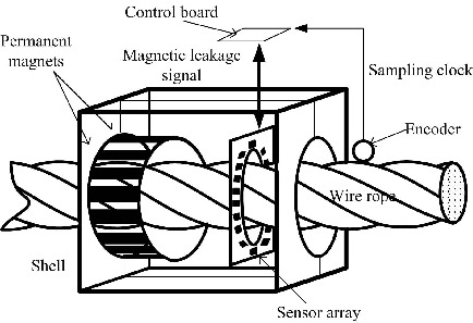
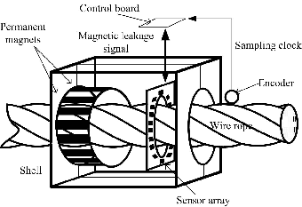
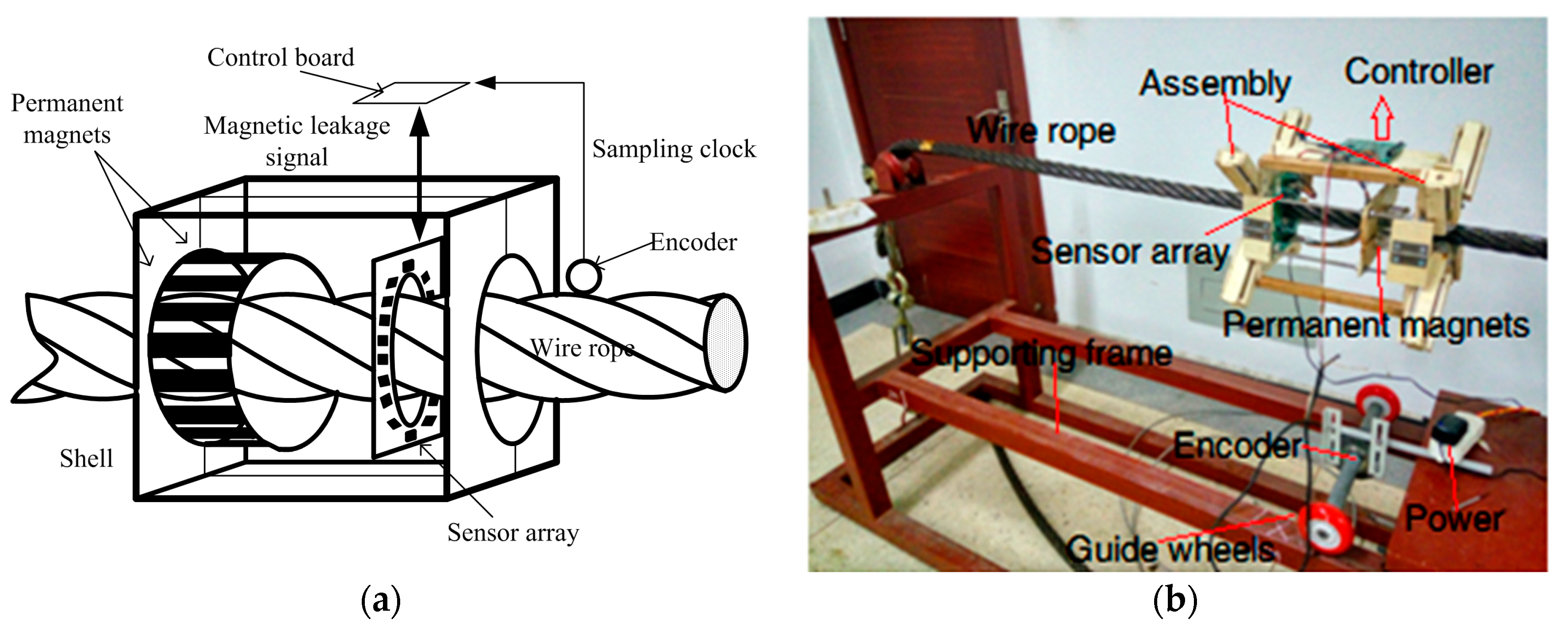
The principle of the proposed UME testing method is as shown in Figure 1. Permanent magnets were used as an excitation source, while ferromagnetic materials would be produced a weak magnetic field near external excitation. Considering this condition, the exciting rope would form a magnetic loop though the air, thus there is inner magnetic line in the rope. Once there was a defect in the excitation region, there was weak MFL signal caused by the defect. Considering a microscopic explanation, each electron rotating around the nucleus produces a loop circuit in normal conditions. According to Maxwell equations, loop circuits produce a stable magnetic field, but in stable ferromagnetic materials the magnetic fields offset each other because of untidy direction. However, under external magnetic field excitation, the magnetic fields produced by loop circuits would be uniform, then the rope would form a weak magnetic field. We can analyze the defect information by obtaining the weak magnetic field.
According to this principle, a prototype was manufactured to test wire rope local discontinuities in this paper. This device utilized 12 Nd–Fe–B permanent magnetic strips as the excitation source. The length of each strip was 28.6 mm, diameter was 4.7 mm, and remanence strength was 1.18 Tesla. Eighteen GMR sensors were uniformly distributed around the rope, with which an advanced RISC machine (ARM) was selected as the controller of the data-collection system. The number of sensors was confirmed according to the lift-off distance and sensors size. Sensors may be saturated because of small lift-off distance, and detection too close would scratch the wire rope while testing the rope. We hoped to employ many sensors to obtain circumferential high resolution of MFL distribution. However, when the detection distance is far, some small defects would not be tested well, even if it cannot be detected. After much experimental testing, when the diameter of sensor array board was 10 cm, sensors could sense the signal and most defects could be detected well. Thus, 18 GMR sensors were employed at most. To achieve the recognition of discontinuities, the following processing steps were applied in this paper, as shown in Figure 2.
2.1. Experimental Platform
The structure of the prototype is shown in Figure 3a, including system power module, analog signal modulation, encoder module, GMR sensor array, data storage control unit, and corresponding bypass.
The two analog signal modulations consisted of eight times preamplifier on GMR differential signal, then an additional circuit was used for impedance matching and lifting signal baseline. The voltage of the additive circuit was about 2 V after preamplifier. The system used equal-space sampling to acquire the weak MFL, and the pulse signal was produced by an encoder whose rotation perimeter was 0.31 m, sending 1024 pulses. With every pulse, the controller unit operated two analog-digital convertors(ADCs) on the 18 sensors’ output, then the 18-length array data was stored in an secure digital memory (SD) card. All the data was processed offline or transmitted to PC for further processing. System working frequency was 120 MHz, 18 GMR sensors were installed with switch devices, then transferred signal to ADC. The prototype object is shown in Figure 3b; the diameter of the detection array was 30 mm, the excitation source was about 15 cm away from the detection board, and magnetization spacing was 1.5 cm [22].
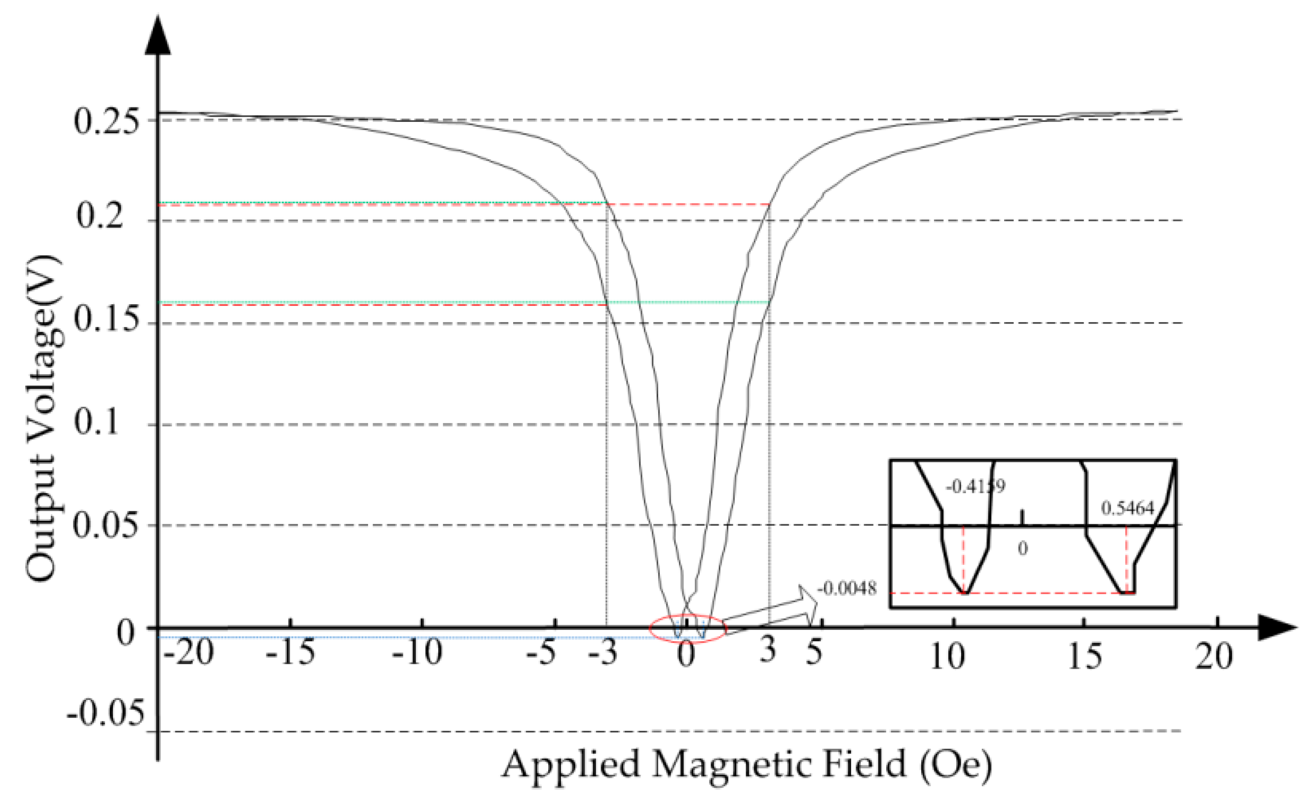
It is necessary to point out that the used GMR sensors had linear output when magnetic field varied between 0.5 and 3.0 Oe, and sensor sensitivity varied between 11 and 18 mV/V-Oe (the magnetic field strength corresponds to 11 and 18 mV multiplied by supply voltage). This sensor’s output is unipolar differential voltage; thus, the output is not affected by magnetic direction. Besides, because of the hysteresis effect, the sensor output would hysteretically export minimum voltage when the magnetic field direction changed from zero Oe. Thus, this sensor could export normal curve voltage to small defects, but big defects exported folding voltage curve. It can be a good feature to distinguish small and big defects. The GMR output curve when the temperature was 26 °C and supply voltage was 5 V is showed in Figure 4.
The traditional detection system in [9,10] needed to magnetize wire rope first, and the step may be repeatedly implemented until it is magnetized to form stable remanence. However, the remanence of wire rope would drop away after one week, and the rope need be magnetized again. The repetitive step increases maintenance time and cost contrasting with the UME detection method. More technology comparison details are showed in Table 1. It can be seen that the UME testing system has smaller size, lighter weight and simpler operation.
2.2. Data Preprocessing
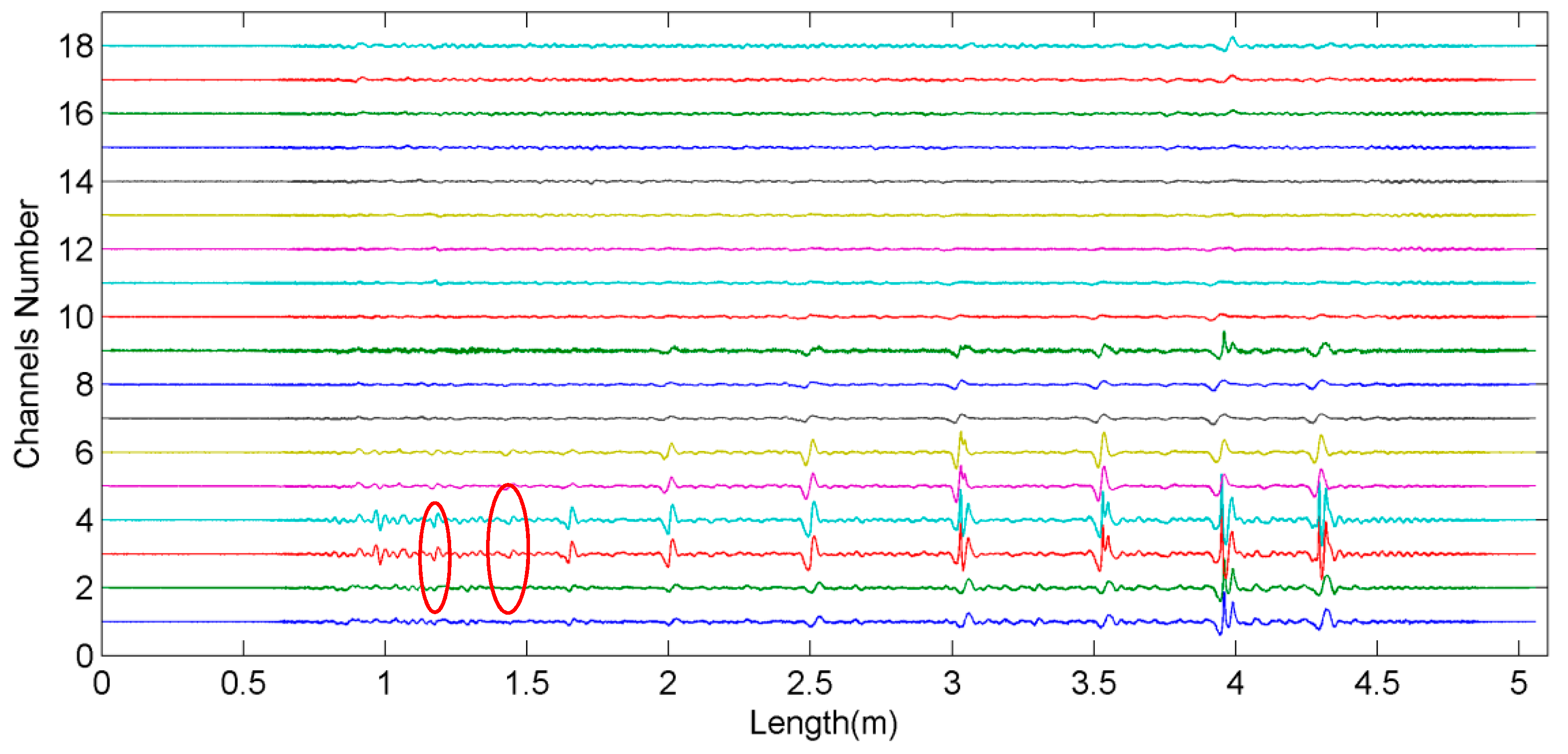
In the experiment, because the detection system could test wire rope of different diameters, we selected 28 mm and 30 mm diameter wire rope as testing specimens; their structure was 6 × 37(the rope consisted of 6 strands and each strand had 37 steel wires). Artificial defect types included one discontinuity to five and seven broken wires; moreover, each defect was destroyed as small gap, curling wires, and wide fracture. Besides, we tested the system performance of abrasive wire, and part defects of a specimen rope are shown in Figure 5. The length of this rope was 6 m, and its permitting detection was 4.5 m because of the magnetic pole. There was an abrasive defect at 1.1 m; 1.46 m and 1.67 m separately had a one-wire broken defect. There were two-wire broken defects at 1.22 and 2.02 m, three-wire broken defects at 2.52 m, five-wire broken defects at 3.04 and 3.54 m, seven-wire broken defects at 3.97 m, and four-wire broken defects at 4.31 m. The width of all small gaps was not more than 3 mm, the height of curling wires was about 0.5 cm, and wide fracture was about 1 cm.
Implementing the system to detect the specimen rope above, we acquired surface UME array signals, spreading the raw data by channel number, as shown in Figure 6. In the red circles, these singular signals were MFL signals of one or two broken wires in the gap condition.
It can be seen in Figure 6 that both ends had magnetic pole for magnetization. There the magnetic field strength exceeded sensor sensitivity range, thus there was no fluctuant curve. Besides, because of local magnetizing, sensor differences, and channel imbalance, the baseline of testing signal was not coherent. Thus, the data need to be preprocessed, including removing outliers and estimating baseline.
The magnetic field distribution is continuous in the air, therefore adjacent sampling points would not differ severely. We adopted Equation (1) to process the outliers, where the outlier was replaced by the mean of two adjacent points [23]:
where i is the channel number, j is the sampling length, and T is a threshold and was set as 50 in this paper.
After removing the outliers, a promoted subsection mean method was implemented to estimate the baseline of each signal, then removed to acquire the balanced MFL array signal. This method was based on the mean of MFL signal in a strand period of zero. The estimation algorithm was as shown in Equation (2):
where s(i) is the MFL signal without baseline, x(i) is the input signal, m is the sampling points of lay length, and N is the length of signal. According to the measurement, the lay length of specimen rope was about 3.1 cm, and combining the system sampling frequency we set the subsection as 102 points; that is to say, m is 52 in this paper. After estimating the baseline, the balanced array signal could be expanded as shown in Figure 7.
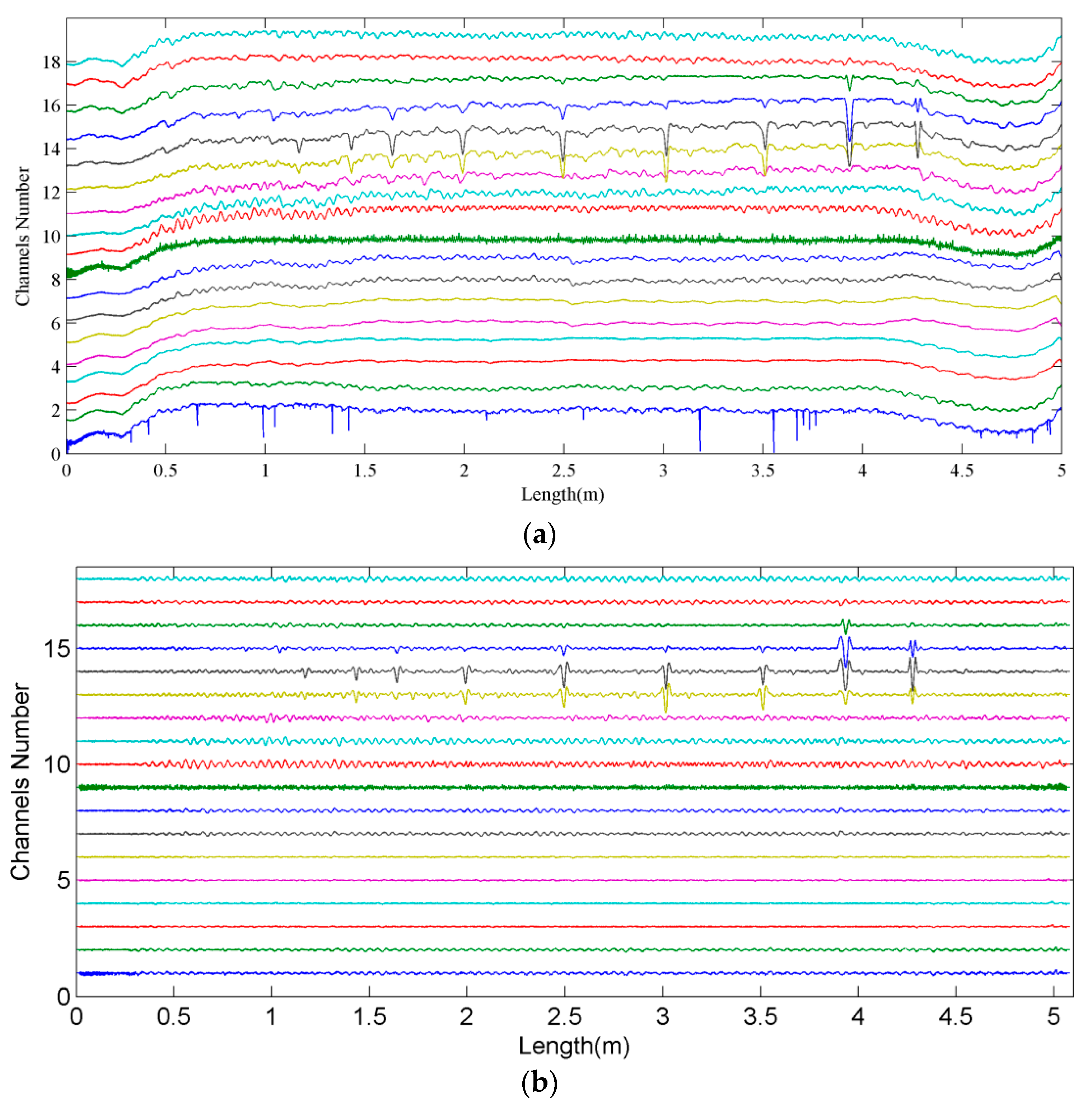
As a contrast, we tested the same wire rope by the remanence detection method. Figure 8a shows the raw remanence data of 18 channels; the remanence balance signal after implementing baseline estimation, the remanence balanced signals are shown in Figure 8b.
Contrasting Figure 7 with Figure 8b, both methods can detect the one-wire defects and the remanence signal amplitude is higher than UME at the detection sensor channel, but there is more noise in other channels. As for the UME signal, more channels can capture the weak MFL distribution, and there is less strand noise at all sensor channels. The remanence signal of a one-wire defect cannot be separated from the array signals because of strong strand noise. On the other hand, this signal processing algorithm has less computation than the [9,10], because this algorithm is a part of the previous work.
3. Image Processing
The preprocessing signal could be expanded as an asymmetrical sampling MFL image, and high-frequency axial sampling had abundant information, including helpful information to calculate circumferential MFL distribution. Thus, we proposed a down-sampling method to acquire multiframe symmetric sampling MFL images, then, using the SR method, reconstructed a high-resolution defect image. Before resolution enhancement, data must be transformed, filtered, located, and have defects extracted out, then the central image is normalized by translating the defect image [10]. Finally, the SR reconstruction method based on Tikhonov regularization was used to enhance image resolution. To achieve quantitative recognition discontinuities, we extracted a characteristic vector by selecting sensitive defect image descriptions.
3.1. Defect Image
3.1.1. Transformation and Filtering
A balanced MFL array signal was acquired after preprocessing. This data could be transferred to a two-dimensional gray image, with a mapping function as follows:
where L is the maximum gray value after transformation, f(x, y) is the array input, N is the minimum quantification value of ADC, Vs is the maximum sampling voltage, Vp is the maximum peak-to-peak voltage of amplifier, and f(i, j) is the output gray image.
Limiting sensor size, system axial frequency is much more than circumferential. In real sampling conditions, the voltage of axial neighboring domain does not vary obviously; the most variety was from quantization errors. Besides, the device would lightly swing then acquire circumferential MFL information in neighboring detection. Thus, the dense axial sampling contained much circumferential MFL information, and we could use this high-frequency sampling to forecast circumferential distribution through equal two-dimensional sampling. In this paper, axial sampling frequency was about nine times as much as that of circumferential sampling, thus the axial was down-sampled nine times to fit the circumferential sampling. We can obtain nine frames of MFL images of wire rope. We adopted Equation (4) to prove that the down sampling interval does not cause signal distortion.
According to signal decimation, a discrete signal x(n), assuming a down-sampling signal of y(n) = x(Mn), if their frequencies are in accord with fs ≥ 2Mfc, where fs is discrete sampling frequency and M is down-sampling interval, the DTFT of signal y(n) and x(n) is satisfied as follows:
According to Equation (4), the spectrum of down-sampling signal was extended M times, then shifted 2πk/M (k = 1, 2, ..., M–1) and superposed together; moreover, the amplitude was reduced nine times but y(n) was equivalent to x(n). Figure 9a shows a balanced signal block from the testing results above, and Figure 9b shows the spectrums of balanced and down-sampling signals, where frequency of peak value conformed to a nine-time relationship and there was no frequency aliasing. Thus, the nine-times down-sampling signal was equivalent to raw signal and there was no signal distortion.
These new images combined noise, such as pulse noise, strand waves, and converted noise. A mean filter mask was applied to restrain the noise. Then, utilizing a second-order derivative mask to sharpen images, we get:
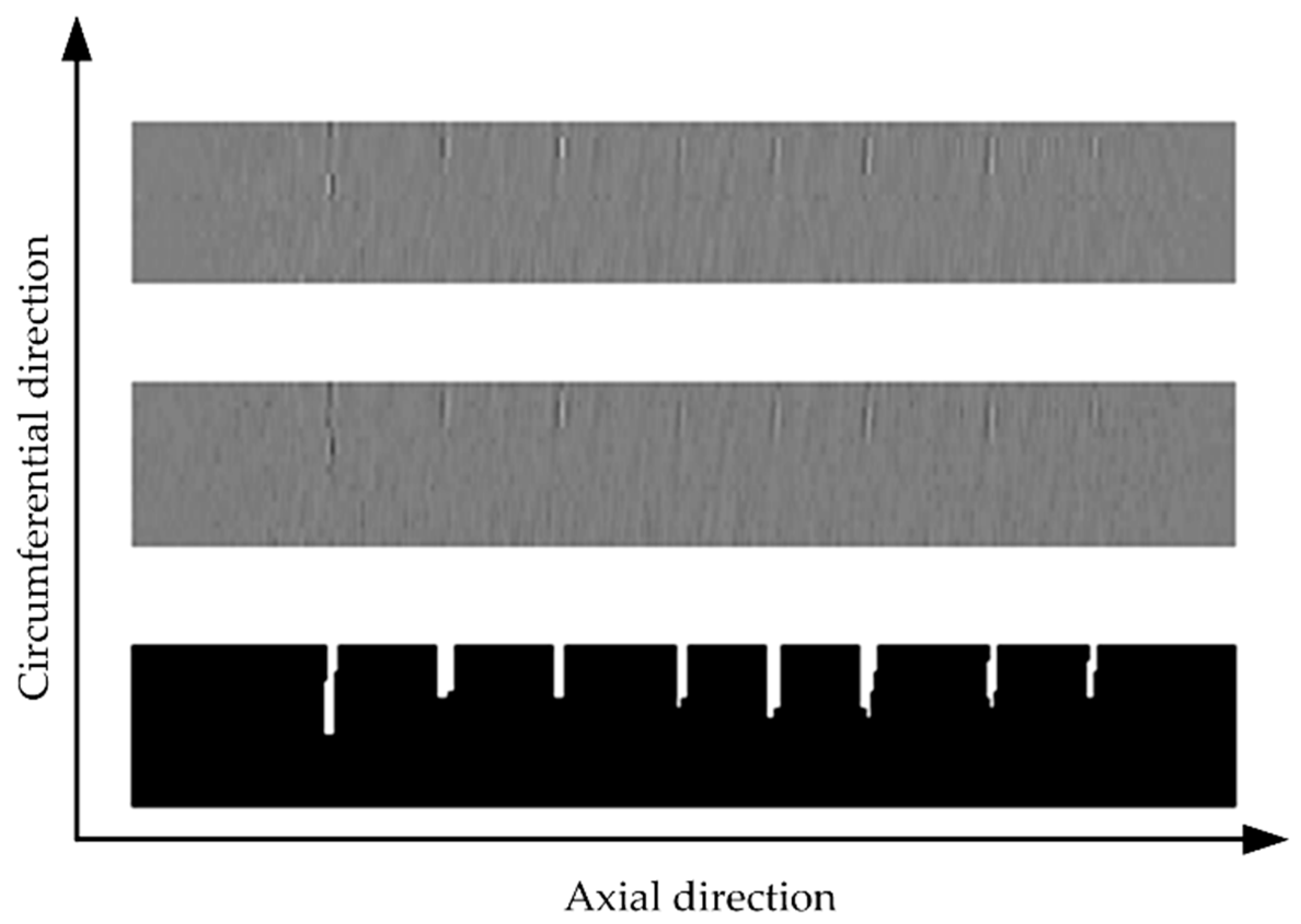
The down-sampling image is shown in the top section of Figure 10, and the middle one was filtered and sharpened. Canny edge detector was applied to get the locations of defects, and to avoid the influence of weak region, we performed an expand and corrosion operation where structure elements were separately a 3 × 3 mask and 3 × 1 mask. Defect regions after this process are shown in the bottom section of Figure 10. The contrast of all pictures was enhanced for defect visualization.
3.1.2. Segmentation and Normalization
After locating defects, defect regions need to be segmented along the axis of the rope. In this paper, the projection method was utilized to obtain positional information of two dimensions. First, the binary image was projected to transverse with the sum and let the curve binary, then the derivative of this curve was calculated, with the axial starting position of the defect shown with 1 and the end shown with −1. To acquire accurate positions of defects, we calculated the maximum and minimum in the target region, the center of the two values was considered the new central point, and we again extracted defect images 18 points long. After processing all down-sampling gray images, each defect UME defect had a nine-frame picture.
To guarantee that all the centers had similar position, the center of the image needed to be normalized. On the basis of the first frame image, its central coordinate was (9, jc); when jc was less than 9, the image needed to be processed as follows:
when jc was more than 9, the image needed to be processed as follows:
and when jc was 9, there was no transformation, where f(i, j) is the image before being transformed and g(i, j) is the normalized image. Taking the wire rope from Section 2.2 as an example, the primary resolution MFL image and down-sampling images are shown in Figure 11, and the contrast of all images was increased for defect visualization.
3.2. Image Super-Resolution Reconstruction
Super-resolution is an image restoration technique that utilizes low-resolution images to rebuild a high-resolution image. We acquired nine-frame UME pictures of each defect, so that a multiframe image reconstruction technique could be used to rebuilt high-resolution images. For an image degeneration process, the mathematical model can be described as follows:
where X, Y, and E are high-resolution image, low-resolution image, and noise, respectively. B is a fuzzy convolution matrix and D is a down-sampling matrix, and we can replace W = DB. It is an ill-posed problem that X was reconstructed by Y because of multisolution or non-solution. To solve this problem, a classical method named Tikhonov regularization, which is based on remaining raw data to solve a solution by satisfying a priori constraints, was used [24]. The regularization process could be divided into two methods, deterministic regularization and random regularization. In this paper, first the regularization method was performed to optimize the problem in order to make it solvable. This was done through a minimization cost function [24]:
where ‖Y − WX‖2 is the error term, λ is the regularization parameter used to balance the relationship between error and high-frequency energy, ‖CX‖2 is the penalty term, and C is a high-pass filter. In general, natural images have finite smooth continuity, and this condition is a constraint term for the convex Function (9) and recovering X by an iteration procession as follows:
where α is the step size, ck is the weight coefficient of each frame image, λk is the regularization parameter, and P is the number of frames per image.
Multiframe image super-resolution reconstruction based on the Tikhonov regularization step was as follows:
- Step one: Calculate mapping parameter between images.
- First, initialize affine shifting set.
- For i = 2:P.
- Register current image to first frame: compute the Lucas–Kanade optical using a Gaussian pyramid for the two images in each level.
- End.
- Step two: Divide image mesh, simulate the basic image as a high-resolution image with spine interpolation.
- Step three: Regularize adaptive super-resolution based on Tikhonov:
- Initialize output
- while iter < 200 or Variation < 10−4
- calculate , , and ;
- For k = 1:P–1
- Perform (10)
- End
- Calculate Variation as ;
- iter++;
- End.
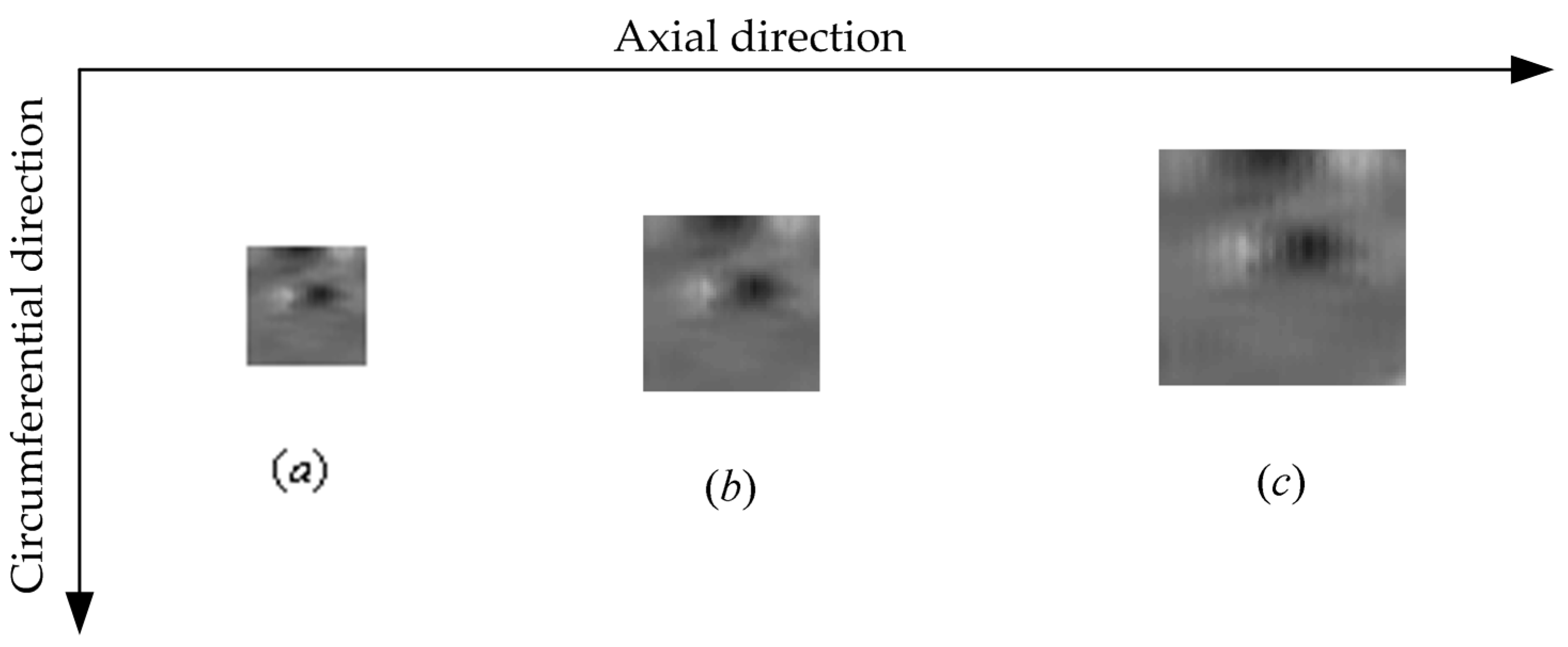
To reduce computation, we did not use the step, weight, and regularization parameter selection principle of [24], but the step was set as 0.2, the weight coefficient was 1, and the regulation parameter was 0.01. Double, triple, and quadruple resolution reconstruction images are shown in Figure 12. Also, the contrast of the three images was enhanced for defect visualization.
Contrasting the three reconstruction results, excessive resolution reconstruction would produce jagged contour when other parameters and input images were the same. However, the image contrast of low-resolution SR results was higher than the high-resolution reconstruction. Contrasting the three pictures of Figure 12, when SR result was triple the computation and image property was the best, its resolution was 53 × 53. Thus, we set the resolution reconstruction number as three in this paper.
3.3. Defect Description
To achieve quantitative recognition, direct image input will increase the computation, so it is necessary to extract a description of the image. In addition, image characteristics must be sensitive when reducing image dimensionality. We selected parts of sensitive features from [10], where the statistical texture features and seven invariant moments were described as defect image.
Image texture features are based on image pixel grayscale statistics, which usually include average brightness, average contrast, relative smoothness, third-order moment, conformance, and entropy. We implemented an experimental screening, which was achieved by variable control. Finally, experimental recognition results showed that average contrast, third-order moment, conformance, and entropy were more sensitive than other texture features. The basis of this statistical texture is the image’s histogram, and describing the shape distribution of the histogram relies on the central moment, which is defined as
where n is the order of the moments, p(zi) is the normalized histogram, L is a random quantity of gray level zi, and m is the average brightness:
The average contrast is defined as
which is the standard deviation of the image. It reflects the average change in the image. The third-order moment is defined as
If the histogram is symmetric, u3 is zero; if the skewness tends to the right, the value is positive; but if it tends to the left, the value is negative. The conformance is defined as
where, when the image is constant, U is maximum. The entropy reflects the degree of randomness in the gray-level values, and is defined as
The invariant moment characteristic is based on a statistical analysis of the gray distribution of an image. It describes all the features of the object from an overall view, which is not easily affected by noise, shifting, rotation, or changes in the size of the image. After experimental selection, odd order invariant moments were more sensitive than other moments by variable control. Thus, we just selected the odd order features of seven order invariant moments.
For an image f(x, y), varied order exists if it is continuous in block, and there is a limited non-zero number available in the image. The (p + q)th order moment of f(x, y) is defined as
The central moments are defined as
where x’ = m10/m00, y’ = m01/m00; that is to say, they are the gravity of the image. By calculating the different central moments, the odd order invariant moments are defined as
Characteristic description is the bridge of classification and image. In this paper, part defect images were processed by all the algorithms above, and the selected sensitive description vectors are shown in Table 2. The invariant moments were processed by absolute value of logarithm to reduce the range of variation, because the value of invariant moments is very small, except the invariance and modulus of moments are important.
4. Classification
RBF neural network [10,13] is better than BP in convergence rate learning and local approximation performance, because minority weights will locally influence net output in local input sets. Thus, RBF was successful in applying an approximation of nonlinear function, time series analysis, data analysis, pattern recognition, information processing, image processing, system modeling, controlling, and fault diagnosis.
The basic idea of RBF is that solved problems are linearized by mapping nonlinear input to high-dimensional space, where the Gaussian function is usually chosen as a transformation function. A simple RBF neural network has a three-layer mapping structure, which includes an input, a hidden layer, and an output layer. The input layer consists of sensing units, which are used to link the outer data and the inner network. The hidden layer is a high-dimensional mapping structure of kernel function, which transforms the nonlinear data to a linearly divisible set. Moreover, the linear output layer fits a curve in the high-dimensional dataset that is optimally equal, to find divisional surfaces in the hidden layer set. Once the central position of the activated distance function is confirmed in the hidden layer, the relationship of input and output is also confirmed, and the output is the linear sum of hidden units. The RBF neural network usually utilizes a distance function (such as Euclidean distance) as the basic function of hidden nodes and adopts a radial basis function (such as Gaussian function) as the activation function. The radial basis function is a radial symmetric about the central point of an n-dimensional space. Once the input of a neural unit is far away from the central point, the activation degree of this unit is low. This feature is generally named as a local characteristic of the hidden layer.
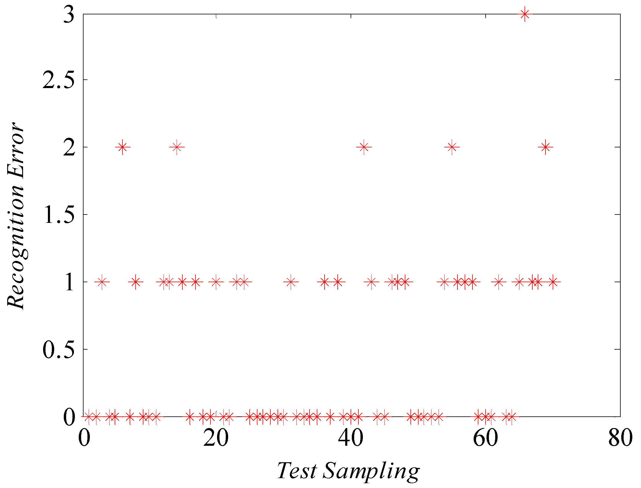
There were 281 artificial defects of broken wires, curling wires, and wide fractures by using the UME. To enhance reliability and generalization, the neural network was trained by a set of 211 randomly selected samples, and the others were used to test the network recognition accuracy. We adopted the MATLAB (2013a, Mathworks Inc. Natick, MA, USA, 2013) neural network toolbox to design an RBF neural network, where “newnpp” could quickly establish a classification network. The designed network consisted of three layers, an input with a number of input vectors and the distance function as the activation function. The hidden layer was a competitive layer without threshold values, and the input of this layer was the distance between the input vectors and sample vectors. The probability of each element was calculated by the competitive transfer function. The output of the function was 1, while the maximum probability of the other elements was 0. The radial spread parameter was 0.145, and the hidden nodes adopted the automatic optimization strategy. The activation function of the hidden layer was the “compet” function, and the output was a vector of seven elements, where the number of broken wires was only the target element with an output of 1. The network training accuracy was 95.26% and the average training error was 0.0616. The maximum recognition error was three broken wires in the network testing, and with one limited error the recognition accuracy was 91.43%. The testing performance of different parametersis shown in Table 3. The recognition accuracy is low in Table 3. Different diameters of wire rope may cause this result. On the other hand, lift-off distance, magnetization and shaking of detection equipment also would cause singular signal. Slow detection, modified magnetization and more characteristics may have a good influence on the recognition accuracy.
5. Conclusions
A novel UME wire rope detection method was proposed in this paper. According to the MFL production principle, a prototype was manufactured with small volume, light weight, and convenient installation. We detected enough broken wire defects in the experiment, and the baseline signal was estimated by the subsection mean method. Then digital image processing was adopted to filter the quantification noise. To improve the image circumferential resolution, an MFL image SR method was proposed with Tikhonov regular. Finally, the most sensitive characteristics were selected through the variable control method, and an RBF neural network was designed to quantitatively classify broken wires. The experimental work can be summarized as follows:
- The proposed detection method could effectively test various types of defects of wire rope, even abrasion and small gaps.
- Based on Tikhonov regular SR reconstruction methods, image features of defects could effectively remain while the axial resolution was reduced and circumferential resolution was increased.
- The proposed detection system, signal processing, and image processing method were applicable and general to other testing conditions. The accuracy of the RBF neural network was high, and it was easy to achieve online testing with the system algorithm. The testing results could provide reliable information for estimation of the lifespan of wire rope.
Author Contributions
X.T. designed and performed the experiments, then analyzed the data and wrote the paper; J.Z. provided the experimental platform, supported funding, and corrected the paper.
Acknowledgments
This work is partially supported by the National Natural Science Foundation of China (Grant No. 61040010, 61304144), Key Technologies R&D Program of Henan Province (Grant No. 152102210284), the science and technology program of the Henan Education Department (Grant No.17A510009), and the Technology Development Cooperation Project of Henan Province (182106000026).
Conflicts of Interest
The authors declare no conflicts of interest.
References
- Li, J.Y.; Tian, J.; Zhou, J.; Wang, H.; Meng, G.; Liu, T.Y.; Deng, T.; Tian, M. Literature Review of Research on the Technology of Wire Rope Nondestructive Inspection in China and Abroad. MATEC Web Conf. 2015, 22, 03025. [Google Scholar] [CrossRef]
- Amineh, R.K.; Nikolova, N.K.; Reilly, J.P.; Hare, J.R. Characterization of Surface-Breaking Cracks Using One Tangential Component of Magnetic Leakage Field Measurements. IEEE Trans. Magn. 2008, 44, 516–524. [Google Scholar] [CrossRef]
- Liu, B.; He, L.-Y.; Zhang, H.; Cao, Y.; Fernandes, H. The axial crack testing model for long distance oil-gas pipeline based on magnetic flux leakage internal inspection method. Measurement 2017, 103, 275–282. [Google Scholar] [CrossRef]
- Feng, J.; Lu, S.; Liu, J.; Li, F. A Sensor Liftoff Modification Method of Magnetic Flux Leakage Signal for Defect Profile Estimation. IEEE Trans. Magn. 2017, 53, 6201813. [Google Scholar] [CrossRef]
- Zhang, D.L.; Zhao, M.; Zhou, Z.H. Quantitative Inspection of Wire Rope Discontinuities using Magnetic Flux Leakage Imaging. Mat. Eval. 2012, 70, 872–878. [Google Scholar]
- Wang, H.-Y.; Xu, Z.; Hua, G.; Tian, J.; Zhou, B.-B.; Lu, Y.-H.; Chen, F.-J. Key technique of a detection sensor for coal mine wire ropes. Min. Sci. Technol. 2009, 19, 170–175. [Google Scholar] [CrossRef]
- Basak, D.; Pal, S.; Basak, P.; Palit, D.; Patranabis, D.C. A connectionist model for lock coil rope fault prediction. Insight 2008, 50, 501–505. [Google Scholar] [CrossRef]
- Sharatchandra Singh, W.; Rao, B.P.C.; Mukhopadhyay, C.K.; Jayakumar, T. GMR-based magnetic flux leakage technique for condition monitoring of steel track rope. Insight Non-Destr. Test. Cond. Monit. 2011, 53, 377–381. [Google Scholar] [CrossRef]
- Zhang, J.; Tan, X. Quantitative Inspection of Remanence of Broken Wire Rope Based on Compressed Sensing. Sensors 2016, 16, 1366. [Google Scholar] [CrossRef] [PubMed]
- Zhang, J.W.; Tan, X.J.; Zheng, P.B. Non-Destructive Detection of Wire Rope Discontinuities from Residual Magnetic Field Images Using the Hilbert-Huang Transform and Compressed Sensing. Sensors 2017, 17, 19. [Google Scholar] [CrossRef] [PubMed]
- Cao, Y. Study on Wire Rope Local Flaw Quatitative Testing based on MFL Imaging Principle. Ph.D. Dissertation, Harbin Institute of Technology, Harbin, China, 2007; pp. 22–27. (In Chinese). [Google Scholar]
- Zhang, D.; Zhao, M.; Zhou, Z.; Pan, S. Characterization of wire rope defects with gray level co-occurrence matrix of magnetic flux leakage images. J. Nondestruct. Eval. 2013, 32, 37–43. [Google Scholar] [CrossRef]
- Cao, Q.; Liu, D.; He, Y.; Zhou, J.; Codrington, J. Nondestructive and quantitative evaluation of wire rope based on radial basis function neural network using eddy current inspection. NDT & E Int. 2012, 46, 7–13. [Google Scholar] [CrossRef]
- Goktepe, M. Non-destructive crackdetection by capturing local flux leakage field. Sens. Actuators A Phys. 2001, 90, 70–72. [Google Scholar] [CrossRef]
- Xu, F.; Wang, X.; Wu, H. Inspection method of cable-stayed bridge using magnetic flux leakage detection: Principle, sensor design, and signal processing. J. Mech. Sci. Technol. 2012, 26, 661–669. [Google Scholar] [CrossRef]
- Park, S.; Kim, J.-W.; Lee, C.; Lee, J.-J. Magnetic Flux Leakage Sensing-Based Steel Cable NDE Technique. Shock Vib. 2014, 2014, 1–8. [Google Scholar] [CrossRef]
- Raisutis, R.; Kazys, R.; Mazeika, L.; Samaitis, V.; Zukauskas, E. Propagation of Ultrasonic Guided Waves in Composite Multi-Wire Ropes. Materials 2016, 9, 451. [Google Scholar] [CrossRef] [PubMed]
- Peng, P.-C.; Wang, C.-Y. Use of gamma rays in the inspection of steel wire ropes in suspension bridges. NDT & E Int. 2015, 75, 80–86. [Google Scholar] [CrossRef]
- Zhang, D.; Zhou, Z.; Sun, J.; Zhang, E.; Yang, Y.; Zhao, M. A Magnetostrictive Guided-Wave Nondestructive Testing Method With Multifrequency Excitation Pulse Signal. IEEE Trans. Instrum. Meas. 2014, 63, 3058–3065. [Google Scholar] [CrossRef]
- Cottis, R.A.; Homborg, A.M.; Mol, J.M.C. The relationship between spectral and wavelet techniques for noise analysis. Electrochim. Acta 2016, 202, 277–287. [Google Scholar] [CrossRef]
- Kwaśniewski, J. Application of the Wavelet Analysis to Inspection of Compact Ropes Using a High-Efficiency Device/Analiza falkowa efektywnym narzędziem diagnostyki lin kompaktowanych. Arch. Min. Sci. 2013, 58. [Google Scholar] [CrossRef]
- Zhang, J.; Tan, X.; Chen, Y. An Open Micro Magnetic Excitation Wire Rope Damage Detection System. Patent No. CN206772899U, 3 May 2017. [Google Scholar]
- Mukherjee, D.; Saha, S.; Mukhopadhyay, S. An adaptive channel equalization algorithm for MFL signal. NDT & E Int. 2012, 45, 111–119. [Google Scholar] [CrossRef]
- He, H.; Kondi, L.P. An Image Super-Resolution Algorithm for Different Error Levels Per Frame. IEEE Trans. Image Process. 2006, 3, 592–603. [Google Scholar] [CrossRef]
Figure 1.
The principle of the unsaturated magnetic excitation (UME) testing method. The solid line represents the magnetic loop of the excitation source; the dotted line represents the wire rope inner magnetic field.
Figure 1.
The principle of the unsaturated magnetic excitation (UME) testing method. The solid line represents the magnetic loop of the excitation source; the dotted line represents the wire rope inner magnetic field.

Figure 2.
Discontinuity recognition flow chart.
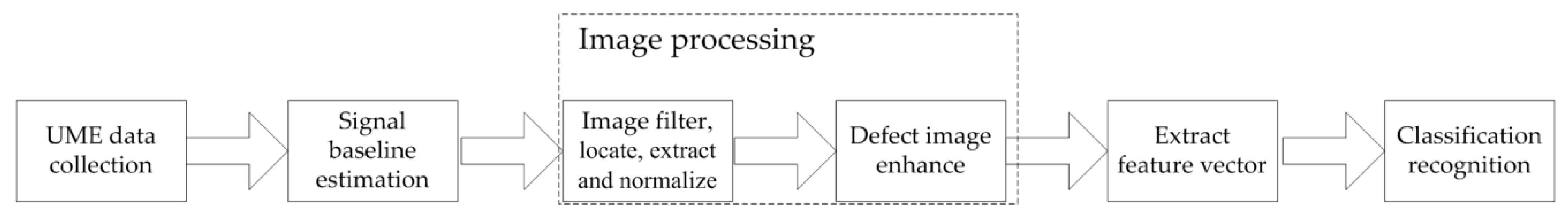
Figure 3.
(a) The structure of the prototype; (b) the object of experimental application.

Figure 4.
Giant magneto resistance (GMR) sensor output under 25 °C.

Figure 5.
Manufacturing standard small gap defects: (a) worn wire at 1.1 m; (b) two wires broken at 1.22 m; (c) one wire broken at 1.46 m; (d) one wire broken at 1.67 m; (e) two wires broken at 2.02 m; (f) three wires broken at 2.52 m; (g) five wires broken at 3.04 m; (h) five wires broken 3.54 m; (i) seven wires broken at 3.97 m; (j) four wires broken at 4.31.
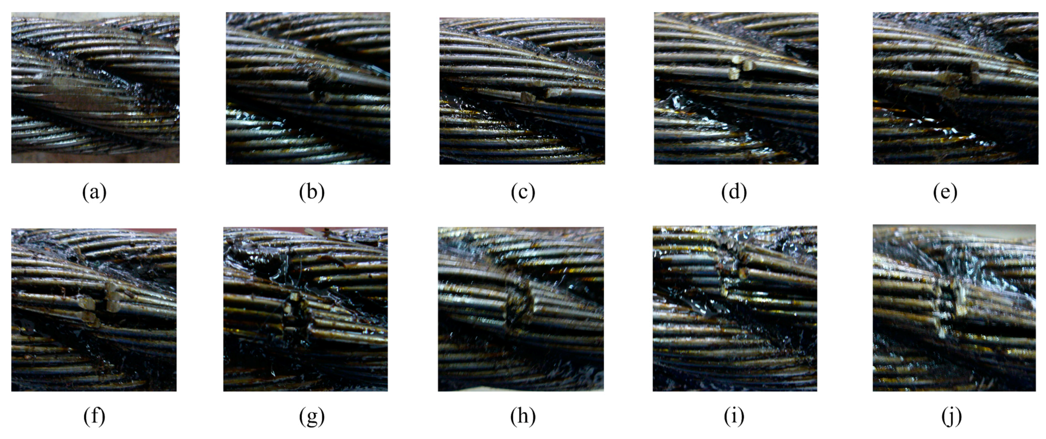
Figure 6.
UME raw testing of magnetic flux leakage (MFL) signals of 18 channels.
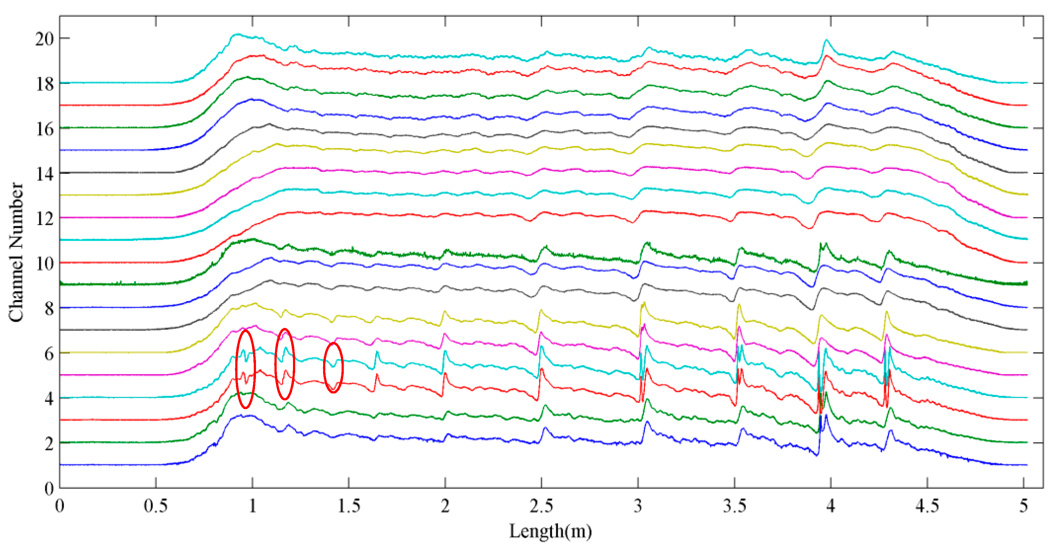
Figure 7.
Expanded UME estimated signal by channel number, circles show one broken gap condition signal was circled at 1.22 and 1.46 m.
Figure 7.
Expanded UME estimated signal by channel number, circles show one broken gap condition signal was circled at 1.22 and 1.46 m.

Figure 8.
(a) Raw remanence signal of 18 channels; (b) balanced remanence signal after baseline estimation.
Figure 8.
(a) Raw remanence signal of 18 channels; (b) balanced remanence signal after baseline estimation.

Figure 9.
(a) A defect balanced signal block of one channel; (b) spectrums of primary sampling and down-sampling.
Figure 9.
(a) A defect balanced signal block of one channel; (b) spectrums of primary sampling and down-sampling.
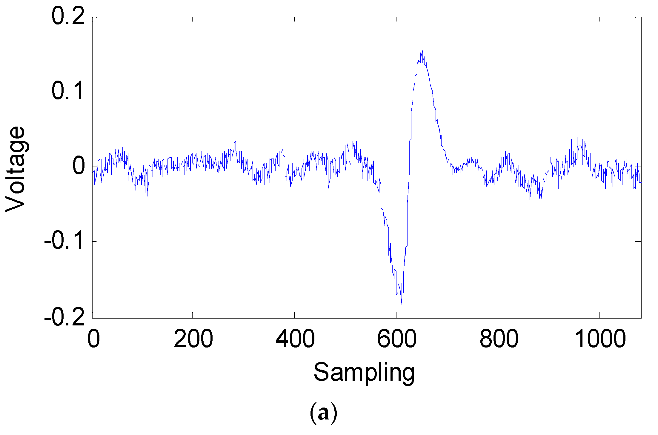
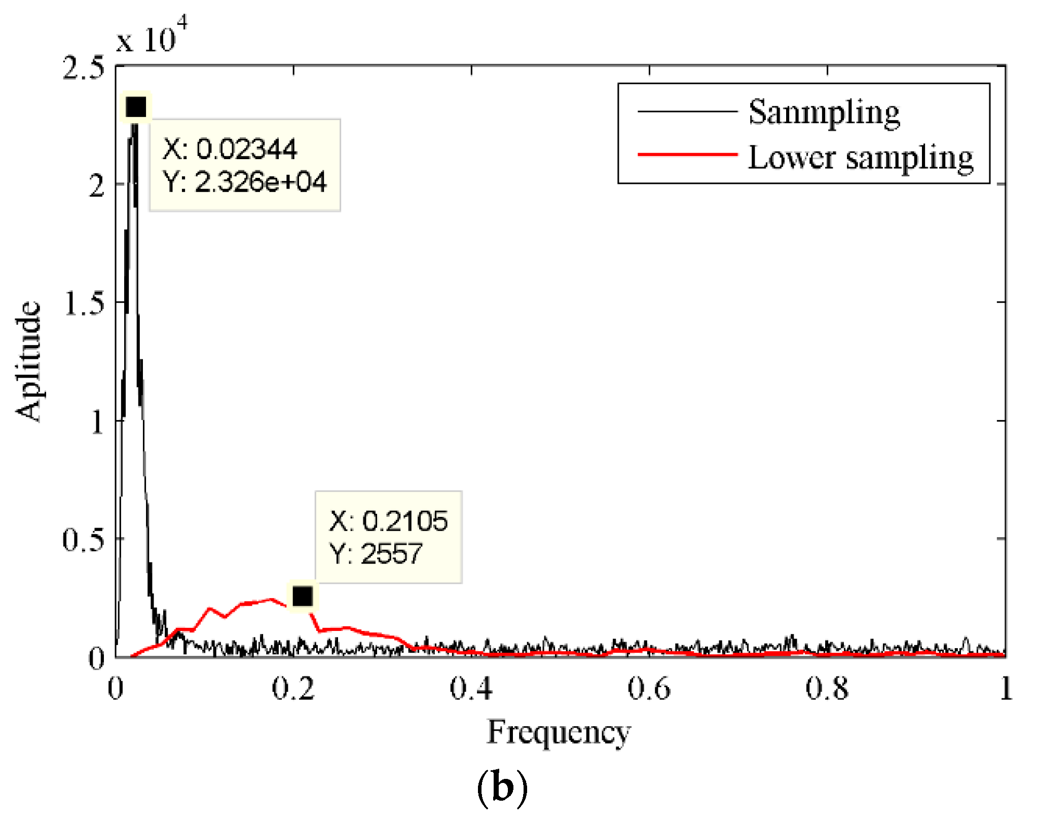
Figure 10.
Raw down-sampling gray image (top); sharpened defect image (middle); and defect location image (bottom). In the first location were two defects along the circumference with one and two broken wires.
Figure 10.
Raw down-sampling gray image (top); sharpened defect image (middle); and defect location image (bottom). In the first location were two defects along the circumference with one and two broken wires.

Figure 11.
Primary resolution image and low-resolution images: (a) primary resolution; (b–j) down-sampling images.
Figure 11.
Primary resolution image and low-resolution images: (a) primary resolution; (b–j) down-sampling images.
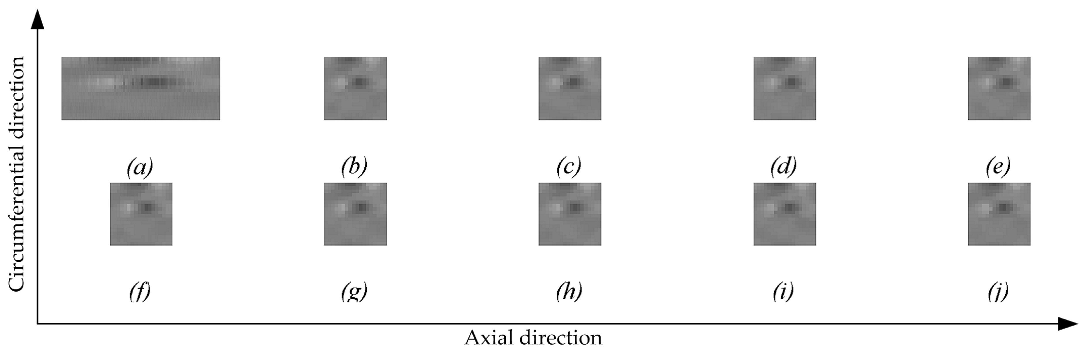
Figure 12.
Different resolution reconstruction results: (a) double resolution reconstruction image; (b) triple resolution reconstruction image; (c) quadruple resolution reconstruction image.
Figure 12.
Different resolution reconstruction results: (a) double resolution reconstruction image; (b) triple resolution reconstruction image; (c) quadruple resolution reconstruction image.

Figure 13.
Recognition distribution of error when “spread” was 0.145.


Table 1.
Comparison of the remanence device with UME.
| Method | Testing Step | Value (dm2) | Weight (kg) | Detection Time (s) |
|---|---|---|---|---|
| Remanence | Detection after magnetizing | 11.5 | 2.5 | 30+ 1,2 |
| UME | Direct detection | 6.5 3 | 1 3 | 24 1 |
1 Detection speed of remanence was the same as UME, and slow testing speed can guarantee compete sampling; 2 Magnetizing time of remanence was 6 s every time, and it mostly needed to be implemented more than three times in the experiment; 3 Core components were transplanted to a remanence assembly.
Table 2.
Part defect sensitive characteristic vectors.
| Broken Wires | σ | u3 × 10−4 | U × 10−2 | e | M1 | M3 | M5 | M7 |
|---|---|---|---|---|---|---|---|---|
| 1 | 5.33 | −7.11 | 6.1446 | 4.3744 | 6.6409 | 30.9157 | 57.4199 | 58.6916 |
| 2 | 9.08 | 77.47 | 5.0684 | 4.8489 | 6.6487 | 29.2743 | 55.5046 | 59.2687 |
| 3 | 11.03 | 18.17 | 6.3782 | 4.7540 | 6.6390 | 30.5603 | 55.9229 | 57.8301 |
| 4 | 15.07 | 158.12 | 3.7091 | 5.4579 | 6.6519 | 28.0789 | 55.1216 | 53.8476 |
| 5 | 22.18 | 596.7 | 2.8029 | 5.9044 | 6.6520 | 28.0685 | 52.8666 | 52.6630 |
| 7 | 20.71 | 170.74 | 4.1813 | 5.6123 | 6.6389 | 27.8631 | 54.5276 | 52.9025 |
Table 3.
Performance of the designed RBF neural network.
| Spread | Maximum Error | Average Error | Training Accuracy | Recognition Accuracy | One Error Accuracy |
|---|---|---|---|---|---|
| 0.11 | 4 | 0.6714 | 99.53% | 52.86% | 87.14% |
| 0.145 | 3 | 0.5429 | 95.26% | 55.71% | 91.43% |
| 0.18 | 3 | 0.5143 | 91.00% | 58.57% | 91.43% |
| 0.215 | 3 | 0.5 | 86.73% | 60% | 91.43% |
© 2018 by the authors. Licensee MDPI, Basel, Switzerland. This article is an open access article distributed under the terms and conditions of the Creative Commons Attribution (CC BY) license (http://creativecommons.org/licenses/by/4.0/).
Share and Cite
MDPI and ACS Style
Tan, X.; Zhang, J. Evaluation of Composite Wire Ropes Using Unsaturated Magnetic Excitation and Reconstruction Image with Super-Resolution. Appl. Sci. 2018, 8, 767. https://doi.org/10.3390/app8050767
AMA Style
Tan X, Zhang J. Evaluation of Composite Wire Ropes Using Unsaturated Magnetic Excitation and Reconstruction Image with Super-Resolution. Applied Sciences. 2018; 8(5):767. https://doi.org/10.3390/app8050767
Chicago/Turabian StyleTan, Xiaojiang, and Juwei Zhang. 2018. "Evaluation of Composite Wire Ropes Using Unsaturated Magnetic Excitation and Reconstruction Image with Super-Resolution" Applied Sciences 8, no. 5: 767. https://doi.org/10.3390/app8050767
Note that from the first issue of 2016, this journal uses article numbers instead of page numbers. See further details here.