Rheological and Flocculation Analysis of Microfibrillated Cellulose Suspension Using Optical Coherence Tomography


1
VTT Technical Research Centre of Finland Ltd., P.O. Box 1603, FI-40101 Jyväskylä, Finland
2
Optoelectronics and Measurement Techniques Unit, Faculty of Information Technology and Electrical Engineering, University of Oulu, P.O. Box 4500, FI-90014 Oulu, Finland
3
Department of Physics, University of Jyvaskyla, P.O. Box 35, FI-40014 Jyväskylä, Finland
4
Spinnova Ltd., Palokärjentie 2-4, 40320 Jyväskylä, Finland
*
Author to whom correspondence should be addressed.
Appl. Sci. 2018, 8(5), 755; https://doi.org/10.3390/app8050755
Submission received: 23 February 2018
/
Revised: 1 May 2018
/
Accepted: 7 May 2018
/
Published: 10 May 2018
(This article belongs to the Special Issue Optical Coherence Tomography and its Applications)
Abstract
:Featured Application
Optical coherence tomography brings excellent new possibilities for improving and extending existing rheological measurement devices and methods.
Abstract
A sub-micron resolution optical coherence tomography device was used together with a pipe rheometer to analyze the rheology and flocculation dynamics of a 0.5% microfibrillated cellulose (MFC) suspension. The bulk behavior of the MFC suspension showed typical shear thinning (power-law) behavior. This was reflected in a monotonously decreasing floc size when the shear stress exceeded the yield stress of the suspension. The quantitative viscous behavior of the MFC suspension changed abruptly at the wall shear stress of 10 Pa, which was reflected in a simultaneous abrupt drop of the floc size. The flocs were strongly elongated with low shear stresses. With the highest shear stresses, the flocs were almost spherical, indicating a good level of fluidization of the suspension.
1. Introduction
Microfibrillated cellulose (MFC) is a material of high interest due to its sustainability and biodegradability, and unique properties such as, mechanical robustness, barrier properties, large surface area, and lightness [1,2]. Over the past decade, there has been explosive growth in MFC research, including improved MFC production technologies, surface functionalization, characterization techniques, composites processing, self-assembly, optical properties, and barrier properties. The applications of MFC are already numerous including supercapacitors, transparent flexible electronics, batteries, barrier/separation membranes, and antimicrobial films [3].
A frequently noted issue in the processing of MFC suspensions is their complex rheological behavior. MFC suspensions tend to form a strong gel, which shows, for example, yield stress, shear thinning, hysteresis, and thixotropy already in low mass concentrations. Rheological information is critical in the design and operation of, for example, pumping, mixing, storage, and extrusion processes. MFC is also commonly used as a rheology modifier, for example, in cements, inks, drilling fluids and cosmetics. Thus, the bulk rheology of MFC suspensions has been a popular subject of discussion [4,5,6].
Due to a high aspect ratio of fibres and strong interfibrillar forces, MFC fibres flocculate easily and form a highly entangled network already at relatively low concentrations. Thus, in addition to rheology, the flocculation tendency of MFC fibres has been of interest [7,8,9]. As summarized in [9], at the macroscale, that is, at the rheometer scale, changes in the floc structure of MFC correlate with a change in the shear stress. At low shear stress, flocs are attached to each other. When shear stress is increased, the floc structure starts to yield via flocs separating from each other. At high shear stresses, fibrils flow in individual, detached flocs, the size of which is inversely proportional to the shear stress.
Previously the flocculation of MFC has been studied in a transparent cylindrical rheometer geometry [7,8,9]. Here, we analyze the flocculation of a MFC suspension in a pipe flow, which is a more realistic geometry for many practical applications. The flocculation measurements were performed when preparing our recently published article Ref. [10]. In that paper, we used a combination of pipe flow, pressure loss measurement, and a high-speed, sub-micron resolution Doppler optical coherence tomography (DOCT) device for investigating the rheology of 0.5% MFC suspension. DOCT was used in measuring the stationary velocity profiles of the MFC flow in the near-wall region of a straight tube. In addition to analysing the bulk rheology (yield stress and viscous behavior) using the concept of velocity profiling rheometry, the wall/depletion layer dynamics of the suspension was studied there in detail. The novel flocculation analysis presented in this paper is based on the structural information obtained simultaneously with the velocity information. The results in [10] that are relevant to this study are briefly presented.
2. Materials and Methods
The microfibrillated cellulose sample was prepared from never-dried bleached kraft birch pulp via grinding three times in a supermasscolloider (Masuko Sangyo Co. Ltd., Kawaguchi, Saitama-pref., Japan). Prior to grinding, the pulp was changed to its sodium form and washed with deionized water, to obtain an electrical conductivity less than 10 µS/cm, according to a procedure introduced by [11]. The dry matter content after grinding was 2 wt %. For the rheological experiments, MFC samples were diluted with deionized water to a mass concentration of 0.5 wt %. An image of the MFC fibers is shown in Figure 1.
Optical coherence tomography (OCT) is a well-established technique introduced in 1991 [12]. It is a light-based imaging method, which enables non-contact, micron-scale spatial resolution measurement of a scattering material. OCT uses interference of a low coherence light to record depth-dependent reflectivity profile (A-scan). By lateral scanning, 2D cross-sectional and 3D volumetric images can be generated. In addition to structural imaging, velocity information of the moving structures can be retrieved simultaneously by utilizing the Doppler effect principle. This imaging mode is often referred to as Doppler OCT, or DOCT [13,14].
The DOCT method enables direct measurement of the flow velocity profiles of turbid and opaque fluids with a high spatial resolution and high sampling rates [15,16,17]. Furthermore, DOCT appears capable of very accurate measurement of velocity profile very close to a channel wall [18]. Due to the high sampling rate (which varies from tens to some hundreds of kHz), DOCT can be utilized not only on laminar, but also on turbulent flows [19]. When DOCT is combined with pressure loss (e.g., pipe flow) or shear stress (e.g., rotational rheometers) measurements, velocity profiling (i.e., calculation of local viscosities of the studied fluid) becomes possible. Recently, it has been shown that DOCT is a great tool to be used in rheological measurements [20,21,22] and well suited to study the complex rheology of MFC suspensions [9,10,23].
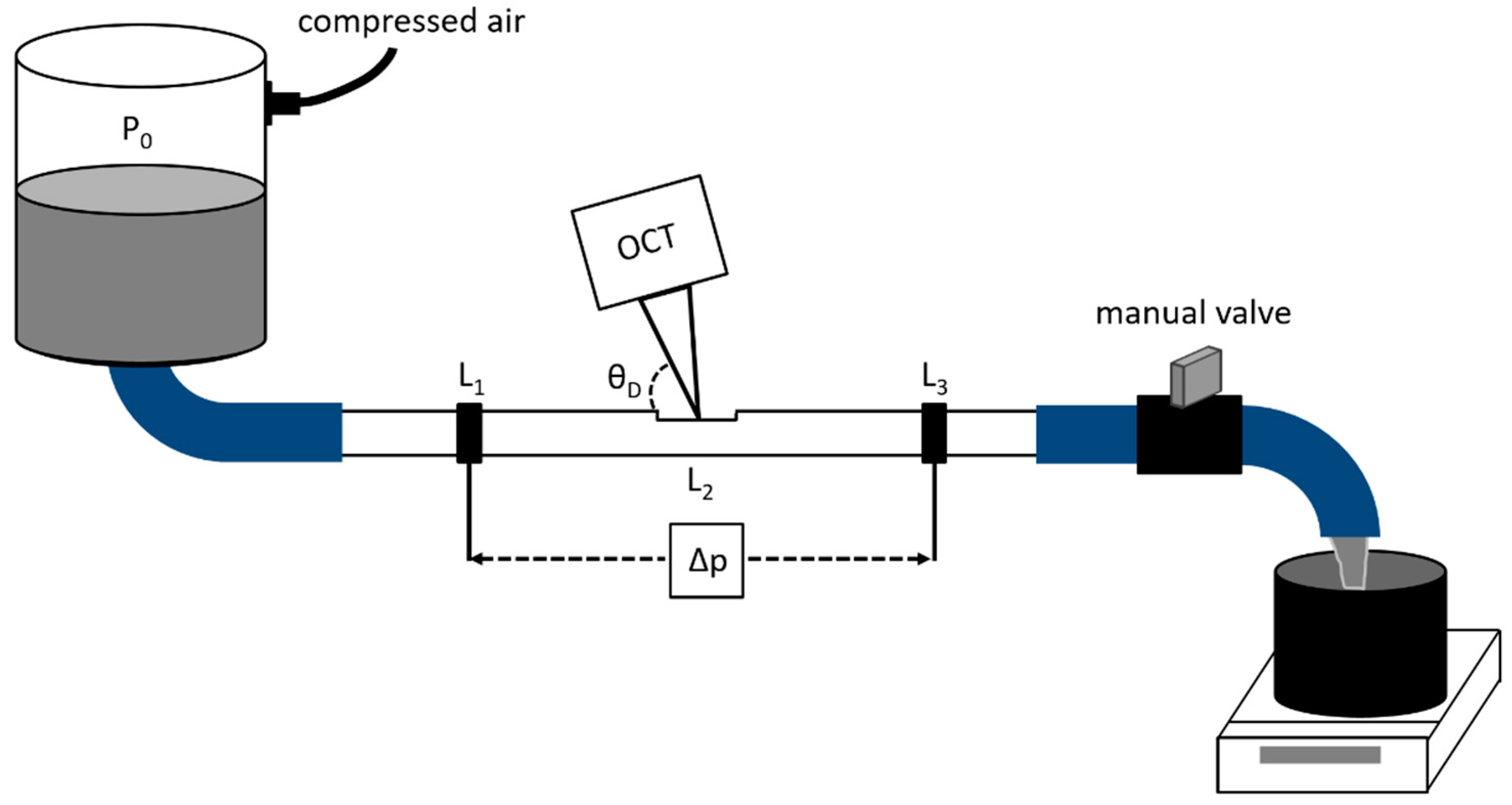
The experimental setup is shown in Figure 2. The measurement unit consisted of an optical grade glass pipe with an inner diameter of D = 8.6 mm. A container filled with the MFC suspension was connected to the pipe with a rubber hose and attached to a compressed air source via a pressure regulator. The suspension flow was controlled with both a manual valve after the glass pipe and the set overpressure in the container. The flow was is all cases both laminar and fully developed. The pressure gradient ∇P in the pipe was acquired with a differential pressure sensor (2051, Emerson Electric, St. Louis, MO, USA; the probes were located at the distance of L1 = 52D and L3 = 150D from the pipe inlet). The pressure gradient was used to calculate the wall shear stress = D∇P/4. For each flow rate, 50,000 DOCT A-scans were acquired at a distance of L2 = 110D from the pipe inlet. Here, a laboratory-built spectral domain DOCT device was used; the detailed device description can be found in refs. [24,25]. This device has an axial resolution of 0.9 µm in water. The submicron resolution was achieved by combining a custom OCT spectrometer (designed for the spectral region of 400–800 nm) with an ultra-broadband supercontinuum laser source (SuperK Extreme EXB-1, NKT Photonics, Birkerød, Denmark). The maximum scanning depth of the device is 365 µm in water, and the maximum scanning rate is 123 kHz. The accusracy of the used OCT setup has been verified in microfluidic flow conditions in ref. [25]. There the volumetric flow rate determined from the DOCT velocity profile deviated 6% from the set volumetric flow rate. The pipe rheometer configuration and the DOCT measurements are presented in more detail in ref. [10].
Figure 3 shows an example of the measured velocity and amplitude signals. Velocity data could be obtained, in the best case, up to 200 μm from the pipe wall, excluding the immediate vicinity of the wall. The closest point relative to the pipe wall having reliable velocity data was estimated to be 2 µm, below which the profiles were affected by the signal originating from the wall.
3. Results and Discussion
The velocity profiles obtained could be characterized in the following way. For the lowest flow rates, when the wall shear stress was below the yield stress τy = 3.4 Pa of the MFC suspension [10], the velocity profile corresponded to a pure plug flow in the whole pipe, excluding a yielding marginal wall layer of a few microns in thickness. When the wall shear stress exceeded the yield stress, the velocity profiles consisted of three distinctive parts (see Figure 3). In the outer (bulk) region, at the distances greater than 20 µm, the shear rate was small. In the region of 2–20 µm the velocity profile was rather steep and approached zero towards the wall. In the immediate vicinity of the wall (distance 0–2 µm), the velocity dropped abruptly to zero. The most natural explanation for the observed behavior of the velocity profile was a development of a consistency profile in the pipe, caused by wall depletion [26], when the distance from the wall was smaller than 20 µm.
The measured velocity profiles were fitted by the empirical formula
where y is the distance from the wall and , , and are free parameters. Parameter is the apparent shear rate at wall, and are the apparent slip velocities, and is the characteristic thickness of the (apparent) slip layer. The local viscosity of the suspension could then be calculated from the formula
where y is the distance from the pipe wall, , and is the local shear rate.
Outside the wall depletion layer (y > 20 µm), but still close to the wall (y < 200 µm), the shear rate and shear stress are approximately and , respectively. Figure 4 shows the viscosity of the MFC suspension in the bulk (y > 20 µm). Above its yield stress, the well-known shear thinning (power-law) behaviour of MFC suspensions is evident in Figure 4 (5–15 Pa). This behaviour is also typical for fibre suspensions and is believed to be due to adhesive contacts between the fibres that are broken by the shear forces when the shear rate increases [27,28]. As a result, the (floc) structure of the MFC suspension changes [29,30]. Notice, that close to and below the yield stress the viscosity values are large, and there are strong fluctuation in their values. Large values are due to the values of being close to zero when the suspension is non-yielded. The strong variation in the viscosity values is due to continuous break-up and recovery of the local network structure in the flow. Such fluctuations may be caused by small variations in shear history and a non-homogeneous floc structure of the sample suspension. This effect could be minimized by using longer measurement times.
Figure 4 shows that there is a narrow transition region between two power laws, which takes place when the shear stress is ca. 10 Pa. To our knowledge, this kind of viscosity behavior has not been reported earlier for MFC suspensions. Such abrupt change in the rheological behavior of the MFC suspension is likely to be related with a sudden structural change in the suspension, for example, in fibre orientation [31] and/or flocculation [28].
For the floc size analysis, 50 images consisting of 1000 successive A-scans were analysed for the amplitude signals. The analysed area was 100 µm long in the radial direction and started 20 µm from the wall to avoid the effect of the wall depletion layer on the results. The uneven OCT amplitude profile (see Figure 3) was eliminated from the images by scaling individual amplitude A-scans with an averaged A-scan amplitude profile. This correction removes all stationary intensity variations from original A-scans, and the remaining intensity variations are due to temporal differences in the local suspension properties (see Figure 5). A dominant factor causing most of these variations is the local concentration of the suspension. Due to different flow rates and scanning frequencies, the size of the analysed area varied in axial flow direction between 60 µm and 1.1 mm (pixel sizes in the axial flow direction thus varied between 0.06 µm and 1.1 µm). In order to make the analysis of different flow rates and their axial and radial floc sizes commensurate, all images were resized to the pixel size of 1.1 µm, using MATLAB’s (ver. 9.1.0.441655 R2016b, MathWorks, Natick, MA, USA) imresize routine, which performs a bicubic interpolation.
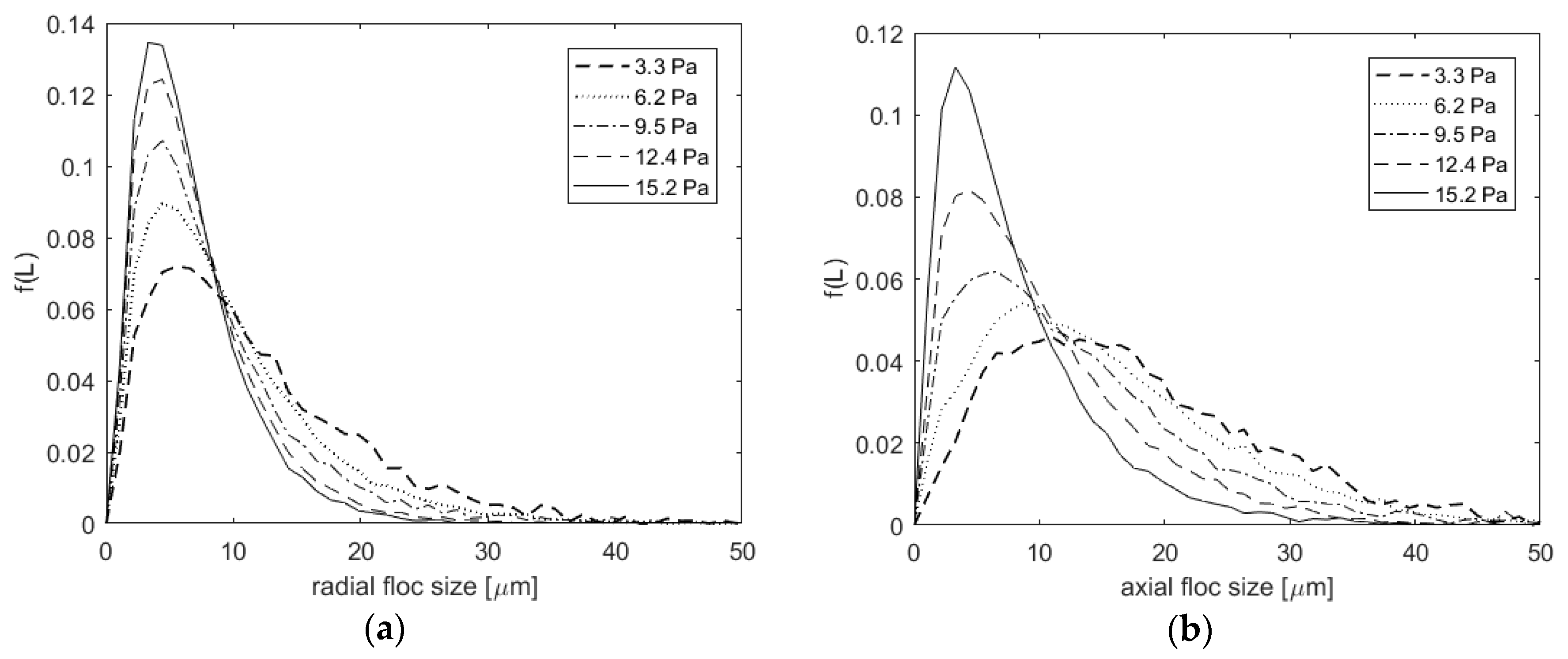
The floc size analysis was performed using the method presented in [8]. The OCT structural images were thresholded separately using the median of intensity. The (length-weighted) distribution of floc dimensions, in both radial and axial directions, was then computed for every image in the sequence as the run-length distributions (see Figure 6). The floc size distributions were log-normal, which are typical for fibers [32,33] and many other flocculating particles [34,35]. Determined distributions were finally averaged to obtain the length weighted average floc sizes.
Figure 7 shows the axial and radial floc size as a function of wall shear stress. Both floc sizes are seen to remain approximately constant below the yield stress of τy = 3.4 Pa. Above the yield stress, the both floc sizes decrease monotonically and become approximately equal at the highest wall shear stress of 15.2 Pa. Furthermore, the radial and axial floc size distributions are almost identical at the highest wall shear stress (see Figure 6). The above observations indicate that the suspension is finally well fluidized.
There appears to be an abrupt drop (see the arrow in Figure 7) in both radial and axial floc sizes at τw = 10 Pa, after which the floc size remains almost constant up to τw = 12 Pa. This sudden structural change coincides with the sudden drop in the viscosity of the suspension (see Figure 4). The number of data points is, however, rather limited, and additional experiments are needed to verify this interesting behavior.
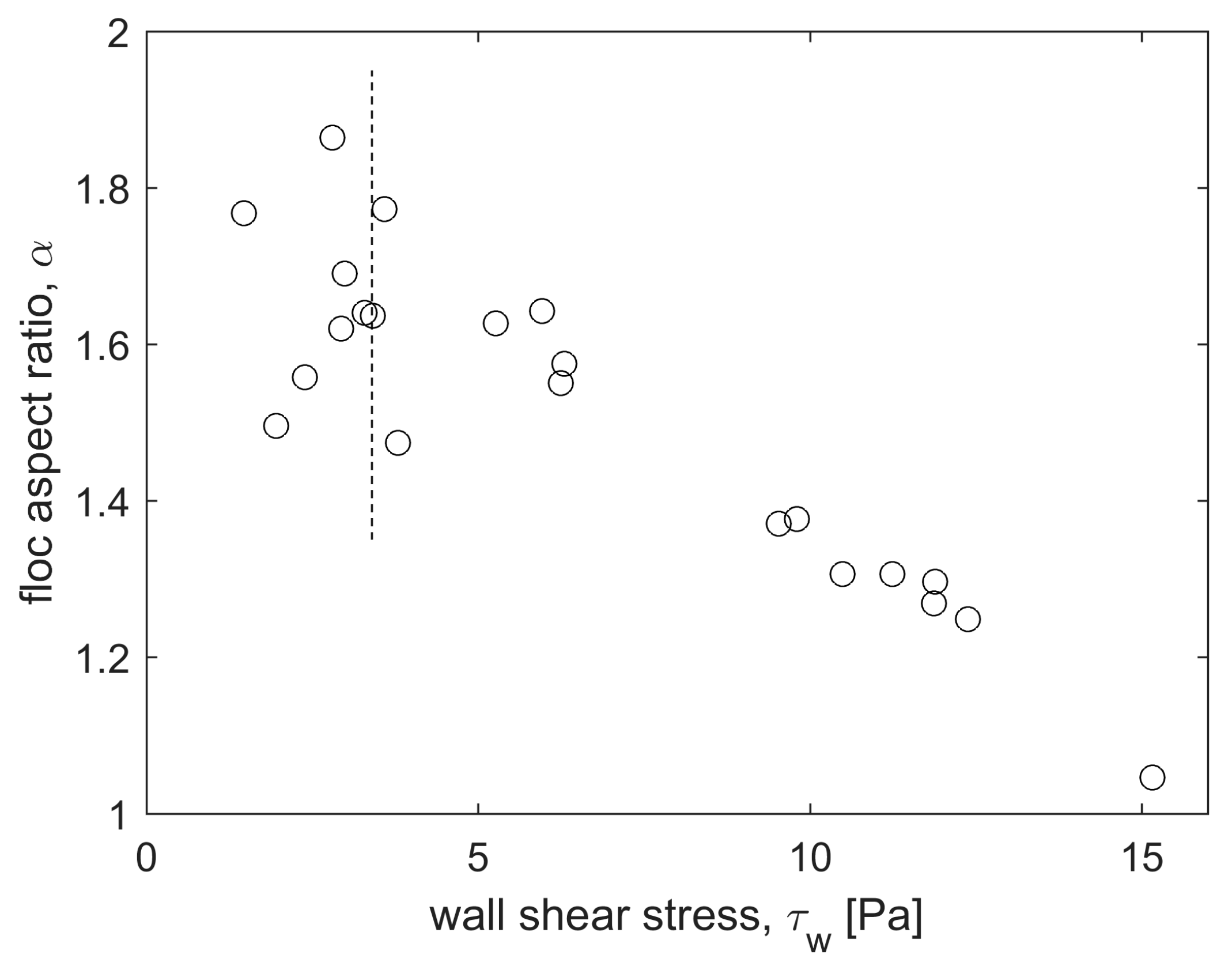
Figure 8 shows the floc aspect ratio α (axial size/radial size) as the function of the wall shear stress. We see from Figure 8 that the floc aspect ratio α varies a lot with the smallest wall shear rates, but it appears to stay approximately constant, α = 1.6, at least until wall shear stress of 6 Pa. The elongation of the MFC flocs (from spheres into prolates) has probably happened already during the constriction conditions of the flow of the suspension from the plastic container into the rubber hose [36]. Furthermore, the data in Figure 8 suggest that when the wall shear stress exceeds 6 Pa, the floc aspect ratio starts to decrease monotonically reaching approximately α ≈ 1 with the highest shear stress. Unfortunately, there are no measurement points in the wall shear stress range of 6–9 Pa, and thus the more accurate onset of this phenomenon remains unclear.
As pointed in [8], geometry gap dimensions and material may affect flocculation. Especially with small gaps, wall depletion may hinder the breakdown of the flocs, and the floc sizes can reach dimensions of the gap. Probably due to the rheometer geometry and the imaging setup, the floc size varied for an identical MFC suspension between 0.1–1 mm in [9], being in a completely different length scale when compared with the present study. Also, the dynamic behavior of flocculation was qualitatively very different when compared with our results for the pipe flow. During the rheometer measurements, the floc size usually increased until the yield stress was reached above which the floc size decreased with increasing shear stress.
While the number of flocculation studies with MFC is rather low, dynamics of flocculation and floc rupture of wood fibers and other materials has been studied extensively [37,38,39,40,41]. The observations on the flocculation and breaking mechanisms have varied a lot, but the relation between the floc size L and shear stress τ has typically been a power law
As we see from Figure 7, this is also the case here for the radial floc size Lr with β = 0.32. Depending on the floc breaking mechanism and inertial range, one can find in literature various values for β [38,42]. Similar values (β ~ 0.3) have been reported, for example, in [43,44]. The dynamics of the axial floc size La is more complicated; the slope for La is up to 6 Pa approximately the same as for Lr, but above 6 Pa it is twice as big. It is probable that the elongational forces due to the constriction conditions in the outflow from the container not only stretch, but also break flocs, when wall shear rate exceeds 6 Pa [45,46].
4. Conclusions
In this work, a sub-micron resolution optical coherence tomography device was used together with a pipe rheometer to analyze the rheology and flocculation dynamics of a 0.5% MFC suspension. The bulk behavior of the studied MFC suspension showed typical shear thinning (power-law) behavior in the interior part of the tube. This was reflected with a monotonously decreasing floc size when the shear stress exceeded the yield stress of the suspension. Here, the radial floc size followed a power law, while the dynamics of the axial floc size was more complicated.
The quantitative viscous behavior of the MFC suspension changed abruptly at the wall shear stress of 10 Pa, which is likely due to a sudden structural change of the suspension. Indeed, there appeared to be a simultaneous abrupt drop in both the radial and the axial floc sizes. The number of data points is, however, rather limited, and additional experiments are needed to verify this flocculation behavior.
The benefit of performing the rheological experiments in a real process geometry (pipe flow) was confirmed by comparing the flocculation results with earlier rheometer studies. While the flocculation behavior was consistent in the current study, the restricted geometries used in earlier studies have likely contributed to the observed intricate flocculation behavior.
As yet, there has been a lack of experimental techniques that would allow direct measurement of flows and internal structures of complex, opaque fluids especially in the immediate vicinity of the wall. OCT provides a remedy for this long-standing grievance by bringing excellent new possibilities for improving and extending the capabilities of existing rheological measurement devices and methods.
Author Contributions
J.L., and S.H. conceived and designed the experiments; J.L. performed the experiments; J.L. and A.I.K. analyzed the data; J.L., S.H. and A.I.K. wrote the manuscript; T.F. supervised the OCT-analysis and technology; A.I.K. supervised the rheological analysis.
Acknowledgments
Academy of Finland (project 288694) is gratefully acknowledged for supporting this work. We also want to thank senior research technician Ulla Salonen for the photograph of the MFC fibers (Figure 1), and senior scientist Panu Lahtinen for preparing the MFC.
Conflicts of Interest
The authors declare no conflict of interest.
References
- Isogai, A. Wood nanocelluloses: Fundamentals and applications as new bio-based nanomaterials. J. Wood Sci. 2013, 59, 449–459. [Google Scholar] [CrossRef]
- Klemm, D.; Kramer, F.; Moritz, S.; Lindström, T.; Ankerfors, M.; Gray, D.; Dorris, A. Nanocelluloses: A New Family of Nature-Based Materials. Angew. Chem. Int. Ed. 2011, 50, 5438–5466. [Google Scholar] [CrossRef] [PubMed]
- Moon, R.J.; Schueneman, G.T.; Simonsen, J. Overview of Cellulose Nanomaterials, Their Capabilities and Applications. JOM 2016, 68, 2383–2394. [Google Scholar] [CrossRef]
- Naderi, A.; Lindström, T. Rheological measurements on nanofibrillated cellulose systems: A science in progress. In Cellulose and Cellulose Derivatives: Synthesis, Modification and Applications; Mondal, M.I.H., Ed.; Nova Science Publishers: New York, NY, USA, 2015. [Google Scholar]
- Nazari, B.; Kumar, V.; Bousfield, D.W.; Toivakka, M. Rheology of cellulose nanofibers suspensions: Boundary driven flow. J. Rheol. 2016, 60, 1151–1159. [Google Scholar] [CrossRef]
- Kumar, V.; Nazari, B.; Bousfield, D.W.; Toivakka, M. Rheology of microfibrillated cellulose suspensions in pressure-driven flow. Appl. Rheol. 2016, 26, 43534. [Google Scholar] [CrossRef]
- Karppinen, A.; Saarinen, T.; Salmela, J.; Laukkanen, A.; Nuopponen, M.; Seppälä, J. Flocculation of microfibrillated cellulose in shear flow. Cellulose 2012, 19, 1807–1819. [Google Scholar] [CrossRef]
- Saarikoski, E.; Saarinen, T.; Salmela, J.; Seppälä, J. Flocculated flow of microfibrillated cellulose water suspensions: An imaging approach for characterisation of rheological behaviour. Cellulose 2012, 19, 647–659. [Google Scholar] [CrossRef]
- Saarinen, T.; Haavisto, S.; Sorvari, A.; Salmela, J.; Seppälä, J. The effect of wall depletion on the rheology of microfibrillated cellulose water suspensions by optical coherence tomography. Cellulose 2014, 21, 1261–1275. [Google Scholar] [CrossRef]
- Lauri, J.; Koponen, A.; Haavisto, S.; Czajkowski, J.; Fabritius, T. Analysis of rheology and wall depletion of microfibrillated cellulose suspension using optical coherence tomography. Cellulose 2017, 24, 4715–4728. [Google Scholar] [CrossRef]
- Swerin, A.; Ödberg, L.; Lindström, T. Deswelling of hardwood kraft pulp fibers by cationic polymers. Nord. Pulp. Pap. Res. J. 1990, 5, 188–196. [Google Scholar] [CrossRef]
- Huang, D.; Swanson, E.; Lin, C.; Schuman, J.; Stinson, W.; Chang, W.; Hee, M.; Flotte, T.; Gregory, K.; Puliafito, C.; et al. Optical coherence tomography. Science 1991, 254, 1178–1181. [Google Scholar] [CrossRef] [PubMed]
- Zhao, Y.; Chen, Z.; Saxer, C.; Xiang, S.; de Boer, J.F.; Nelson, J.S. Phase-resolved optical coherence tomography and optical Doppler tomography for imaging blood flow in human skin with fast scanning speed and high velocity sensitivity. Opt. Lett. 2000, 25, 114–116. [Google Scholar] [CrossRef] [PubMed]
- Wang, X.J.; Milner, T.E.; Nelson, J.S. Characterization of fluid flow velocity by optical Doppler tomography. Opt. Lett. 1995, 20, 1337–1339. [Google Scholar] [CrossRef] [PubMed]
- Wang, R.K. High-resolution visualization of fluid dynamics with Doppler optical coherence tomography. Meas. Sci. Technol. 2004, 15, 725–733. [Google Scholar] [CrossRef]
- Bonesi, M.; Churmakov, D.; Meglinski, I. Study of flow dynamics in complex vessels using Doppler optical coherence tomography. Meas. Sci. Technol. 2007, 18, 3279–3286. [Google Scholar] [CrossRef]
- Lauri, J.; Bykov, A.V.; Priezzhev, A.V.; Myllylä, R. Experimental study of the multiple scattering effect on the flow velocity profiles measured in Intralipid phantoms by DOCT. Laser Phys. 2011, 21, 813–817. [Google Scholar] [CrossRef]
- Haavisto, S.; Salmela, J.; Koponen, A. Accurate velocity measurements of boundary-layer flows using Doppler optical coherence tomography. Exp. Fluids 2015, 56, 96. [Google Scholar] [CrossRef]
- Malm, A.V.; Waigh, T.A. Elastic turbulence in entangled semi-dilute DNA solutions measured with optical coherence tomography velocimetry. Sci. Rep. 2017, 7, 1186. [Google Scholar] [CrossRef] [PubMed]
- Harvey, M.; Waigh, T.A. Optical coherence tomography velocimetry in controlled shear flow. Phys. Rev. E 2011, 83, 031502. [Google Scholar] [CrossRef] [PubMed]
- Jaradat, S.; Harvey, M.; Waigh, T.A. Shear-banding in polyacrylamide solutions revealed via optical coherence tomography velocimetry. Soft Matter 2012, 8, 11677–11686. [Google Scholar] [CrossRef]
- Lauri, J.; Bykov, A.V.; Myllyla, R. Determination of suspension viscosity from the flow velocity profile measured by Doppler Optical Coherence Tomography. Photonics Lett. Pol. 2011, 3, 82–84. [Google Scholar] [CrossRef]
- Haavisto, S.; Salmela, J.; Jäsberg, A.; Saarinen, T.; Karppinen, A.; Koponen, A. Rheological characterization of microfibrillated cellulose suspension using optical coherence tomography. TAPPI J. 2015, 14, 291–302. [Google Scholar]
- Czajkowski, J.; Vilmi, P.; Lauri, J.; Sliz, R.; Fabritius, T.; Myllyla, R. Characterization of ink-jet printed RGB color filters with spectral domain optical coherence tomography. In Proceedings of the SPIE 8493, Interferometry XVI: Techniques and Analysis, San Diego, CA, USA, 16 July 2012; pp. 849308–849308-7. [Google Scholar] [CrossRef]
- Lauri, J.; Czajkowski, J.; Myllylä, R.; Fabritius, T. Measuring flow dynamics in a microfluidic chip using optical coherence tomography with 1 µm axial resolution. Flow Meas. Instrum. 2015, 43, 1–5. [Google Scholar] [CrossRef]
- Barnes, H.A. A review of the slip (wall depletion) of polymer solutions, emulsions and particle suspensions in viscometers: Its cause, character, and cure. J. Non Newton. Fluid Mech. 1995, 56, 221–251. [Google Scholar] [CrossRef]
- Petrich, M.P.; Koch, D.L.; Cohen, C. An experimental determination of the stress-microstructure relationship in semi-concentrated fiber suspensions. J. Non Newton. Fluid Mech. 2000, 95, 101–133. [Google Scholar] [CrossRef]
- Bounoua, S.; Lemaire, E.; Férec, J.; Ausias, G.; Kuzhir, P. Shear-thinning in concentrated rigid fiber suspensions: Aggregation induced by adhesive interactions. J. Rheol. 2016, 60, 1279–1300. [Google Scholar] [CrossRef]
- Agoda-Tandjawa, G.; Durand, S.; Berot, S.; Blassel, C.; Gaillard, C.; Garnier, C.; Doublier, J.-L. Rheological characterization of microfibrillated cellulose suspensions after freezing. Carbohydr. Polym. 2010, 80, 677–686. [Google Scholar] [CrossRef]
- Iotti, M.; Gregersen, Ø.W.; Moe, S.; Lenes, M. Rheological Studies of Microfibrillar Cellulose Water Dispersions. J. Polym. Environ. 2011, 19, 137–145. [Google Scholar] [CrossRef]
- Mykhaylyk, O.O.; Warren, N.J.; Parnell, A.J.; Pfeifer, G.; Laeuger, J. Applications of shear-induced polarized light imaging (SIPLI) technique for mechano-optical rheology of polymers and soft matter materials. J. Polym. Sci. Pol. Phys. 2016, 54, 2151–2170. [Google Scholar] [CrossRef]
- Hourani, M.J. Fiber flocculation in pulp suspension flow: Part 2. Experimental results. TAPPI J. 1988, 71, 186–189. [Google Scholar]
- Hourani, M.J. Fiber flocculation in pulp suspension: Part 1. Theoretical model. TAPPI J. 1988, 71, 115–118. [Google Scholar]
- Coufort, C.; Dumas, C.; Bouyer, D.; Liné, A. Analysis of floc size distributions in a mixing tank. Chem. Eng. Process. Process Intensif. 2008, 47, 287–294. [Google Scholar] [CrossRef]
- Shin, J.H.; Son, M.; Lee, G. Stochastic Flocculation Model for Cohesive Sediment Suspended in Water. Water 2015, 7, 2527–2541. [Google Scholar] [CrossRef]
- Kerekes, R.J. Pulp floc behaviour in entry flow to constrictions [Paper industry]. TAPPI J. 1983, 66, 88–91. [Google Scholar]
- Thomas, D.N.; Judd, S.J.; Fawcett, N. Flocculation modelling: A review. Water Res. 1999, 33, 1579–1592. [Google Scholar] [CrossRef]
- Jarvis, P.; Jefferson, B.; Gregory, J.; Parsons, S.A. A review of floc strength and breakage. Water Res. 2005, 39, 3121–3137. [Google Scholar] [CrossRef] [PubMed] [Green Version]
- Cui, H.; Grace, J.R. Flow of pulp fibre suspension and slurries: A review. Int. J. Multiph. Flow 2007, 33, 921–934. [Google Scholar] [CrossRef]
- Keshtkar, M.; Heuzey, M.C.; Carreau, P.J. Rheological behavior of fiber-filled model suspensions: Effect of fiber flexibility. J. Rheol. 2009, 53, 631–650. [Google Scholar] [CrossRef]
- Son, M.; Hsu, T.-J. The effect of variable yield strength and variable fractal dimension on flocculation of cohesive sediment. Water Res. 2009, 43, 3582–3592. [Google Scholar] [CrossRef] [PubMed]
- François, R.J. Strength of aluminium hydroxide flocs. Water Res. 1987, 21, 1023–1030. [Google Scholar] [CrossRef]
- Sonntag, R.C.; Russel, W.B. Structure and breakup of flocs subjected to fluid stresses. J. Colloid Interface Sci. 1986, 113, 399–413. [Google Scholar] [CrossRef]
- Biggs, C.A.; Lant, P.A. Activated sludge flocculation: On-line determination of floc size and the effect of shear. Water Res. 2000, 34, 2542–2550. [Google Scholar] [CrossRef]
- Hubbe, M. Flocculation and redispersion of cellulosic fiber suspensions: A review of effects of hydrodynamic shear and polyelectrolytes. BioResources 2007, 2, 296–331. [Google Scholar]
- Blaser, S. Break-up of flocs in contraction and swirling flows. Colloid Surface A 2000, 166, 215–223. [Google Scholar] [CrossRef]
Figure 1.
An image of the microfibrillated cellulose (MFC) used in this study. The distributions of length and width are very broad.
Figure 1.
An image of the microfibrillated cellulose (MFC) used in this study. The distributions of length and width are very broad.
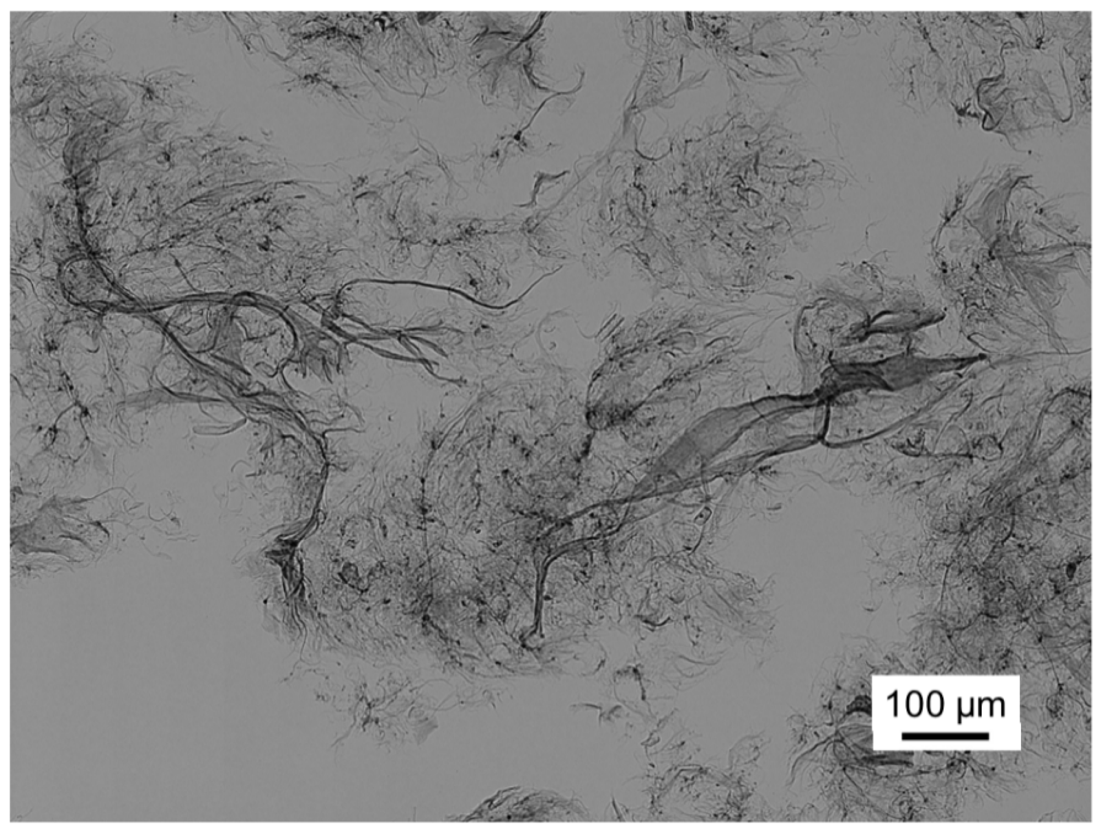
Figure 2.
A schematic of the experimental setup. The optical coherence tomography (OCT) measurement is performed for a fully developed laminar flow of the MFC suspension in a straight glass tube with a diameter of D = 8.6 mm. The pressure measurement taps are located at L1 = 52D and L3 = 150D from the pipe inlet. The OCT is located at L2 = 110D from the pipe inlet. A computer-controlled scale is used for the mass flow rate measurements.

Figure 3.
An example of a measured flow velocity profile (dots) together with the corresponding OCT amplitude signal (solid line) at the flow rate of 158 mL/min. The peak in the amplitude signal due to the tube wall is marked with an arrow.
Figure 3.
An example of a measured flow velocity profile (dots) together with the corresponding OCT amplitude signal (solid line) at the flow rate of 158 mL/min. The peak in the amplitude signal due to the tube wall is marked with an arrow.
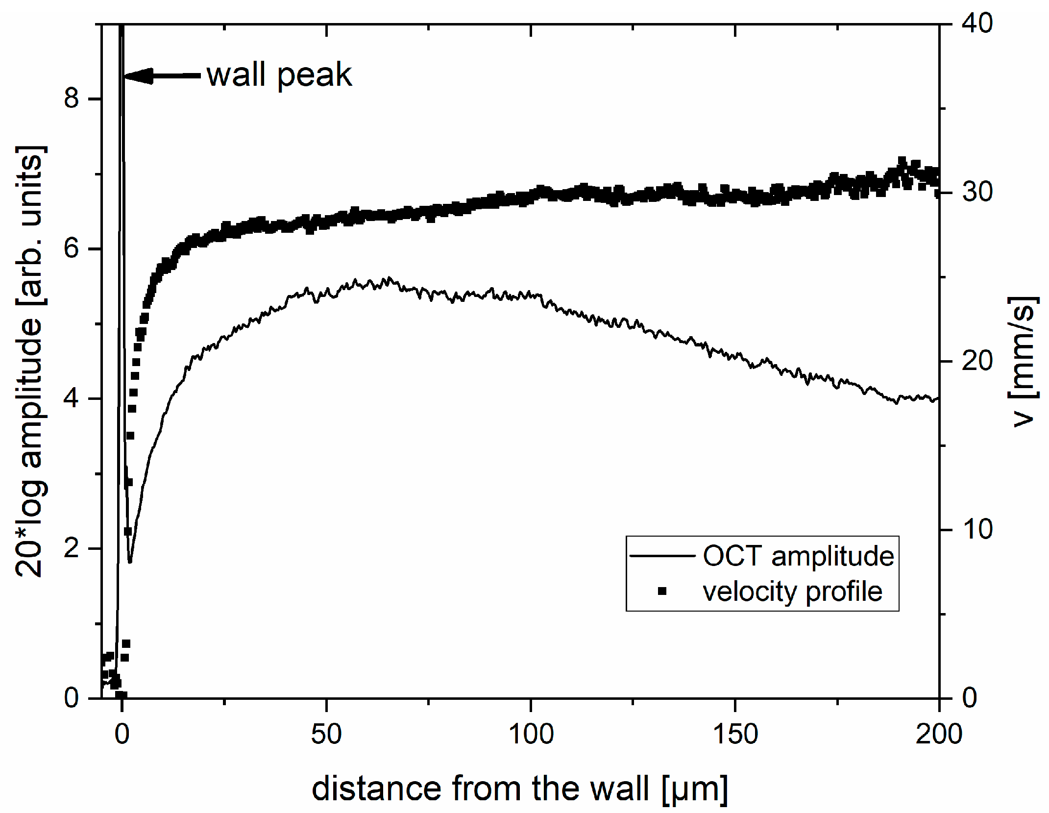
Figure 4.
Viscosity as a function of shear stress. The viscosities have been calculated with Equation (2). The dashed and solid lines show fits of the power law μ = A to the two sets of the pipe flow data. The dash-dotted line shows the yield stress τy = 3.4 Pa of the MFC.
Figure 4.
Viscosity as a function of shear stress. The viscosities have been calculated with Equation (2). The dashed and solid lines show fits of the power law μ = A to the two sets of the pipe flow data. The dash-dotted line shows the yield stress τy = 3.4 Pa of the MFC.
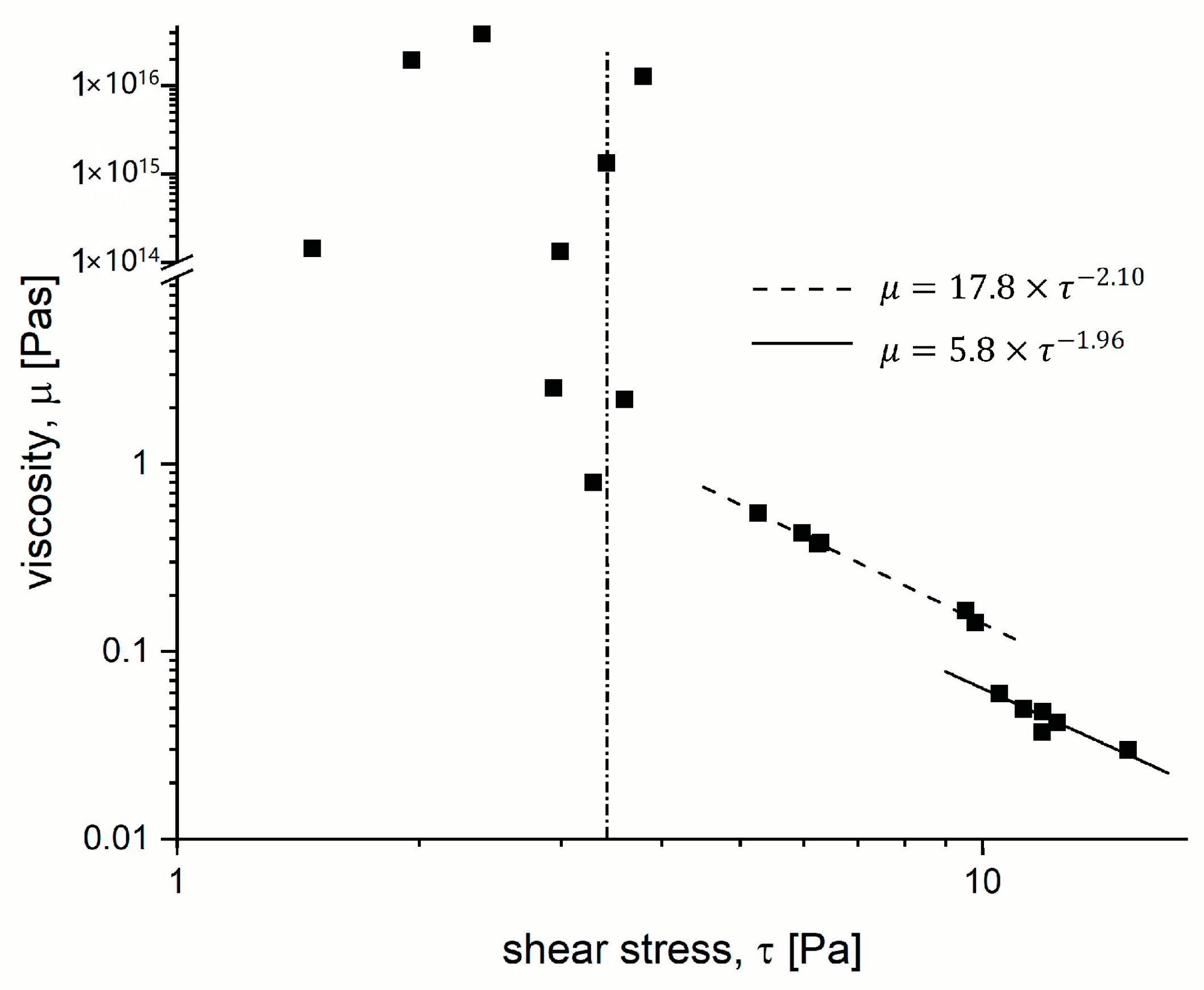
Figure 5.
Intensity-corrected structural OCT images composed of successive A-scans of the suspension with the wall shear stress and scan count of (a) 3.8 Pa, 1000, and (b) 11.2 Pa, 430, respectively. Bright color indicates high and dark color low MFC consistency. Image size is 120 µm × 290 µm. The pipe wall is on the top of the image and the flow direction is from left to right. The arrows show the axial and radial directions.
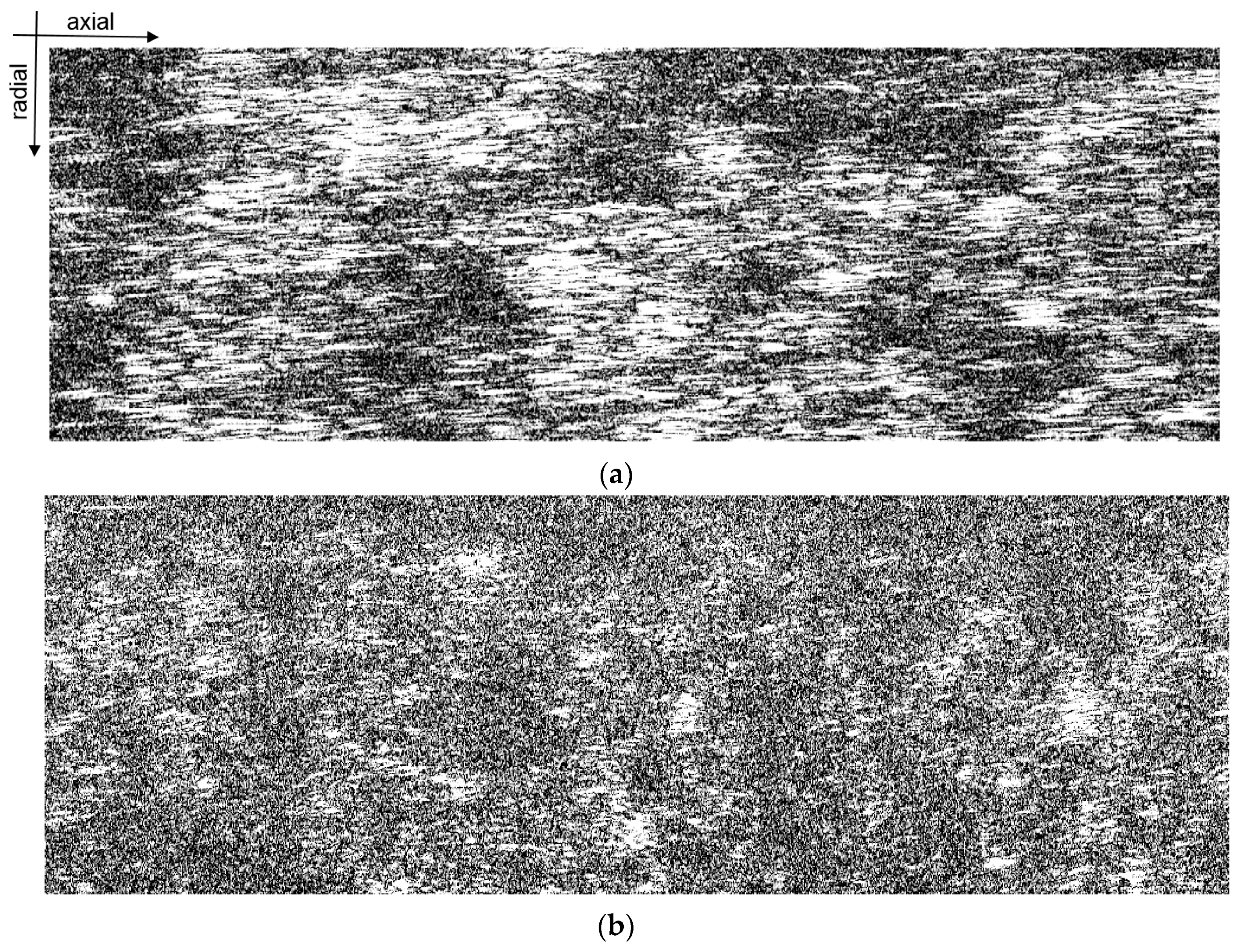
Figure 6.
(a) Radial and (b) axial floc size distributions calculated with the run-length method [8]. Both axial and radial floc sizes decrease with an increasing wall shear stress.
Figure 6.
(a) Radial and (b) axial floc size distributions calculated with the run-length method [8]. Both axial and radial floc sizes decrease with an increasing wall shear stress.

Figure 7.
The radial and axial floc size as a function of wall shear stress. The floc sizes remain approximately constant until wall shear stress exceeds the yield stress τy = 3.4 Pa (dashed line). The radial floc size Lr appears to follow a power law (solid line). The dynamics of the axial floc size is more complicated. The arrow shows the abrupt drop of the axial floc size at τw =10 Pa.
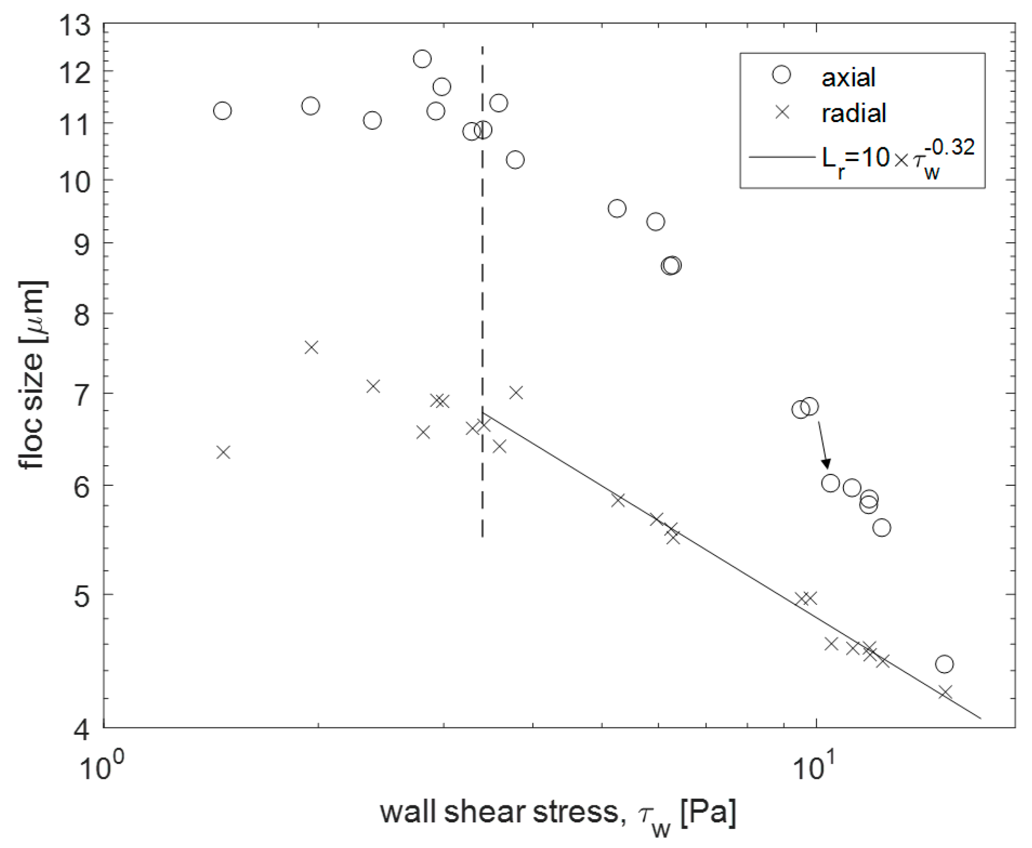
Figure 8.
Floc aspect ratio (axial size/radial size) as a function of wall shear stress. The yield stress τy = 3.4 Pa is shown with a vertical dashed line.
Figure 8.
Floc aspect ratio (axial size/radial size) as a function of wall shear stress. The yield stress τy = 3.4 Pa is shown with a vertical dashed line.
© 2018 by the authors. Licensee MDPI, Basel, Switzerland. This article is an open access article distributed under the terms and conditions of the Creative Commons Attribution (CC BY) license (http://creativecommons.org/licenses/by/4.0/).
Share and Cite
MDPI and ACS Style
Koponen, A.I.; Lauri, J.; Haavisto, S.; Fabritius, T. Rheological and Flocculation Analysis of Microfibrillated Cellulose Suspension Using Optical Coherence Tomography. Appl. Sci. 2018, 8, 755. https://doi.org/10.3390/app8050755
AMA Style
Koponen AI, Lauri J, Haavisto S, Fabritius T. Rheological and Flocculation Analysis of Microfibrillated Cellulose Suspension Using Optical Coherence Tomography. Applied Sciences. 2018; 8(5):755. https://doi.org/10.3390/app8050755
Chicago/Turabian StyleKoponen, Antti I., Janne Lauri, Sanna Haavisto, and Tapio Fabritius. 2018. "Rheological and Flocculation Analysis of Microfibrillated Cellulose Suspension Using Optical Coherence Tomography" Applied Sciences 8, no. 5: 755. https://doi.org/10.3390/app8050755
Note that from the first issue of 2016, this journal uses article numbers instead of page numbers. See further details here.