Algorithm for Virtual Aggregates’ Reconstitution Based on Image Processing and Discrete-Element Modeling


1
School of Computer Engineering, Nanjing Institute of Technology, Nanjing 211167, China
2
School of Transportation, Southeast University, 2 Sipailou, Nanjing 210096, China
3
School of Engineering and Architecture, Nanjing Institute of Technology, Nanjing 211167, China
*
Author to whom correspondence should be addressed.
Appl. Sci. 2018, 8(5), 738; https://doi.org/10.3390/app8050738
Submission received: 15 February 2018
/
Revised: 9 April 2018
/
Accepted: 3 May 2018
/
Published: 7 May 2018
(This article belongs to the Special Issue Achievements and Prospects of Functional Pavement: Materials and Structures)
Abstract
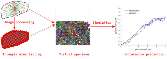
:Based on the Aggregate Imaging Measurement System (AIMS) and the Particle Flow Code in Two Dimensions (PFC2D), an algorithm for modeling two-dimensional virtual aggregates was proposed in this study. To develop the virtual particles precisely, the realistic shapes of the aggregates were captured by the AIMS firstly. The shape images were then processed, and the morphological characteristics of aggregates were quantified by the angularity index. By dividing the particle irregular shape into many triangle areas and adjusting the positions of the generated balls via coordinate systems’ conversion within PFC2D, the virtual particles could be reconstructed accurately. By calculating the mapping area, the gradations in two-dimensions could be determined. Controlled by two variables (μ_1 and μ_2), which were drawn from the uniform distribution (0, 1), the virtual particles forming the specimens could be developed with random sizes and angular shapes. In the end, the rebuilt model of the SMA-13 aggregate skeleton was verified by the virtual penetration tests. The results indicated that the proposed algorithm can not only model the realistic particle shape and gradations precisely, but also predict its mechanical behavior well.
1. Introduction
As the basis materials within the asphalt mixture, coarse aggregates are widely used in asphalt pavements, which form the main skeleton of the total structure. It has been highlighted by many researchers that the aggregates’ shape has a significant impact on controlling the mechanical properties of the asphalt mixtures [1,2,3]. Tests conducted by Campen and Smith [4] showed that the stability of hot-mix asphalt (HMA) concrete could be improved obviously by using crushed aggregates instead of rounded particles. Similar results were shown by Kandhal and Parker [5], that the HMA mixtures consisting of excessive flat and elongated aggregate particles tended to break down, affecting the mix durability. The fatigue performance of the asphalt mixture was also affected by the particles’ roundness and angularity, concluded based on Cheung and Dawson’s research [6]. In their studies, with the angularity increasing, the ultimate shear strength increased, and permanent deformation decreased, respectively. Thus, it is strongly recommended to use the complex angular particles to improve the grains’ interlocking and packing effectively.
However, it is really difficult and time-consuming to reveal the shape influences of coarse aggregates just by laboratory tests due to the appropriate definition of the morphological characteristics and the following shape acquisition, which is the basis to guarantee the results [7,8]. The discrete-element method (DEM) was proposed by the Cundall [9] firstly, and then, a software program named Particle Flow Code (PFC) was developed to help the mechanical calculation of heterogeneous materials, which has been widely used in many fields [10,11,12]. As the basic calculation elements, the balls in the software (PFC2D, Itasca Consulting Group: Minneapolis, USA) are all round shaped without any angular shape, which is not consistent with the realistic particles in pavement construction. Therefore, prior to numerical simulation, it is important to rebuild the realistic particle shape, which will influence the simulation results obviously [13,14,15]. Many modeling methods have been proposed within PFC to characterize the shape features by some researchers. Zhang et al. [16] regarded the aggregate particles as hexahedrons, pentahedrons and tetrahedrons within PFC, respectively. Then, the equal-radius balls were arranged regularly within the particles and were defined as a rigid body. CPA (Computerized Particle Analysis) was utilized to help develop the virtual shape within PFC by Stahl and Konietzky [17]. The input index, known as the grain-shape coefficient, was used to redefine the particle contour. Then, numerical particles were reconstructed by filling the redefined area with balls. Huang [18] reconstructed 3D ballast particles with three images (top, side and front) of the particles with the help of the image processing technology. Similar methods can also be found in the works of Liu and You [19,20], Tutumluer et al. [21] and Dondi and Vignali [22,23,24], as well. Most of the existing modeling methods can only model the shape roughly with excessive simplification. Although some virtual models were rebuilt precisely by X-ray scanning, the angular shape could not be quantified precisely [25,26,27,28,29]. Liu scanned the particles and rebuilt their virtual shapes according to the acquired images [30,31]. In their studies, the stl-format file were developed, which can reflect the shapes of aggregates precisely. By the designed routine, the virtual particles in three dimensions were developed successfully with enough balls filled. However, their methods can only model the realistic shapes, but cannot evaluate the shape properties of mixtures by a specific index. Therefore, the simulation accuracy mainly depends on the samples’ selection and cannot model the material heterogeneity well. Compared to X-ray scanning, the Aggregate Imaging Measurement System (AIMS) apparatus is a promising way for performing particle shape modeling and has been utilized gradually in material analyses [32]. It can capture the morphological characteristics of aggregates and quantifies the shape properties by some design indices such as the angularity index, texture index, size, and so on. However, this apparatus is mainly used for pavement skid resistance measurements nowadays [33,34,35]. More uses of it should be explored, especially combined with other technologies.
The objective of this study is to propose an algorithm for the virtual aggregates’ reconstitution based on the Discrete-Element Method (DEM). To achieve this, the AIMS apparatus with the image processing technology were utilized before the simulations. Then, an innovative method for developing the virtual particles and gradations was proposed precisely. In the end, based on the virtual penetration tests, the precision of the developed models was verified. The relevant issues include: capturing the shape image of particles by AIMS; processing the captured images and measuring their angularity index; modeling the virtual particles with different sizes and shapes; modeling the virtual gradations of specimens; developing the virtual penetration tests to predict and evaluate the performance of coarse aggregates.
2. Image Preprocessing and Shape Measurement
Prior to the virtual particles’ reconstitution, several steps were performed that could provide the proposed algorithm with the fundamental data. Firstly, enough aggregate particles were selected and were scanned by the AIMS to obtain their shape image and the angularity index. The particles were put in the turntable of the AIMS and were rotated slowly to go through the scanning area. A digital camera above the particles was utilized to capture the image of the maximum section from the top side. Then, the original images of the particles were converted to the binary ones within the MATLAB routine as shown in Figure 1. As shown, two forms of binary images were acquired via the image processing technology including the shape (Figure 1a) and its contour (Figure 1b).
Due to the size differences between the binary images and realistic particles, the processed images should be scaled back based on the actual ones. Because the binary images consisted of pixels only, the sizes were represented by the pixel number at different directions in the images rather than the actual length. In this proposed method, the relationship between the actual length and “pixel length” were quantified by uniform standards as one pixel equal to 0.005 mm. After this standard was developed, based on the actual particle size, the required reduction scale of binary images could be calculated to match the actual size, as shown in Table 1. Furthermore, after the images’ adjustment completed, the actual area of various particles was measured by the ImagePro software. The black area of the shape image in Figure 1a could be distinguished within the software, and the corresponding area was calculated and stored as shown in Table 1, as well.
Although there was an original coordinate system after image processing, another two coordinate systems were introduced in this proposed method to help the virtual particles’ reconstitution further, including the local coordinate system and global coordinate system. The local one will be introduced in the algorithm part, while the global one is developed as the following. It is necessary to develop a uniform global coordinate system for all particles because the original coordinate system in each image was not the same at all. The central position of each particle was defined firstly as shown in Equation (1):
where , are the X- and Y-coordinate values of the particle central position, respectively, in the original coordinate system; n is the total number of pixels in Figure 1b; , are the X- and Y-coordinate values of the i-th pixel in Figure 1b in the original coordinate system.
The original coordinate system of each image was converted to the uniform global coordinate system by setting the central positions as the new origin of the coordinates, and the adjustments of the original coordinate are summarized as shown in Table 2. It is noted that the data in Table 1 and Table 2 are only a part of the total virtual particles limited by space. The data shown were utilized to illustrate the preparation procedure.
3. Image Preprocessing and Shape Measurement
3.1. Triangle Area Divisions
As the independent element for calculation, the ball within PFC2D should be generated with a specific coordinate value. However, it is very hard to fill the particle shape area with balls directly because of the shape complexity, which prevents precise virtual particle modelling. The proposed algorithm converted the irregular particle shape into several triangles to make it easier to fill the required area with balls. The algorithm is illustrated as follows:
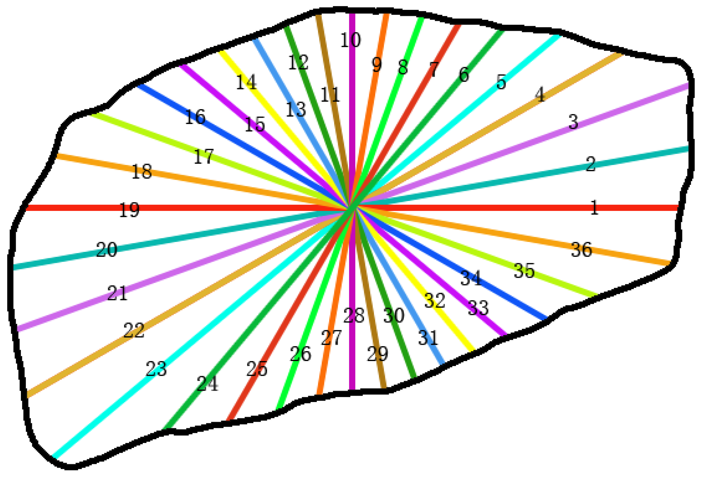
After the shape contour (Figure 1b) was scaled back, its irregular shape was divided into 36 triangle areas firstly, as shown in Figure 2. Measuring lines were drawn every 10 degrees by a user-defined routine based on MATLAB. They were drawn from the central position to the shape contour. Each triangle could represent a part of the shape area approximately. Then, the lengths of 36 lines were measured respectively by the routine. It is noted that the measuring lines in Figure 2 are not true lines, but a routine developed within MATLAB to measure the distance from the central position to the contour along the designed directions. The modelling precision and efficiency are definitely influenced by the number of divided triangles. As shown in Figure 2, with more triangles divided, the boundary of the virtual particle can have better accordance with the realistic one, but needs more complex routines for length measurements, which means more time consumption. To balance the simulation precision and efficiency, 36 triangle divisions were determined finally and were thought as the best after many tries.
3.2. Filling Area Judgments
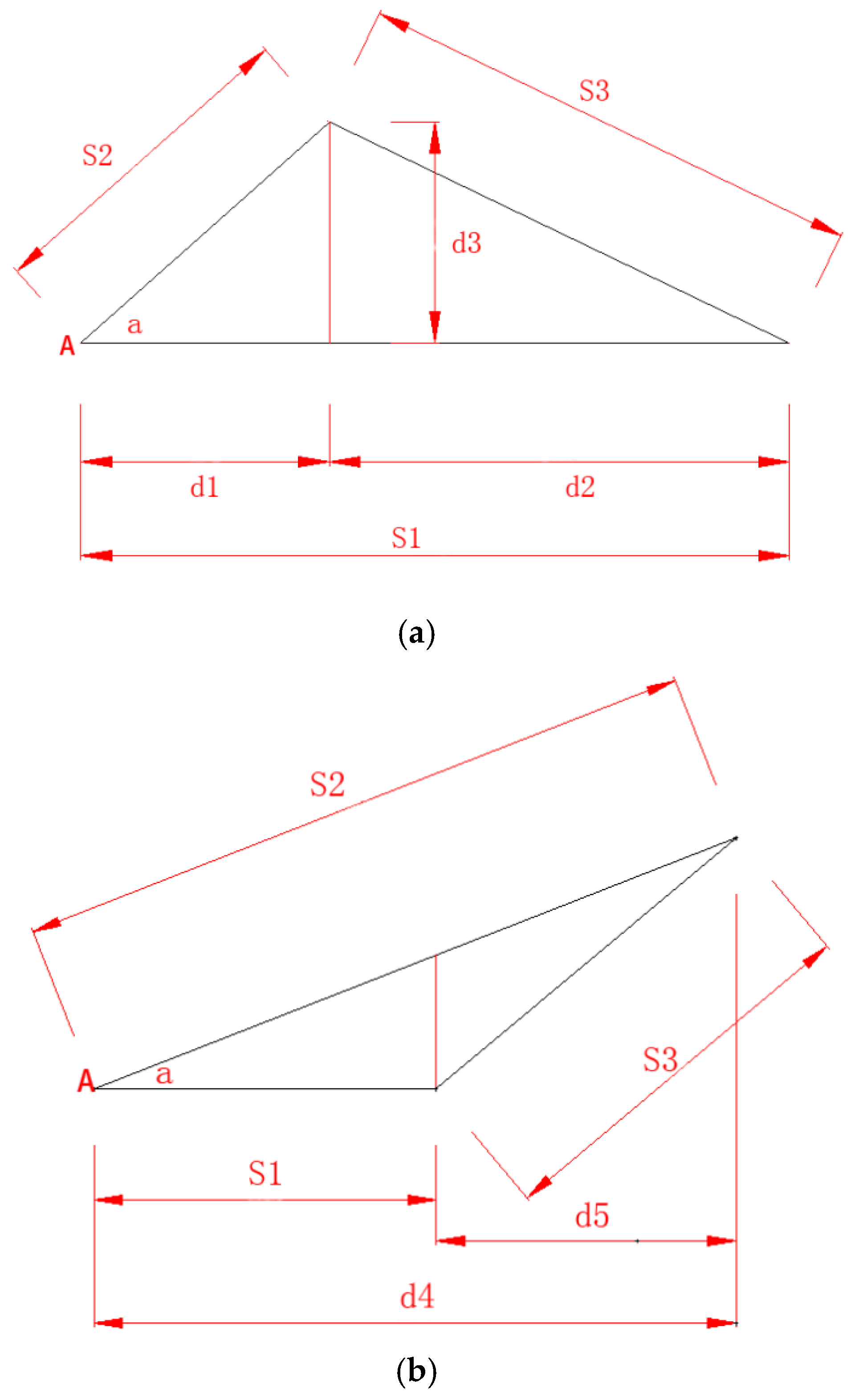
By labelling the lines with numbers increasing counter-clockwise as shown in Figure 2, the divided triangles could fall into two categories. One is that the top side of the triangle is longer than the bottom side; another is that the top one is shorter than the bottom one, as shown in Figure 3. The top side is always labelled with a larger number compared to the bottom side in one triangle. and are known quantities based on the former measurement in Figure 3, and “a” represents the included angle between two adjacent measuring lines with a magnitude of 10 degrees. , , , and were calculated as shown in Equation (2).
When (Figure 3a), the algorithm for filling the triangle area with balls by PFC2D was conducted as following:
- ①Start the ball generation from Point A with the coordinate of (0, 0);
- ②Determine the variable . It is calculated as the following equation:where is the X-coordinate of the next column of balls that will be generated; is the X-coordinate of the former column of balls that has been generated; is the radius of the filled balls.
- ③Determine the variable h, calculated as shown in Equation (4):where h is the required height of the next column of balls; the others are the same as the former.
- ④Generate uniform balls with coordinates of (, 0), (, ), (, ), (, ) … until the Y-coordinate exceeds h;
- ⑤Start to generate the next column of balls by cycling from Steps 2–4 until the X-coordinate exceeds .
When > (Figure 3b), the algorithm is conducted as follows:
- ①Start the ball generation from Point A with the coordinate of (0,0);
- ②Determine the variable . It is calculated as Equation (3):
- ③Determine the variable , calculated as shown in Equations (5) and (6):where is the required height of the next column of balls; the others are the same as the former.where is the required height of the next column of balls; is the lower limit of the column height when exceeds ; the others are the same as the former;
- ④When , generate uniform balls with coordinates of (, 0), (, 2 rad), (, 4 rad), (, 6 rad) … until the Y-coordinate exceeds ; when , generate uniform balls with the coordinates of (, ), (, ), (, ), (, ) … until the Y-coordinate exceeds ;
- ⑤Start to generate the next column of balls by cycling from Step 2–4 until the X-coordinate exceeds .
3.3. Coordinate Systems’ Conversion
By the proposed algorithm, the various triangle areas within the particle images could be filled with uniformly-arranged balls successfully. However, when combining all of the triangles to form the whole virtual particle, it is necessary to calibrate the coordinate value from the local coordinate system to the global one. The relationships between the two coordinate systems are shown in Figure 4. The X- and Y-coordinate of each filled ball should be adjusted based on Equation (7).
where and are the X-, Y-coordinates in the local coordinate system of the triangles, respectively; and are the X-, Y-coordinates in the global coordinate system of the particles, respectively; is the angle between the bottom side of the triangle () and the X-axis.
It is noted that two different coordinate systems were used in the modeling process. The local coordinate values represented the relative positions of balls in the virtual particles, while the global coordinate values represented relative positions of balls in the virtual container. When developing the single particle, the local coordinate systems were utilized to fill the irregular area with arranged balls. After that, the positions of all the virtual particles were converted to the global one so that the numerous virtual particles could be distributed within the designed area to form the whole mixtures. After the coordinates were calibrated, the virtual particles could be rebuilt as shown in Figure 5. As shown, the inner area of the virtual particles was filled with balls gradually after each triangle area was processed based on the proposed algorithm. However, although the irregular shapes of the particles were divided into several triangles, the side of (Figure 3) could only match the actual shape contour similarly. The shape modeling was not precise enough. Therefore, further improvements were made by modeling the shape contour firstly and then filling the inner area of the shape contour with balls by the former algorithm, as shown in Figure 5. The shape contour in Figure 1b was processed by a user-defined routine to read and store the pixel locations of the images. The black pixels were distinguished. Then, a threshold value of 0.005 was selected to filter the redundant black pixels such that the adjacent black pixels within a distance of 0.005 could be ignored and the others retained. By importing the locations of the retained pixels into PFC2D, the balls could be generated in the shape contour, as shown in Figure 5. Then, the whole particle was filled with balls by triangle area filling in the end. Based on the scanning images and with the help of the proposed algorithm, aggregate particles varying in size and shape were reconstructed as shown in Figure 6.
4. Algorithm for Developing Virtual Specimens
4.1. Mapping Area Calculation for Two-Dimensional Specimens
When it comes to the virtual aggregate specimens, several assumptions were made before the simulations as follows:
- ①The differences of the densities among particles were not obvious, so the same density value of can be assigned to all the virtual particles in the simulations;
- ②The virtual specimens consist of particles and voids only without any water.
The virtual specimen of SMA-13 in the penetration test was then developed, and the gradations of SMA-13 are shown in Table 3. To improve the simulation efficiency, only the coarse aggregates were developed despite the fine particles.
The particle numbers of different grades in the two-dimensional simulation were determined based on the mapping area, as the following equations shown:
where M is the total mass of the specimen in three dimensions, ; is the density of the specimen, ; D is the diameter of the specimen, ; h is the height of the specimen, .
When it comes to the two-dimensional specimen, the mass can be converted as follows:
where is the converted mass of the specimen in two dimensions, ; is the total volume of the specimen in three dimensions, ; is the area of the specimen in two dimensions, ; the others are the same as the former.
Thus, the required area for generating the total virtual particles could be calculated based on Equation (10).
where is the required area for generating the total virtual particles, ; is the density of all the coarse aggregates, which was assumed to be the same value in the simulations, ; the others are the same as the former.
Based on the assumption that there is no water within the specimen, the following relation can be given:
where is the void content of the total specimen in three dimensions, %; the others are the same as the former.
The mapping area of different grades of particles can be developed in the end as follows:
where , , , are the mapping areas of the 4.75-, 9.5-, 13.2-, 16-mm virtual particles, respectively, ; , , , are the proportions of the 4.75-, 9.5-, 13.2-, 16-mm virtual particles to the total mass, respectively; the others are the same as the former.
4.2. Generation Process for Virtual Particles with Random Shapes and Sizes
To distribute the virtual particles randomly within the specimen, two parameters ( and ) were given to control the generation process better. When generating the next particle, represented the probability of the size, while determined its angular shape. Two random values drawn from the uniform distribution (0, 1) were assigned to and at first. Based on and at the current calculation step, a specific size and shape could be determined. For example, before generating the next virtual particle, would be checked within PFC2D as follows.
- ①If , only 4.75-mm particles would be generated;
- ②If , only 9.5-mm particles would be generated;
- ③If , only 13.2-mm particles would be generated;
- ④If , only 16-mm particles would be generated;
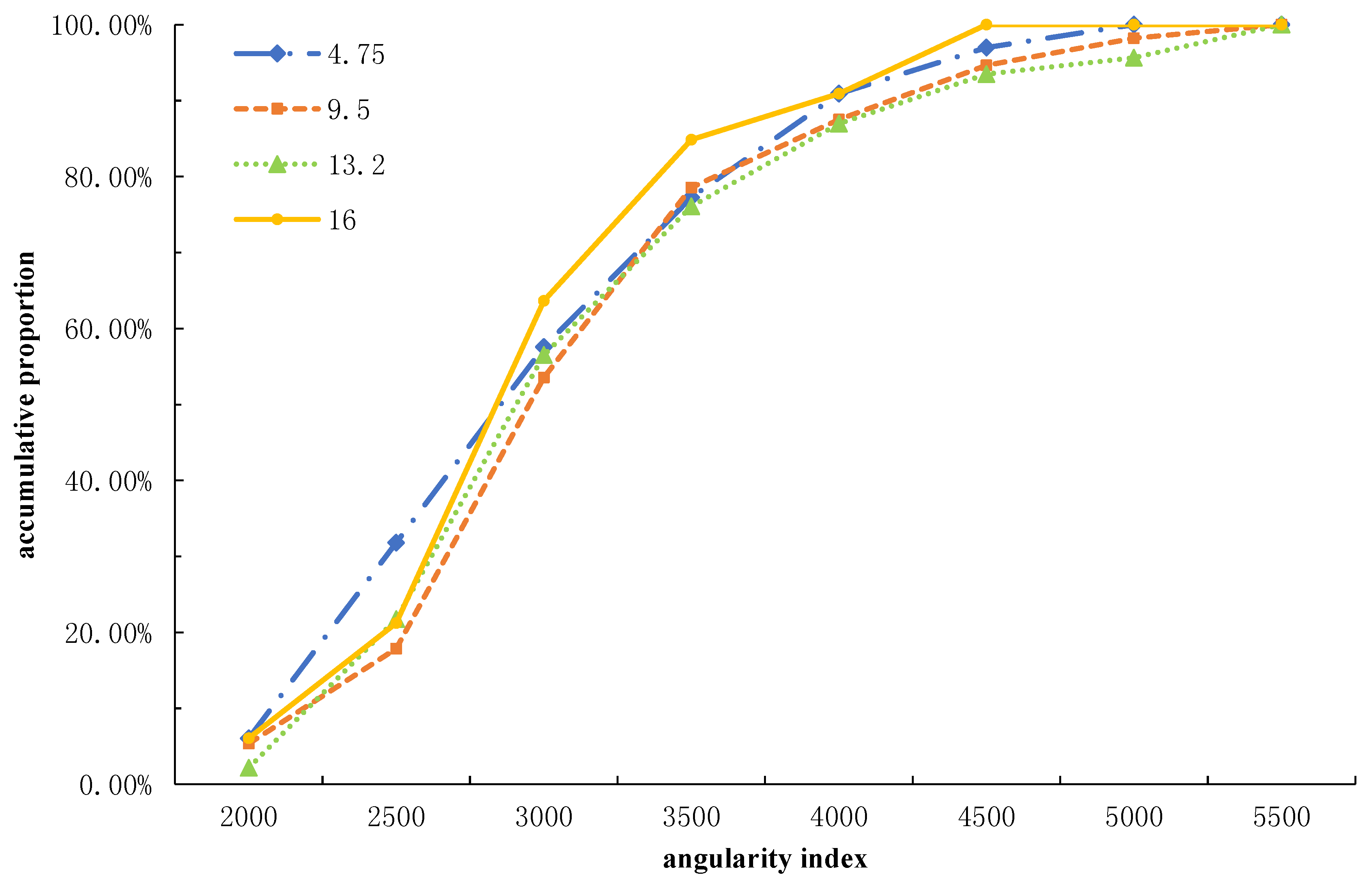
After the particle size was determined, . would be checked to develop the various angular shapes of the particles based on the angularity index distribution, as shown in Figure 7. For example, for the 4.75-mm particles, the process was conducted as following.
- ①If , only 4.75-mm particles with the angularity index ranging from 1500–2000 would be generated;
- ②If , only 4.75-mm particles with the angularity index ranging from 2000–2500 would be generated;
- ③If , only 4.75-mm particles with the angularity index ranging from 2500–3000 would be generated;
- ④If , only 4.75-mm particles with the angularity index ranging from 3000–3500 would be generated;
- ⑤If , only 4.75-mm particles with the angularity index ranging from 3500–4000 would be generated;
- ⑥If , only 4.75-mm particles with the angularity index ranging from 4000–4500 would be generated;
Enough particles were scanned and rebuilt within PFC2D. Thus, when was checked and the angularity index range was determined, corresponding virtual particles with the required shape would be generated by the user-defined routine. By the control of and , the virtual specimen could be developed with random particles obviously.
4.3. Example of Generating a Virtual Specimen
D, h and K were set as 15 cm, 12 cm and 35% during the modeling process, which was in accordance with the laboratory tests. The calculated mapping area is an important parameter to control the particles’ generation. The virtual aggregates were generated three times when forming the numerical models, as shown in Figure 8. When simulated, only one third of the mapping area was taken to determine the required number of different grades of aggregates. The virtual particles were generated one by one above the container and then fell down under gravity. Each time the generation completed, the specimen would be compacted by a virtual wall developed within PFC2D. The compacted wall would move downwards until reaching the designed height so as to achieving the required void content. By three cyclical steps, the virtual specimen could be developed as shown in Figure 8.
The generation routine of each grade of aggregate would be carried out until the total area of the generated particles exceeded the requirements. After the modeling completed, the total area of generated particles with different sizes was measured within PFC2D, as shown in Table 4. As shown, the generated virtual specimen was in good accordance with the actual gradations. The error was 5.51%, 3.86% and 3.70% for the 13.2-, 9.5- and 4.75-mm coarse aggregates, respectively. The error was attributed to the last generated particles, which exceeded the required mapping area, and it can be ignored. Thus, it is concluded that the proposed algorithm can well characterize the composition features of the aggregate specimen with precise particle shape reconstitutions and consistent gradation modeling.
5. Performance Prediction of the Rebuilt Models
5.1. Experiments
The penetration test using a Universal Testing Machine (UTM: Fuel Instruments & Engineers Pvt. Ltd. Maharashtra, India) was designed to measure the penetration force with the rod depth based on the Chinese test standard (JTG E40-2007: T0134-1993) [36]. A cylinder container with a diameter of 150 mm and a height of 120 mm was adopted during the tests. Then, three specimens with only the particles of 4.5, 9.5 and 13.2 mm were developed and were compacted based on the Chinese test standard (JTG E40-2007: T0131-2007) [36]. When conducting the penetration test, a rod would penetrate into the specimens slowly at a speed of 1.27 mm/min. Then, the force-displacement curves were recorded by the detectors.
To help the reconstitution of the virtual specimens, several data should also be measured before or after the laboratory tests, including the particle density, the density and the void contents of the compacted specimens, as shown in Table 5. The particle density is an input variable in DEM simulations to model the entities’ total mass, while the density and void contents of the compacted specimens were utilized to calculate the mapping area of coarse aggregates according to the proposed algorithm. The measurements for the particle density, the density and void contents of the compacted specimens were carried out based on the Chinese test standard, respectively (JTG E42-2005: T0308-2005, T0309-2005) [37].
5.2. Simulations for Performance Prediction
Prior to simulations, several micromechanical models were adopted to characterize the contact behavior between coarse aggregates within PFC2D; including the contact-stiffness model and sliding model [38], as the following equation shows.
Contact-stiffness model:
where is the normal force at the i-th contact point; is the shear contact force increment at the i-th contact point; is the normal stiffness at the contact; is the shear stiffness at the contact; is the overlap of the two contact entities along the normal direction; is the overlap of the two contact entities along the shear direction.
Sliding model:
where is the maximum allowable shear contact force; is the normal contact force between two entities; μ is the friction coefficient in PFC2D.
As shown in Equations (13) and (14), the contact force between two entities (balls) in the normal/shear direction was determined by the contact normal/shear stiffness and their overlap in corresponding directions. As for the normal contact force, the formula is always effective in the simulation, such that the intensity of depends on the value of and directly. However, the shear contact force was controlled and calculated based on two different modes for different periods. At the beginning, the shear contact force increment depends on and , when the adjacent entities contact each other. As the accumulative shear force reaches the limiting condition, as shown in Equation (14), the calculation process is converted immediately, in which the intensity of the shear contact force (not the shear force increment) is determined by the friction coefficient and absolute value of the normal contact force currently. As shown, it is significantly important to determine the values of and for modeling the micro-contact process in the simulation. According to the PFC2D manual, these two key micro-parameters are calculated by the input value of the balls’ normal stiffness and shear stiffness , respectively. The appropriate values of and can be obtained through a calibration process during the simulation based on the laboratory results. When calibrating the micro-parameters, the size influences should be taken into consideration. This means that the micro-parameters differed from each other for different sizes of particles and should be determined based on the size, respectively.
Thus, the simulations were conducted in two steps. In the first step, the virtual penetration tests of three different compositions were simulated. The three virtual specimens were developed by the proposed algorithm with 4.75-, 9.5- and 13.2-mm particles only, respectively. Then, the calibrated process for the best micro-parameters was done as follows: (1) conduct the laboratory penetration test to get the actual force-displacement curve of the three specimens; (2) conduct the simulations to get the virtual force-displacement curve of the three specimens; (3) obtain the best group of micro-parameters by adjusting their values continuously until the force-displacement curve of the simulation is close to the actual result. By the former process, the calibrated parameters can be obtained as shown in Table 6.
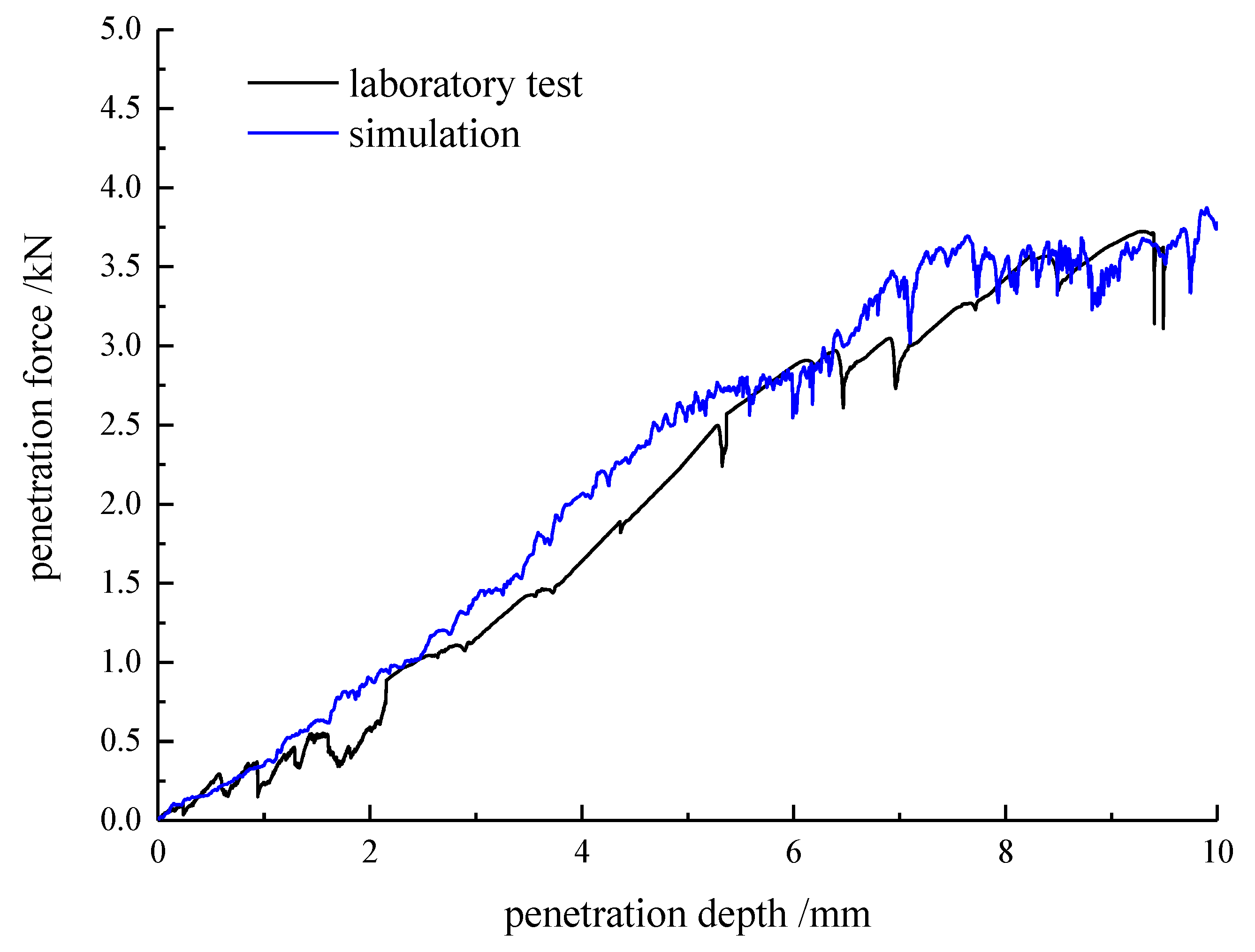
In the second step, the performance prediction of the SMA13 aggregate skeleton was done by the virtual penetration test. Moreover, the validation of the proposed algorithm was verified by comparing the prediction results with the actual ones. The virtual aggregate skeleton of SMA13 was formed and tested with the rod moving downward at a speed of 1.27 mm/min. Each particle was assigned the best micro-parameters based on Table 6. The prediction results and the actual force-displacement curve are illustrated in Figure 9. Since assumptions were made that there was no breakage or fraction during modeling, only 10-mm penetration depths were simulated. When the depth was less than 10 mm, there was no obvious breakage of the particles in laboratory tests, which can be used for nonlinear mechanical behavior predictions. It is obviously seen that the developed virtual models indeed have a good agreement with the results of the laboratory tests. The proposed algorithm was validated, which can not only model the aggregate shape precisely, but also characterize its mechanical performance well with the calibrated micro-parameters.
6. Conclusions
This paper proposed an algorithm for the reconstitution of the virtual aggregates and specimens based on the DEM methods. By the triangle area’s division, the irregular shape of the coarse aggregates can be formed well, and their mechanical performance was validated through the designed simulations. The main conclusions drawn from the study are as follows:
- (1)
- The scanning images from the AIMS are significant and guarantee the precise modelling of the coarse aggregates. The realistic shapes of the aggregates were captured and quantified through the inner software within AIMS. By generating the balls in the shape contours and then filling the inner area with balls by the proposed triangle-dividing algorithm, the virtual particles could be rebuilt, which had the same shapes as the realistic ones;
- (2)
- The mapping area was calculated to convert the three-dimensional volume to a two-dimensional area. Two random variables drawn from the uniform distribution (0, 1) were utilized to control the particles’ generation randomly. It was shown that the developed virtual specimen had a good accordance with the required gradations with minor errors of 5.51%, 3.86% and 3.70% for the 13.2-, 9.5- and 4.75-mm coarse aggregates, respectively. Thus, not only the particle shape, but also the heterogeneous composition within the structures could be modelled accurately;
- (3)
- Based on the calibrated micro-parameters, the mechanical performance of the aggregate skeleton could be well predicted through the proposed algorithm, which was verified by the virtual penetration test of the coarse aggregate skeleton with the SMA-13 gradation.
Author Contributions
D.W. and T.M. conceived and designed the experiments; X.D. performed the numerical experiments; W.Z. performed the laboratory experiments; D.Z. contributed analysis tools; D.W. and X.D. wrote the paper.
Acknowledgments
The study was financially supported by the Science Foundations of Nanjing Institute of Technology, China (YKJ201423), the National Natural Science Foundation of China (No. 51378006) and the Natural Science Foundation of Jiangsu Province, China (BK20161421).
Conflicts of Interest
The authors declare no conflict of interest.
References
- Pan, T.; Tutumluer, E.; Carpenter, S.H. Effect of Coarse Aggregate Morphology on Permanent Deformation Behavior of Hot Mix Asphalt. J. Transp. Eng. 2015, 132, 580–589. [Google Scholar] [CrossRef]
- Ramli, I. Effect of Fine Aggregate Angularity on Rutting Resistance of Asphalt Concrete AC10; Universiti Teknologi Malaysia: Iskandar Puteri, Malaysia, 2013. [Google Scholar]
- Shah, S.M.R.; Abdullah, M.E. Effect of Aggregate Shape on Skid Resistance of Compacted Hot Mix Asphalt (HMA). In Proceedings of the 2010 the 2nd International Conference on Computer and Network Technology (ICCNT), Bangkok, Thailand, 23–25 April 2010; IEEE: Piscataway, NJ, USA, 2010; pp. 421–425. [Google Scholar]
- Campen, W.H.; Smith, J.R. A study of the role of angular aggregates in the development of stability in bituminous mixtures. Proc. AAPT 1948, 17, 114–143. [Google Scholar]
- Kandhal, P.S.; Parker, F. Aggregate Tests Related to Asphalt Concrete Performance in Pavements; National Cooperative Highway Research Program Report 405; Transportation Research Board: Washington, DC, USA, 1998. [Google Scholar]
- Cheung, L.W.; Dawson, A. Effects of particle and mix characteristics on performance of some granular materials. Transp. Res. Rec. J. Transp. Res. Board 2002, 1787, 90–98. [Google Scholar] [CrossRef]
- Hossain, M.; Parker, F., Jr.; Kandhal, P. Tests for evaluating fine aggregate particle shape, angularity, and surface texture. Transp. Res. Rec. J. Transp. Res. Board 1999, 1673, 64–72. [Google Scholar] [CrossRef]
- Hossain, M.S.; Parker, F.; Kandhal, P.S. Comparison and evaluation of tests for coarse aggregate particle shape, angularity, and surface texture. J. Test. Eval. 2000, 28, 77–87. [Google Scholar]
- Cundall, P.A. Ball-A Program to Model Granular Media Using the Distinct Element Method; Technical Note; Advanced Technology Group, Dames & Moore: London, UK, 1978. [Google Scholar]
- Ma, T.; Wang, H.; Zhang, D.; Zhang, Y. Heterogeneity effect of mechanical property on creep behavior of asphalt mixture based on micromechanical modeling and virtual creep test. Mech. Mater. 2017, 104, 49–59. [Google Scholar] [CrossRef]
- Mishra, B.K.; Rajamani, R.K. The discrete element method for the simulation of ball mills. Appl. Math. Model. 1992, 16, 598–604. [Google Scholar] [CrossRef]
- Su, O.; Akcin, N.A. Numerical simulation of rock cutting using the discrete element method. Int. J. Rock Mech. Min. Sci. 2011, 48, 434–442. [Google Scholar] [CrossRef]
- Lu, M.; McDowell, G.R. The importance of modelling ballast particle shape in the discrete element method. Granul. Matter 2007, 9, 69. [Google Scholar] [CrossRef]
- Das, N.; Thomas, S.; Kopmann, J.; Donovan, C.; Hurt, C.; Daouadji, A.; Ashmawy, A.K.; Sukumaran, B. Modeling Granular Particle Shape Using Discrete Element Method. Mon. Not. R. Astron. Soc. 2008, 420, 3368–3380. [Google Scholar]
- Coetzee, C.J. Calibration of the discrete element method and the effect of particle shape. Powder Technol. 2016, 297, 50–70. [Google Scholar] [CrossRef]
- Zhang, D.; Huang, X.; Zhao, Y. Algorithms for generating three-dimensional aggregates and asphalt mixture samples by the discrete-element method. J. Comput. Civ. Eng. 2012, 27, 111–117. [Google Scholar] [CrossRef]
- Stahl, M.; Konietzky, H. Discrete element simulation of ballast and gravel under special consideration of grain-shape, grain-size and relative density. Granul. Matter 2011, 13, 417–428. [Google Scholar] [CrossRef]
- Huang, H. Discrete Element Modeling of Railroad Ballast Using Imaging Based Aggregate Morphology Characterization. Ph.D. Thesis, University of Illinois at Urbana-Champaign, Urbana, IL, USA, 2010. [Google Scholar]
- Liu, Y.; You, Z. Visualization and simulation of asphalt concrete with randomly generated three-dimensional models. J. Comput. Civ. Eng. 2009, 23, 340–347. [Google Scholar] [CrossRef]
- Liu, Y.; You, Z. Accelerated Discrete-Element Modeling of Asphalt-Based Materials with the Frequency-Temperature Superposition Principle. J. Eng. Mech. 2011, 137, 355–365. [Google Scholar] [CrossRef]
- Tutumluer, E.; Qian, Y.; Hashash, Y.M.A.; Davis, D. Field validated discrete element model for railroad ballast. In Proceedings of the Annual Conference of the American Railway Engineering and Maintenance-of-Way Association, Minneapolis, MN, USA, 18–21 September 2011; pp. 18–21. [Google Scholar]
- Dondi, G.; Simone, A.; Vignali, V.; Manganelli, G. Numerical and experimental study of granular mixes for asphalts. Powder Technol. 2012, 232, 31–40. [Google Scholar] [CrossRef]
- Dondi, G.; Simone, A.; Vignali, V.; Manganelli, G. Discrete Element Modelling of Influences of Grain Shape and Angularity on Performance of Granular Mixes for Asphalts. Procedia Soc. Behav. Sci. 2012, 53, 399–409. [Google Scholar] [CrossRef]
- Vignali, V. Discrete particle element analysis of aggregate interaction in granular mixes for asphalt: Combined DEM and experimental study. In 7th Rilem International Conference on Cracking in Pavements; Springer: Berlin, Germany, 2012; pp. 389–398. [Google Scholar]
- Fu, Y.; Wang, L.; Tumay, M.T.; Li, Q. Quantification and simulation of particle kinematics and local strains in granular materials using X-ray tomography imaging and discrete-element method. J. Eng. Mech. 2008, 134, 143–154. [Google Scholar] [CrossRef]
- Moreno-Atanasio, R.; Williams, R.A.; Jia, X. Combining X-ray microtomography with computer simulation for analysis of granular and porous materials. Particuology 2010, 8, 81–99. [Google Scholar] [CrossRef]
- Wang, L.; Park, J.Y.; Fu, Y. Representation of real particles for DEM simulation using X-ray tomography. Constr. Build. Mater. 2007, 21, 338–346. [Google Scholar] [CrossRef]
- Hall, S.A.; Bornert, M.; Desrues, J.; Pannier, Y.; Lenoir, N.; Viggiani, G.; Bésuelle, P. Discrete and continuum analysis of localised deformation in sand using X-ray μCT and volumetric digital image correlation. Géotechnique 2010, 60, 315–322. [Google Scholar] [CrossRef]
- Alshibli, K.A.; Reed, A.H. Comparison of X-Ray CT and Discrete Element Method in the Evaluation of Tunnel Face Failure. In Advances in Computed Tomography for Geomaterials: GeoX 2010; John Wiley & Sons Inc.: Hoboken, NJ, USA, 2013; pp. 397–405. [Google Scholar]
- Liu, Y.; Zhou, X.; You, Z.; Yao, S.; Gong, F.; Wang, H. Discrete element modeling of realistic particle shapes in stone-based mixtures through MATLAB-based imaging process. Constr. Build. Mater. 2017, 143, 169–178. [Google Scholar] [CrossRef]
- Liu, Y.; You, Z.; Zhao, Y. Three-dimensional discrete element modeling of asphalt concrete: Size effects of elements. Constr. Build. Mater. 2012, 37, 775–782. [Google Scholar] [CrossRef]
- Gates, L.L. Experimental Evaluation of New Generation Aggregate Image Measurement System. Ann. Emerg. Med. 2010, 33, 611. [Google Scholar]
- Araujo, V.M.C.; Bessa, I.S.; Branco, V.T.F.C. Measuring skid resistance of hot mix asphalt using the aggregate image measurement system (AIMS). Constr. Build. Mater. 2015, 98, 476–481. [Google Scholar] [CrossRef]
- Rezaei, A.; Hoyt, D.; Martin, A.E. Simple Laboratory Method for Measuring Pavement Macrotexture Pavement Cores and Aggregate Image Measurement System. Transp. Res. Rec. J. Transp. Res. Board 2011, 2227, 146–152. [Google Scholar] [CrossRef]
- Luce, A.D. Analysis of Aggregate Imaging System (AIMS) Measurements and Their Relationship to Asphalt Pavement Skid Resistance; Texas A & M. University: College Station, TX, USA, 2009. [Google Scholar]
- Ministry of Transport of the People’s Republic of China. Test. Methods of Soils for Highway Engineering; JTG E40-2007; China Communications Press: Beijing, China, 2007.
- Ministry of Transport of the People’s Republic of China. Test. Methods of Aggregates for Highway Engineering; JTG E42-2005; China Communications Press: Beijing, China, 2005.
- Itasca Consulting Group. PFC 2D Version 4.0; Itasca Consulting Group: Minneapolis, MN, USA, 2004. [Google Scholar]
Figure 1.
Binary images of aggregate particles: (a) shape; (b) shape contour.

Figure 2.
Triangle area divisions for measurement.

Figure 3.
Algorithm for filling the triangle area with discrete balls: (a) ; (b) > .

Figure 4.
Conversions between local and global coordinate systems.
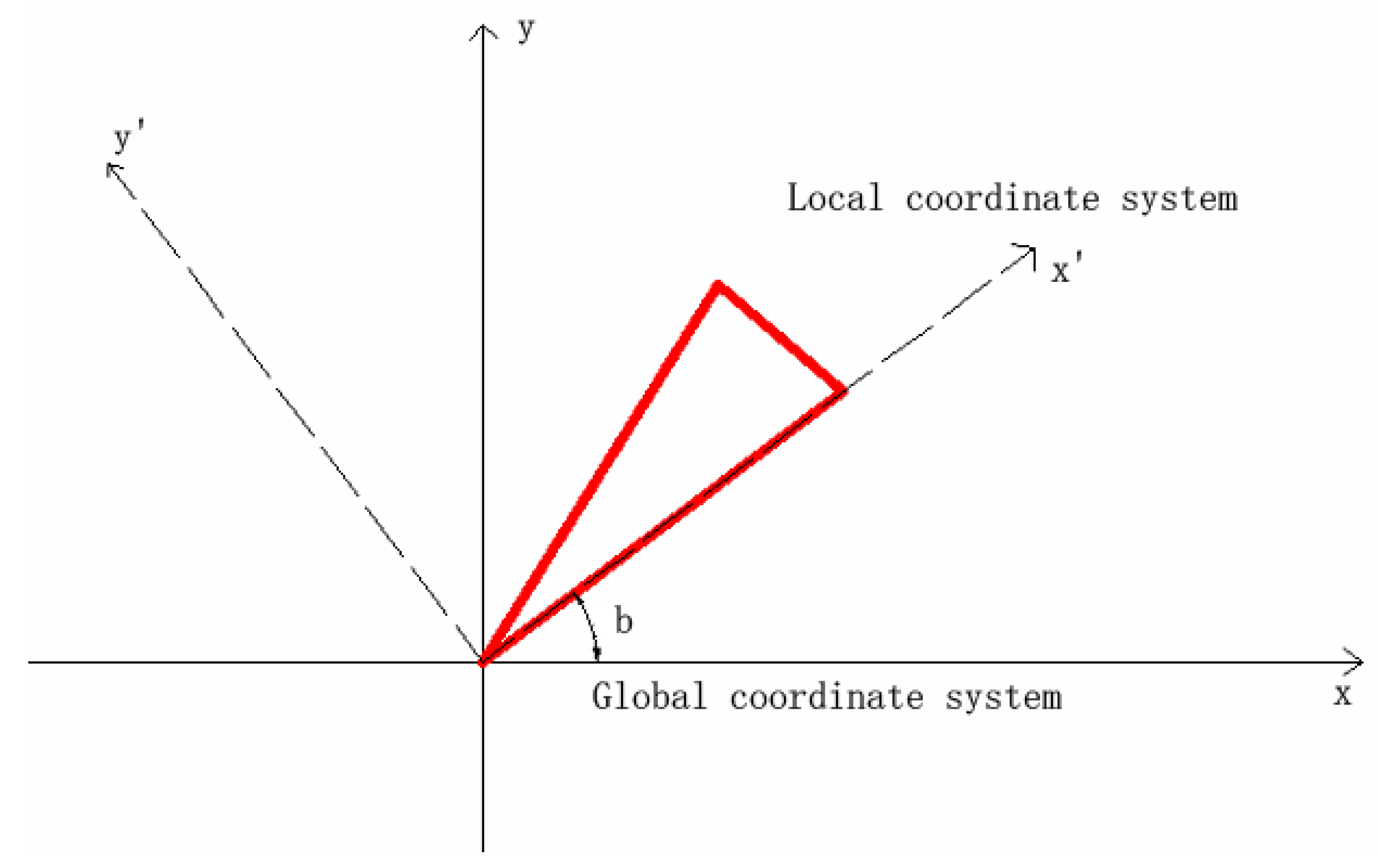
Figure 5.
Procedure of the virtual particles’ modeling.
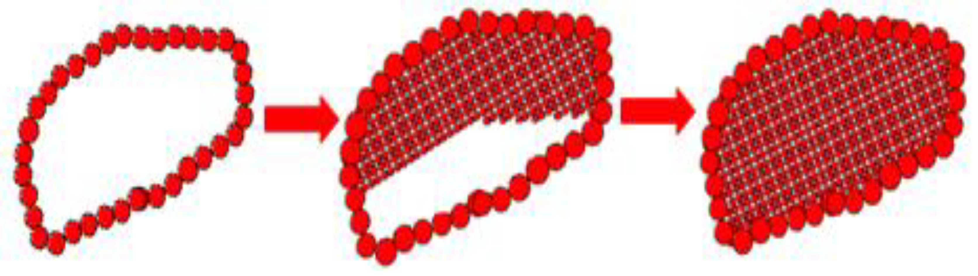
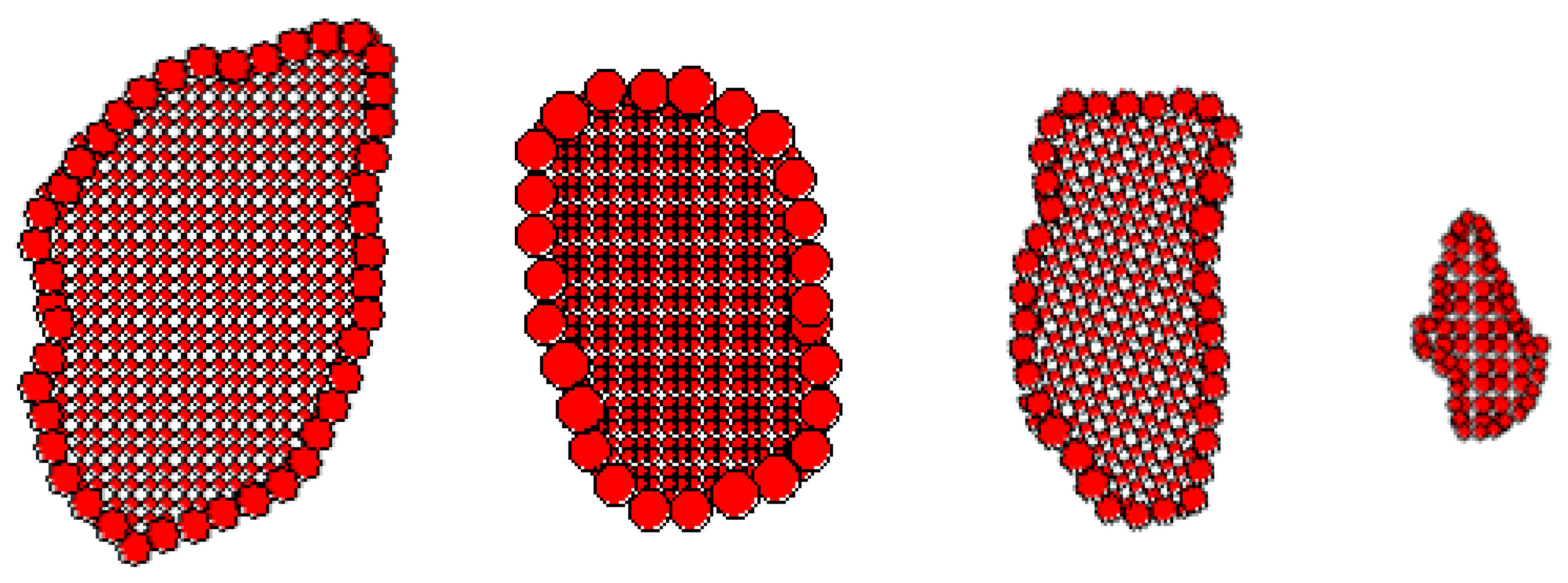
Figure 6.
Various virtual particles of different morphological characteristics.

Figure 7.
Angularity index distribution of different sizes of particles.

Figure 8.
Modeling procedure of the virtual specimens: (a) first step of generation; (b) second step of generation; (c) third step of generation.
Figure 8.
Modeling procedure of the virtual specimens: (a) first step of generation; (b) second step of generation; (c) third step of generation.
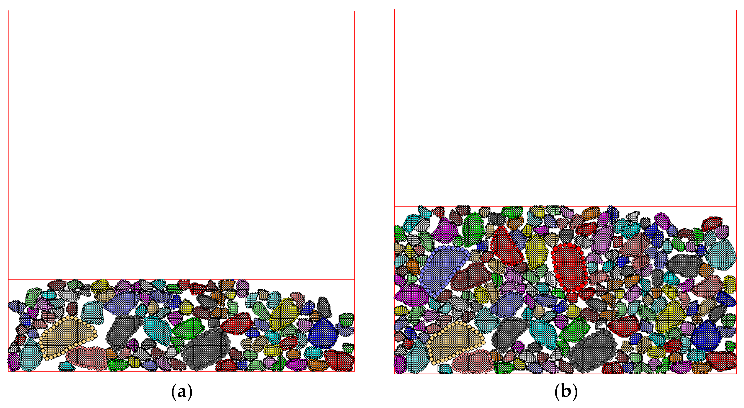

Figure 9.
Prediction results of SMA-13.


Table 1.
Summaries of the two-dimensional images.
| Sample | Angularity | Reduction Scale | Particle Area (m2) |
|---|---|---|---|
| 1 | 2864.41 | 4109.07 | 0.00033 |
| 2 | 3358.80 | 2882.90 | 0.00040 |
| 3 | 1803.25 | 1692.92 | 0.00045 |
| 4 | 2354.54 | 2015.89 | 0.00053 |
| 5 | 4329.94 | 2174.40 | 0.00038 |
| 6 | 3641.75 | 1925.21 | 0.00056 |
| 7 | 2192.07 | 3589.41 | 0.00036 |
| 8 | 3716.14 | 3527.46 | 0.00043 |
| 9 | 2040.78 | 4591.80 | 0.00028 |
Table 2.
Adjustments of the image coordinates.
| Sample | Adjustments of X-Coordinate | Adjustments of Y-Coordinate |
|---|---|---|
| 1 | −74.53354 | −100.6707 |
| 2 | −75.23496 | −103.149 |
| 3 | −76.80114 | −100.0369 |
| 4 | −74.9621 | −104.7988 |
| 5 | −75.26646 | −102.7743 |
| 6 | −72.68012 | −100.83 |
| 7 | −78.78299 | −98.05279 |
| 8 | −74.50542 | −101.9675 |
| 9 | −80.44268 | −105.0318 |
Table 3.
Gradation for SMA-13.
| Gradation | Passing Ratio (%) for Different Sieving Sizes (mm) | |||||||||
|---|---|---|---|---|---|---|---|---|---|---|
| 16 | 13.2 | 9.5 | 4.75 | 2.36 | 1.18 | 0.6 | 0.3 | 0.15 | 0.075 | |
| SMA-13 | 100 | 95 | 79.5 | 48.9 | 36.7 | 25.8 | 16.7 | 9.7 | 7.1 | 6.5 |
Table 4.
Summaries of the virtual modeling.
| Sieving size (mm) | 13.2 | 9.5 | 4.75 |
| Required mapping area () | 11.44 | 35.21 | 70.06 |
| Total area of generated particles () | 12.07 | 36.57 | 72.65 |
| Error (%) | 5.51 | 3.86 | 3.70 |
Table 5.
Materials for laboratory penetration tests.
| Sieving Size (mm) | Particle Density (g/cm3) | Density of Compacted Specimen (g/cm3) | Void Contents of Compacted Specimens (%) |
|---|---|---|---|
| 13.2 | 2.744 | 1.625 | 39.55 |
| 9.5 | 2.730 | 1.616 | 39.66 |
| 4.75 | 2.729 | 1.594 | 40.70 |
Table 6.
Calibrated micro-parameters for balls and walls within Particle Flow Code in Two Dimensions (PFC2D).
Table 6.
Calibrated micro-parameters for balls and walls within Particle Flow Code in Two Dimensions (PFC2D).
| Size/mm | μ | |||
|---|---|---|---|---|
| ball | 4.75 | 2.2e6 | 1.5e6 | 0.6 |
| 9.5 | 2.5e6 | 2.5e6 | 0.55 | |
| 13.2 | 1.2e6 | 1.2e6 | 0.5 | |
| wall | 1e10 | 1e10 | 0.6 | |
© 2018 by the authors. Licensee MDPI, Basel, Switzerland. This article is an open access article distributed under the terms and conditions of the Creative Commons Attribution (CC BY) license (http://creativecommons.org/licenses/by/4.0/).
Share and Cite
MDPI and ACS Style
Wang, D.; Ding, X.; Ma, T.; Zhang, W.; Zhang, D. Algorithm for Virtual Aggregates’ Reconstitution Based on Image Processing and Discrete-Element Modeling. Appl. Sci. 2018, 8, 738. https://doi.org/10.3390/app8050738
AMA Style
Wang D, Ding X, Ma T, Zhang W, Zhang D. Algorithm for Virtual Aggregates’ Reconstitution Based on Image Processing and Discrete-Element Modeling. Applied Sciences. 2018; 8(5):738. https://doi.org/10.3390/app8050738
Chicago/Turabian StyleWang, Danhua, Xunhao Ding, Tao Ma, Weiguang Zhang, and Deyu Zhang. 2018. "Algorithm for Virtual Aggregates’ Reconstitution Based on Image Processing and Discrete-Element Modeling" Applied Sciences 8, no. 5: 738. https://doi.org/10.3390/app8050738
Note that from the first issue of 2016, this journal uses article numbers instead of page numbers. See further details here.