Virtual Diagnostic Sensors Design for an Automated Guided Vehicle

Abstract

In recent years, Automated Guided Vehicles (AGVs) have been playing an increasingly important role in producing industry and infrastructure and will soon arrive to other areas of human life such as the transportation of goods and people. However, several challenges still aggravate the operation of AGVs, which limit the amount of implementation. One major challenge is the realization of reliable sensors that can capture the different aspects of the state of an AGV as well as its surroundings. One promising approach towards more reliable sensors is the supplementary application of virtual sensors, which are able to generate virtual measurements by using other sources of information such as actuator states and already existing sensors together with appropriate mathematical models. The focus of the research described in this paper is the design of virtual sensors determining forces and torques acting on an AGV. The proposed novel approach is using a quadratic boundedness approach, which makes it possible to include bounded disturbances acting on the AGV. One major advantage of the presented approach is that the use of complex tire models can be avoided. Information from acceleration and yaw rate sensors is processed in order to realize reliable virtual force and torque sensors. The resulting force and torque information can be used for several diagnostic purposes such as fault detection or fault prevention. The presented approach is explained and verified on the basis of an innovative design of an AGV. This innovative design addresses another major challenge for AGVs, which is the limited maneuvering possibilities of many AGV designs. The innovative design allows nearly unlimited maneuvering possibilities but requires reliable sensor data. The application of the approach in the AGV resulted in the insight that the generated estimates are consistent with the longitudinal forces and torques obtained by a proven reference model.

1. Introduction

Automated guided vehicles can be used in any scenario with prominent material flows. Applications of Automated Guided Vehicles (AGVs) exist in all fields of industry and trade. Typical examples are the use in assembly lines, warehouses, order picking systems and production plants [1]. The main motivation of the presented research is the still relatively low application rate of AGVs. In theory, AGVs dispose of several advantages compared to other kinds of logistics equipment. They are more flexible, modular and intelligent, use less field area and require little time and cost for initial installation [2]. However, until today, AGVs have not yet been applied in many potential applications [3]. Additionally, frequently, even if AGVs are already applied, their possible potential in terms of flexibility and efficiency is not yet exploited because they are only used for rather mundane tasks such as good loading and unloading and only fixed guiding technology such as magnetic guidance or optical guidance are used [2]. One main problem can be the hardware design [2]. AGVs with conventional steering systems such as classical Ackermann steering exhibit limited maneuvering capability and can thus not use the movement areas efficiently. Another main problem is the high cost of sensors in AGVs and the fact that sensor data filtering, sensor data plausibility assessment and sensor fusion are no trivial tasks. In real AGV operation, some parameters such as slip, exact wheel diameter and mass are changed during the operation caused by uneven load distribution or manufacturing imperfection and loading of goods [4]. These conditions aggravate the gathering of reliable sensor data. Further problems can arise from a less than sufficient flexibility, availability and reliability of current AGV designs. The main objective of the presented research is to develop approaches for optimized virtual sensor design and, through this, to more efficient, flexible and reliable AGVs. The presented research combines two main approaches to address these causes: the innovative AGV design, which is described in this paper, allows unlimited maneuvering capabilities and the virtual diagnostic sensor design enhances reliable sensor information without additional expenditures.

2. Research Thesis and Structure

In recent years, a considerable amount of research is centered on Fault-Tolerant Control (FTC) systems, which can be envisioned to maintain control objectives even if a fault occurs. The application of such system is frequently hindered by a lack of reliable sensors and the high cost of sensors [5,6,7]. Therefore, virtual sensors are applied, which make use of mathematical models of the process and other available measurements to estimate the unmeasured variables [8,9]. Many approaches have been reported to design virtual diagnostic sensors: for instance, observer-based [10,11], Kalman filter-based [12,13] and parameter identification-based [14] approaches.

At the center of the research is an innovative approach to virtual sensor design of longitudinal forces as well as torques acting onto an AGV using a Quadratic Boundedness (QB) approach [15]. This approach allows for including bounded disturbances acting on the AGV and avoids unnecessary state estimation because the state is fully available via measurements. One main advantage of the innovative approach is that the application of sophisticated tire models is not necessary. Frequently, the application of these kinds of models limits the performance of the approaches presented in the literature [16,17]. Another main advantage of the proposed approach is that the design procedure is expressed in the form of Linear Matrix inequalities (LMIs), which can be solved using widely available computational packages.

Consequently, the central research thesis can be stated as follows: is it possible to design reliable virtual sensors for longitudinal forces and torques of automated guided vehicles based on a quadratic boundedness approach?

An innovative design of an AGV, which allows unlimited maneuvering capabilities but requires reliable sensor information is used both for the sake of explanation and validation of the approach.

It should also be pointed out that such kind of problems can be potentially tackled with the so-called direct virtual sensors, which instead of exploiting the identified system dynamics are based strictly on the existing data [18,19,20,21,22]. This is, however, beyond the scope of the developments presented in this paper, which are strictly based on an analytical model of the AGV.

The paper is organized as follows. Section 3 introduces essential preliminaries, which are necessary to undertake the problem being investigated. Section 4 describes the AGV, which will be used in this work for the sake of explanation and validation. Section 5 presents the mathematical foundation. Section 6 proposes a strategy for the design of the virtual diagnostic sensor. Section 7 presents the results of the application of the proposed strategy to the AGV. Section 8 shows experimental results, which clearly exhibit the performance of the proposed approach. Finally, the last section concludes the paper.

3. Description of Discrete Time Systems

Let us consider the following time-varying discrete-time system

$${\mathit{x}}_{k+1}={\mathit{A}}_k{\mathit{x}}_k+{\mathit{B}}_k{\mathit{u}}_k+{\mathit{E}}_k{\mathit{d}}_k+\mathit{W}{\mathit{w}}_k,$$

(1)

where ${\mathit{x}}_k\in \mathbb{X}\subset {\mathbb{R}}^n$ is the state vector, ${\mathit{u}}_k\in \mathbb{U}\subset {\mathbb{R}}^r$ stands for the input, ${\mathit{d}}_k\in \mathbb{D}\subset {\mathbb{R}}^{n_d}$ is an unknown input, and ${\mathit{w}}_k\in \mathcal{E}\subset {\mathbb{R}}^{n_w}$ is an exogenous disturbance vector with

$$\begin{array}{c}\hfill {\mathit{w}}_k\in \mathcal{E},\mathcal{E}=\{\mathit{w}:{\mathit{w}}^T{\mathit{Q}}_{\mathit{w}}\mathit{w}\le 1\},{\mathit{Q}}_{\mathit{w}}\succ 0.\end{array}$$

(2)

Let $V_k={\mathit{x}}_k^T\mathit{P}{\mathit{x}}_k$ denote a Lyaponov candidate function. For an unforced ${\mathit{u}}_k=\mathbf{0}$ and unknown input-free ${\mathit{d}}_k=\mathbf{0}$ system (1), the following definitions are recalled [15,23]:

Definition 1.

The system (1) is strictly quadratically bounded for all allowable ${\mathit{w}}_k\in \mathcal{E}$, $k\ge 0$, if

$$V_k>1\Rightarrow V_{k+1}-V_k<0,$$

(3)

for any ${\mathit{w}}_k\in \mathcal{E}$.

Definition 2.

A set ${\mathcal{E}}_{\mathit{x}}$ is a robust invariant set for the system (1) for all allowable ${\mathit{w}}_k\in \mathcal{E}$ if

$${\mathit{x}}_k\in {\mathcal{E}}_{\mathit{x}}\Rightarrow {\mathit{x}}_{k+1}\in {\mathcal{E}}_{\mathit{x}},$$

(4)

for any ${\mathit{w}}_k\in \mathcal{E}$.

It should be pointed out that the strict quadratic boundedness enables decreasing the value of Lyapunov function $V_k$, i.e., it means that $V_{k+1}<V_k$ for any ${\mathit{w}}_k\in \mathcal{E}$ when $V_k>1$. If Equation (1) is quadratically bounded and there exists at least one vector $\mathit{W}{\mathit{w}}_k\ne 0$, then such quadratic boundedness is always strict [15]. Moreover, the notation of the quadratic boundedness can be expressed using the theory of invariant sets [15]. The set ${\mathcal{E}}_{\mathit{x}}=\{\mathit{x}:{\mathit{x}}_{}^T\mathit{P}\mathit{x}\le 1\}$ is an invariant set for any ${\mathit{w}}_k\in \mathcal{E}$ if ${\mathit{x}}_k\in {\mathcal{E}}_{\mathit{x}}$ implies ${\mathit{x}}_{k+1}\in {\mathcal{E}}_{\mathit{x}}$. Thus, if $V_k>1,$ then ${\mathit{x}}_k$ is outside an invariant set, and, hence, by Definition 1 $V_{k+1}<V_k$. This means that $V_k$ decreases until ${\mathit{x}}_k$ is outside ${\mathcal{E}}_{\mathit{x}}$.

4. Design and Realization of an Automated Guided Vehicle

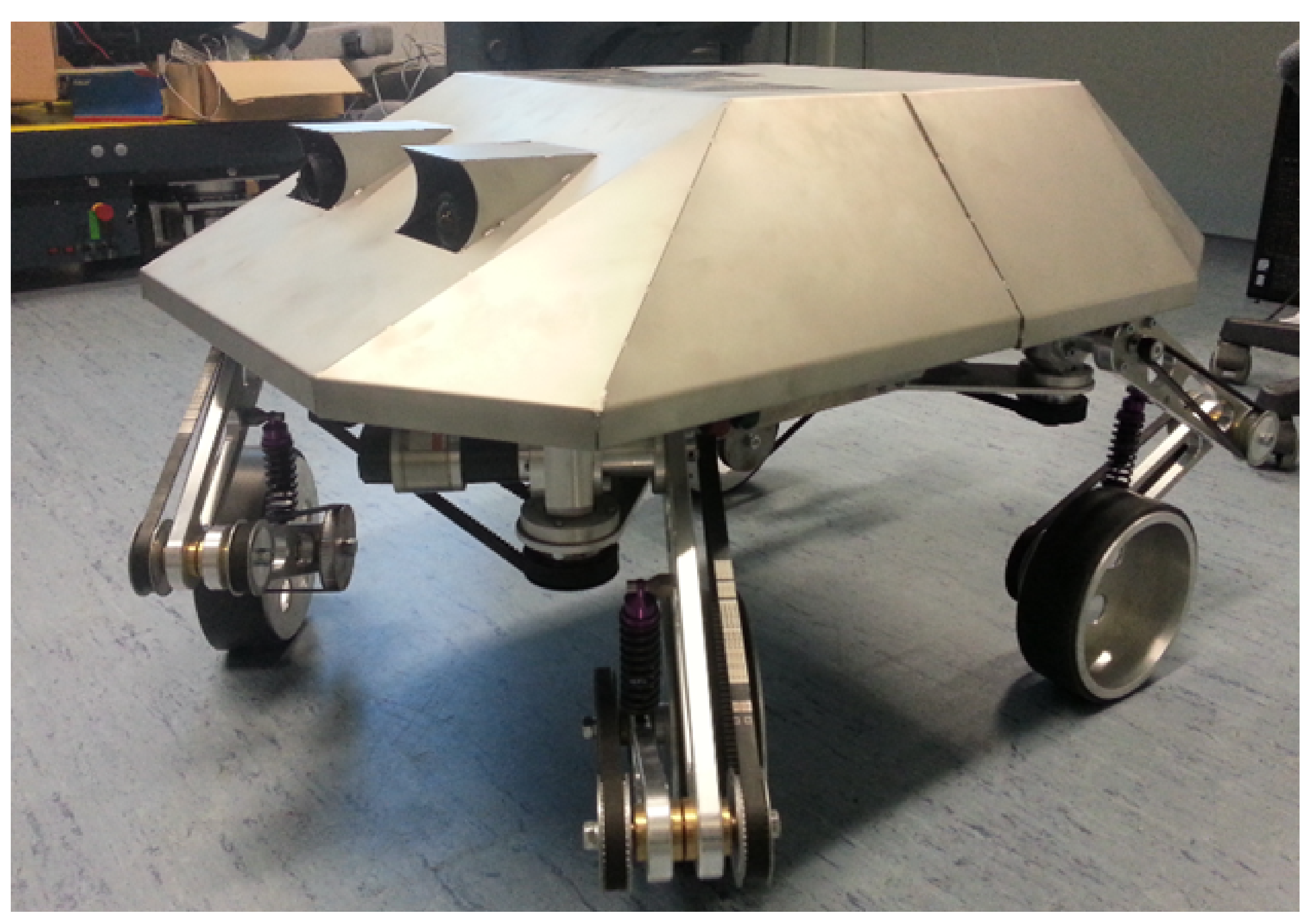
The main objective of the innovative AGV, which was developed at the University of Applied Sciences Ravensburg-Weingarten, was the realization of nearly unlimited maneuvering possibilities with a rather simple mechanical design (Figure 1).

In earlier work, a production platform with a patented steering principle was developed [24]. This production platform exhibited very good maneuvering possibilities [25], but required eight dedicated drive motors and was restricted to flat floors. The innovative design allows driving in uneven environments and only requires four drive motors. The AGV’s main frame consists of four sprung arms that each dispose of one drive motor. The arms can freely rotate, but the front arms and the back arms are connected by belts. Each drive motor disposes of an angle encoder. This allows for determining the angle, the angular velocity and the angular acceleration of each wheel. Another set of two angular encoders measures the steering angle of the front wheels and the back wheels, respectively. The use of four individual motor controllers (electronic position control EPOS—communicating via the CANopen protocol) enables independent use of each drive motor. The ability to use four independent motors leads to a steering system that is already registered as a patent and is based on the concept to use the torque differences between wheels to steer the axles of a vehicle. The AGV can drive directly in any direction without time- and space-consuming turning maneuvers and is able to turn around its own center. Especially in narrow spaces that are common in production settings, this characteristic is very desirable. Still, the mechanical construction is rather simple, because no dedicated steering motors are necessary. This leads to a high robustness. Apart from the six angular sensors mentioned above, the robot is equipped with global acceleration, velocity and yaw rate sensors, whose measurements are available via the Bluetooth protocol. Figure 2 shows the main parameters of the steering system of the AGV with all the considered forces and the parameters are additionally listed in

Table 1. Automated Guided Vehicles (AGVs) parameters.

Variable	Unit	Value
m	kg	50
$L_f$	m	0.25
$L_r$	m	0.25
$I_z$	$\mathrm{kg}/{\mathrm{m}}^2$	89.18
$C_r$	$\mathrm{kg}{/}^{\circ }$	1.86
$C_f$	$\mathrm{kg}{/}^{\circ }$	1.86
$L_a$	m	0.16
$R_e$	m	0.09
$I_{xw}$	$\mathrm{kg}/{\mathrm{m}}^3$	0.00209089

.

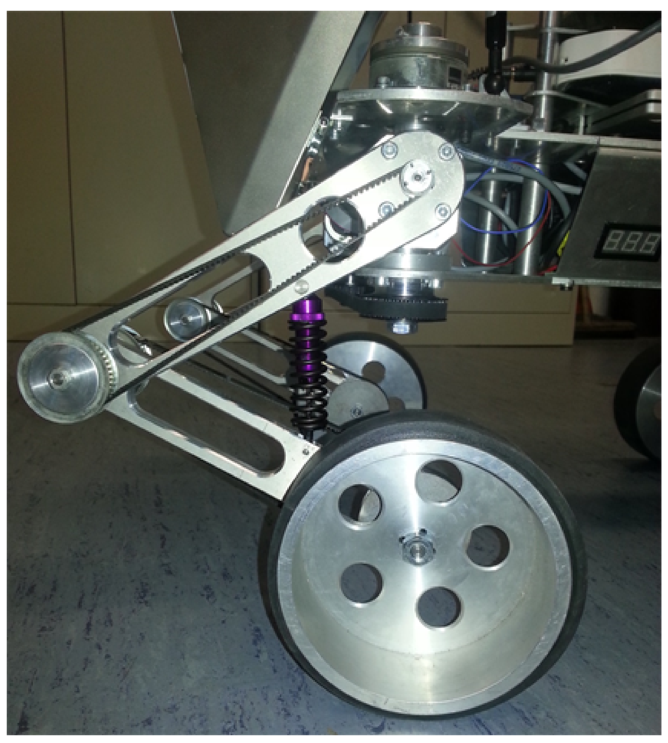
Each arm that holds a drive wheel disposes of a spring suspension intended to absorb impacts from uneven terrain and to balance possible different heights of the terrain (Figure 3).

For controlling the AGV different modes can be chosen: manual driving and an autonomous driving mode. A central control unit (PC ALIX) determines the required steering angles for the front and the back wheels and sends (different) angular velocity commands to the four drive motors in order to achieve the desired steering angle, the desired driving direction, the desired instantaneous center of rotation ICR (which is often infinitely far away) and the desired vehicle speed.

5. Mathematical Model of the Automated Guided Vehicle

Before proceeding with the development, let us provide the names of the crucial variables shaping the AGV dynamics, which are given in

Table 2. Notation.

$\mathit{COG}$	Center of Gravity
$i=front,rear$	axle location
$j=left,right$	wheel location
$L_f$	distance between front axle and COG
$L_r$	distance between rear axle and COG
$L_a$	rear/front half gauge
r	yaw rate
$v_x$	longitudinal velocity
$a_x$	longitudinal acceleration
$a_y$	lateral acceleration
m	mass
${\delta }_f$	steering angle of the front wheels
${\delta }_r$	steering angle of the rear wheels
$F_x$	sum of forces causing longitudinal motion
$F_y$	sum of forces causing lateral motion
$F_{x,ij}$	longitudinal force on $i,j$ wheel
$F_{y,f}$	total lateral force on the front wheels
$F_{y,r}$	total lateral force on the rear wheels
${\omega }_{i,j}$	angular velocity of $i,j$ wheel
T	total torque acting on all wheels
$p_{i,j}$	torque distribution coefficient
$I_{xw}$	wheel moment of inertia
$I_z$	robot moment of inertia around z-axis
$R_e$	wheel effective radius
$C_f$	front wheel cornering stiffness
$C_r$	rear wheel cornering stiffness

.

From Figure 2, it can be derived that the force causing longitudinal motion is given by

$$\begin{array}{c}\hfill \begin{array}{cc}\hfill F_x& =cos\left({\delta }_f\right)(F_{x,fl}+F_{x,fr})+cos\left({\delta }_r\right)(F_{x,rl}+F_{x,rr})+\hfill \\ & -sin\left({\delta }_f\right)F_{y,f}-sin\left({\delta }_r\right)F_{y,r}.\hfill \end{array}\end{array}$$

(5)

Analogously, the lateral forces can be analyzed:

$$\begin{array}{cc}\hfill F_y& =sin\left({\delta }_f\right)(F_{x,fl}+F_{x,fr})+sin\left({\delta }_r\right)(F_{x,rl}+F_{x,rr})+\hfill \\ & +cos\left({\delta }_f\right)F_{y,f}+cos\left({\delta }_r\right)F_{y,r},\hfill \end{array}$$

(6)

where the longitudinal wheel forces obey:

$$\begin{array}{cc}\hfill I_{xw}{\dot{\omega }}_{fl}& =p_{f,l}T-F_{x,fl}{R}_e,\hfill \end{array}$$

(7)

$$\begin{array}{cc}\hfill I_{xw}{\dot{\omega }}_{fr}& =p_{f,r}T-F_{x,fr}{R}_e,\hfill \end{array}$$

(8)

$$\begin{array}{cc}\hfill I_{xw}{\dot{\omega }}_{rl}& =p_{r,l}T-F_{x,rl}{R}_e,\hfill \end{array}$$

(9)

$$\begin{array}{cc}\hfill I_{xw}{\dot{\omega }}_{rr}& =p_{r,r}T-F_{x,rr}{R}_e,\hfill \end{array}$$

(10)

with the torque distribution coefficients $p_{i,j}\ge 0$ satisfying:

$$\begin{array}{c}\hfill p_{f,l}+p_{f,r}+p_{r,l}+p_{r,r}=1.\end{array}$$

(11)

It should also be noticed that $p_{i,j}$ are assumed to be known parameters. Finally, the yaw rate dynamics is given by

$$\begin{array}{cc}\hfill I_z\dot{r}& =L_f(sin\left({\delta }_f\right)(F_{x,fl}+F_{x,fr})+cos\left({\delta }_f\right)F_{y,f})+\hfill \\ & +L_{a}cos\left({\delta }_f\right)(F_{x,fr}-F_{x,fl})+L_r(sin\left({\delta }_r\right)(F_{x,rl}+F_{x,rr})\hfill \\ & -cos\left({\delta }_r\right)F_{y,r})+L_{a}cos\left({\delta }_r\right)(F_{x,rr}-F_{x,rl}).\hfill \end{array}$$

(12)

Having a mathematical description of AGV, the objective of the subsequent part of this paper is to develop a set of virtual sensors enabling estimation of $F_{x,fr}$, $F_{x,fl}$, $F_{x,rr}$, $F_{x,rl}$ and T based on the available measurement vector:

$$\begin{array}{c}\hfill y={[r,{\omega }_{fl},{\omega }_{fr},{\omega }_{rl},{\omega }_{rr}]}^T,\end{array}$$

(13)

as well as lateral and longitudinal accelerations $a_x$ and $a_y$ and known steering angles ${\delta }_f$ and ${\delta }_r$ being available control variables.

6. Virtual Sensor Design

The proposed virtual sensor design strategy starts with extracting the lateral forces $F_{y,f}$ and $F_{y,r}$ from Equations (6) and (12), which yields

$$\begin{array}{c}\hfill \begin{array}{cc}\hfill F_{y,f}& =\frac{1}{cos\left({\delta }_f\right)(L_f+L_r)}\left(I_z\dot{r}+p_{f,fl}{F}_{x,fl}+\right.\hfill \\ & +p_{f,fr}{F}_{x,fr}+p_{f,rl}{F}_{x,rl}+p_{f,rr}{F}_{x,rr}+\hfill \\ & \left.+m{L}_r{a}_y\right),\hfill \end{array}\end{array}$$

(14)

$$\begin{array}{c}\hfill \begin{array}{cc}\hfill F_{y,r}& =\frac{1}{cos\left({\delta }_f\right)(L_f+L_r)}\left(-I_z\dot{r}+p_{r,fl}{F}_{x,fl}+\right.\hfill \\ & +p_{r,fr}{F}_{x,fr}+p_{r,rl}{F}_{x,rl}+p_{r,rr}{F}_{x,rr}\hfill \\ & \left.+m{L}_r{a}_y\right),\hfill \end{array}\end{array}$$

(15)

where

$$\begin{array}{cc}\hfill p_{f,fl}& =-sin\left({\delta }_f\right)L_f-sin\left({\delta }_f\right)L_r+L_{a}cos\left({\delta }_f\right),\hfill \end{array}$$

(16)

$$\begin{array}{cc}\hfill p_{f,fr}& =-sin\left({\delta }_f\right)L_f-sin\left({\delta }_f\right)L_r-L_{a}cos\left({\delta }_f\right),\hfill \end{array}$$

(17)

$$\begin{array}{cc}\hfill p_{f,rl}& =-2sin\left({\delta }_r\right)L_r+L_{a}cos\left({\delta }_r\right),\hfill \end{array}$$

(18)

$$\begin{array}{cc}\hfill p_{f,rr}& =-2sin\left({\delta }_r\right)L_r-L_{a}cos\left({\delta }_r\right),\hfill \end{array}$$

(19)

$$\begin{array}{cc}\hfill p_{r,fl}& =L_{a}cos\left({\delta }_f\right),\hfill \end{array}$$

(20)

$$\begin{array}{cc}\hfill p_{r,fr}& =L_{a}cos\left({\delta }_f\right),\hfill \end{array}$$

(21)

$$\begin{array}{cc}\hfill p_{r,rl}& =sin\left({\delta }_r\right)L_f-sin\left({\delta }_r\right)L_r+L_{a}cos\left({\delta }_r\right),\hfill \end{array}$$

(22)

$$\begin{array}{cc}\hfill p_{r,rr}& =sin\left({\delta }_r\right)L_f-sin\left({\delta }_r\right)L_r-L_{a}cos\left({\delta }_r\right).\hfill \end{array}$$

(23)

Bearing in mind the fact that $F_x=m{a}_x$ and then substituting Equations (14) and (15) into Equation (5) yield:

$$\begin{array}{c}\hfill \begin{array}{cc}\hfill p_r\dot{r}& =F_{x,fl}{p}_{x,fl}+F_{x,fr}{p}_{x,fr}+\hfill \\ & +F_{x,rl}{p}_{x,rl}+F_{x,rr}{p}_{x,rr}+a_x{p}_x+a_y{p}_y,\hfill \end{array}\end{array}$$

(24)

where

$$\begin{array}{cc}\hfill p_r& =I_{z}sin({\delta }_f-{\delta }_r),\hfill \end{array}$$

(25)

$$\begin{array}{c}\hfill \begin{array}{cc}\hfill p_{x,fl}& =-\frac{1}{2}{L}_{a}sin(-{\delta }_r+2{\delta }_f)+\frac{1}{2}sin\left({\delta }_r\right)L_a+\hfill \\ & +cos\left({\delta }_r\right)(L_f+L_r),\hfill \end{array}\end{array}$$

(26)

$$\begin{array}{c}\hfill \begin{array}{cc}\hfill p_{x,fr}& =\frac{1}{2}{L}_{a}sin(-{\delta }_r+2{\delta }_f)-\frac{1}{2}sin\left({\delta }_r\right)L_a+\hfill \\ & +cos\left({\delta }_r\right)(L_f+L_r),\hfill \end{array}\end{array}$$

(27)

$$\begin{array}{c}\hfill \begin{array}{cc}\hfill p_{x,rl}& =-\frac{1}{2}{L}_{a}sin({\delta }_f-2{\delta }_r)-\frac{1}{2}sin\left({\delta }_f\right)L_a+\hfill \\ & L_{r}cos({\delta }_f-2{\delta }_r)+cos\left({\delta }_f\right)L_f,\hfill \end{array}\end{array}$$

(28)

$$\begin{array}{c}\hfill \begin{array}{cc}\hfill p_{x,rr}& =\frac{1}{2}{L}_{a}sin({\delta }_f-2{\delta }_r)+\frac{1}{2}sin\left({\delta }_f\right)L_a+\hfill \\ & +L_{r}cos({\delta }_f-2{\delta }_r)+cos\left({\delta }_f\right)L_f,\hfill \end{array}\end{array}$$

(29)

$$\begin{array}{cc}\hfill p_x& =-(L_f+L_r)cos\left({\delta }_f\right)cos\left({\delta }_r\right)m,\hfill \end{array}$$

(30)

$$\begin{array}{cc}\hfill p_y& =-m(sin\left({\delta }_f\right)cos\left({\delta }_r\right)L_r+cos\left({\delta }_f\right)sin\left({\delta }_r\right)L_f).\hfill \end{array}$$

(31)

The state space model of AGV is given by Equations (7)–(10), (14) and (15)

$$\begin{array}{c}\hfill \mathit{G}({\delta }_f,{\delta }_r)\dot{\mathit{x}}=\mathit{B}({\delta }_f,{\delta }_r)\mathit{u}+\mathit{E}({\delta }_f,{\delta }_r)\mathit{d},\end{array}$$

(32)

where

$$\begin{array}{c}\hfill \mathit{x}={[r,{\omega }_{fl},{\omega }_{fr},{\omega }_{rl},{\omega }_{rr}]}^T,\end{array}$$

(33)

with

$$\begin{array}{c}\hfill \mathit{u}={[a_x,a_y]}^T.\end{array}$$

(34)

The unknown input, which has to be estimated by the virtual sensor is given by:

$$\begin{array}{c}\hfill \mathit{d}={[F_{x,fl},F_{x,fr},F_{x,rl},F_{x,rr},T]}^T.\end{array}$$

(35)

Additionally, the system matrices are:

$$\begin{array}{c}\hfill \mathit{B}({\delta }_f,{\delta }_r)=\left[\begin{array}{cc}{p}_x& p_y\\ 0& 0\\ 0& 0\\ 0& 0\\ 0& 0\end{array}\right],\end{array}$$

(36)

$$\begin{array}{c}\hfill \mathit{E}({\delta }_f,{\delta }_r)=\left[\begin{array}{ccccc}0& -p_{x,fl}& -p_{x,fr}& -p_{x,rl}& -p_{x,rr}\\ -p_{f,l}& R_e& 0& 0& 0\\ -p_{f,r}& 0& R_e& 0& 0\\ -p_{r,l}& 0& 0& R_e& 0\\ -p_{r,r}& 0& 0& 0& R_e\end{array}\right],\end{array}$$

(37)

$$\begin{array}{c}\hfill \mathit{G}({\delta }_f,{\delta }_r)=\mathrm{diag}(p_r,1,1,1,1).\end{array}$$

(38)

Finally, while all state variables ${[r,{\omega }_{fl},{\omega }_{fr},{\omega }_{rl},{\omega }_{rr}]}^T$ are measured, the output equation is given by

$$\begin{array}{c}\hfill \mathit{y}=\mathit{C}\mathit{x},\end{array}$$

(39)

with $\mathit{C}=\mathit{I}$. To facilitate the implementation on an on-board device, the system (32) was discretized with the sampling time $T_s=0.01\left[\mathrm{s}\right]$ using the Euler methods, which leads to:

$$\begin{array}{c}\hfill {\mathit{G}}_k{\mathit{x}}_{k+1}={\mathit{G}}_k{\mathit{x}}_k+{\mathit{B}}_k{\mathit{u}}_k+{\mathit{E}}_k{\mathit{d}}_k+\mathit{W}{\mathit{w}}_k,\end{array}$$

(40)

with

$$\begin{array}{cc}\hfill {\mathit{G}}_k& =\mathit{G}({\delta }_{f,k},{\delta }_{r,k}),{\mathit{B}}_k=T_s\mathit{B}({\delta }_{f,k},{\delta }_{r,k}),\hfill \end{array}$$

(41)

$$\begin{array}{cc}\hfill {\mathit{E}}_k& =T_s\mathit{E}({\delta }_{f,k},{\delta }_{r,k}),\hfill \end{array}$$

(42)

where ${\mathit{w}}_k$ stands for an exogenous disturbance vector (which includes the discretization error) with a known distribution matrix $\mathit{W}$, while $\mathit{G}({\delta }_{f,k},{\delta }_{r,k})$, $\mathit{B}({\delta }_{f,k},{\delta }_{r,k})$ and $\mathit{E}({\delta }_{f,k},{\delta }_{r,k})$ are obtained by substituting ${\delta }_{f,k}$ and ${\delta }_{r,k}$ into Equations (36)–(38), respectively. It should be pointed out that the proposed approach was tested with the Runge–Kutta discretization framework of various orders. However, the results were almost identical as those provided by the Euler method. As a consequence, it was used as the dedicated approach. The reason behind such a situation can be associated with the fact that the discretized system described in Equation (32) is a linear-time varying one composed of a set of first order differential equations.

For the purpose of further deliberations, it is necessary to underline the fact that all state variables of the system descibed in Equation (40) are measured. Thus, contrarily to the approaches present in the literature (see, e.g., [26] and the references therein), the attention is focused on estimating ${\mathit{d}}_k$ only. Indeed, as the estimation of the state vector is unnecessary, it will simplify the proposed design procedure. Moreover, as can be deduced from Equation (38), depending on the steering angles ${\delta }_{f,k}$ and ${\delta }_{r,k}$, the matrix ${\mathit{G}}_k$ can be either nonsingular or singular. This means that the system described in Equation (40) can be either a linear time-varying system or a descriptor time-varying linear system (see, e.g., [27] and the references therein). Contrarily to the Kalman-filter-based approaches to descriptor systems, the system (40) has an unknown input ${\mathit{d}}_k$, which has to be estimated. Another class of approaches is dedicated to descriptor linear time-varying systems with unknown inputs described within linear-parameter-varying framework (see, e.g., [28]). Unfortunately, all these approaches inherit one common drawback, which is related to ${\mathit{G}}_k$ being a constant matrix ${\mathit{G}}_k=\mathit{G}$, which is of course a singular one. This is however not the case in system (40). Thus, to the authors’ knowledge, there is no approach present in the literature, which can be used to settle the problem of estimating ${\mathit{d}}_k$ in system (40). In the light of the above discussion, there is a need for developing a new estimator structure capable of:

• estimation of ${\mathit{d}}_k$ without unnecessary estimation of the system state ${\mathit{x}}_k$,
• handling the issue of time-varying matrix ${\mathit{G}}_k$ of system (40).

Finally, to tackle the virtual sensor design problem, the following novel adaptive estimator structure is proposed:

$${\widehat{\mathit{d}}}_{k+1}={\widehat{\mathit{d}}}_k+\mathit{L}({\mathit{G}}_k{\mathit{x}}_{k+1}-{\mathit{G}}_k{\mathit{x}}_k-{\mathit{B}}_k{\mathit{u}}_k-{\mathit{E}}_k{\widehat{\mathit{d}}}_k),$$

(43)

where ${\widehat{\mathit{d}}}_k$ stands for an estimate of ${\mathit{d}}_k$ and $\mathit{L}$ is the estimator gain matrix. Substituting system (40) into Equation (43) yields:

$${\widehat{\mathit{d}}}_{k+1}={\widehat{\mathit{d}}}_k+\mathit{L}({\mathit{E}}_k{\mathit{e}}_{d,k}-\mathit{W}{\mathit{w}}_k),$$

(44)

where ${\mathit{e}}_{d,k}={\mathit{d}}_k-{\widehat{\mathit{d}}}_k$ is an unknown input estimation error. While its dynamics is governed by:

$$\begin{array}{cc}\hfill {\mathit{e}}_{d,k+1}& ={\mathit{d}}_{k+1}-{\mathit{d}}_k+{\mathit{d}}_k-{\widehat{\mathit{d}}}_k-\mathit{L}{\mathit{E}}_k{\mathit{e}}_{d,k}-\mathit{L}\mathit{W}{\mathit{w}}_k\hfill \\ & =\left(\mathit{I}-\mathit{L}{\mathit{E}}_k\right){\mathit{e}}_{d,k}+\left[\begin{array}{cc}\mathit{I}& -\mathit{L}\mathit{W}\end{array}\right]{\overline{\mathit{w}}}_k,\hfill \end{array}$$

(45)

where ${\mathit{\epsilon }}_k={\mathit{d}}_{k+1}-{\mathit{d}}_k$ and ${\overline{\mathit{w}}}_k=\left[\begin{array}{c}{\mathit{\epsilon }}_k\\ {\mathit{w}}_k\end{array}\right]$. Finally, Equation (45) is transformed into a compact form:

$${\mathit{e}}_{d,k+1}={\mathit{X}}_k{\mathit{e}}_{d,k}+\mathit{Z}{\overline{\mathit{w}}}_k,$$

(46)

with ${\mathit{X}}_k=\mathit{I}-\mathit{L}{\mathit{E}}_k$ and $\mathit{Z}=\left[\begin{array}{c}\mathit{I}-\mathit{L}\mathit{W}\end{array}\right]$. To make further deliberations tractable, it is assumed that ${\overline{\mathit{w}}}_k$ is bounded within an ellipsoid

$${\overline{\mathit{w}}}_k\in {\mathcal{E}}_w,{\mathcal{E}}_w=\{\overline{\mathit{w}}:{\overline{\mathit{w}}}_{}^T{\mathit{Q}}_w\overline{\mathit{w}}\le 1\}.$$

(47)

This allows formulating the following theorem, which constitutes the main result of this section.

Theorem 1.

The system (46) is strictly quadratically bounded for all ${\mathit{E}}_k$ and all allowable ${\overline{\mathit{w}}}_k\in {\mathcal{E}}_w$ if there exist $\mathit{N},\mathit{P}\succ \mathbf{0}$ and $0<\alpha <1$, such the following conditions are satisfied

$$\left[\begin{array}{ccc}-\mathit{P}+\alpha \mathit{P}& \mathbf{0}& \mathit{P}-{\mathit{E}}_k^T{\mathit{N}}^T\\ \mathbf{0}& -\alpha {\mathit{Q}}_w& {\mathit{R}}^T\\ \mathit{P}-\mathit{N}{\mathit{E}}_k& \mathit{R}& -\mathit{P}\end{array}\right]\prec \mathbf{0},k=0,1,\dots$$

(48)

with $\mathit{R}=\left[\begin{array}{c}\mathit{P}-\mathit{N}\mathit{W}\end{array}\right]$.

Proof. 

Using Definition 1 and the fact that ${\overline{\mathit{w}}}_k^T\mathit{Q}{\overline{\mathit{w}}}_k\le 1$ (cf. (47)), it can be concluded that

$${\overline{\mathit{w}}}_k^T\mathit{Q}{\overline{\mathit{w}}}_k<{\mathit{e}}_{d,k}^T\mathit{P}{\mathit{e}}_{d,k}\Rightarrow {\mathit{e}}_{d,k+1}^T\mathit{P}{\mathit{e}}_{d,k+1}-{\mathit{e}}_{d,k}^T\mathit{P}{\mathit{e}}_{d,k}<0,$$

(49)

where $V_k={\mathit{e}}_{d,k}^T\mathit{P}{\mathit{e}}_{d,k}$ is the Lyapunov candidate function.

Consequently, using Equation (46) and defining ${\mathit{v}}_k=\left[\begin{array}{c}{\mathit{e}}_{d,k}\\ {\overline{\mathit{w}}}_k\end{array}\right],$ it can be shown that

$${\mathit{v}}_k^T\left[\begin{array}{cc}{\mathit{X}}^T\mathit{P}\mathit{X}& {\mathit{X}}^T\mathit{P}\mathit{X}\\ {\mathit{Z}}^T\mathit{P}\mathit{X}& {\mathit{Z}}^T\mathit{P}\mathit{X}\end{array}\right]{\mathit{v}}_k<0.$$

(50)

From (49), it is evident that, for any $\alpha >0,$

$$\alpha {\mathit{v}}_k^T\left[\begin{array}{cc}-\mathit{P}& \mathbf{0}\\ \mathbf{0}& {\mathit{Q}}_w\end{array}\right]{\mathit{v}}_k<0.$$

(51)

Thus, applying the S-procedure to (50) and (51) gives

$${\mathit{v}}_k^T\left[\begin{array}{cc}{\mathit{X}}_k^T\mathit{P}{\mathit{X}}_k-\mathit{P}+\alpha \mathit{P}& {\mathit{X}}_k^T\mathit{P}\mathit{Z}\\ {\mathit{Z}}^T\mathit{P}{\mathit{X}}_k& {\mathit{Z}}^T\mathit{P}\mathit{Z}-\alpha {\mathit{Q}}_w\end{array}\right]{\mathit{v}}_k<0,$$

(52)

which by implementing the Schur complement yields

$$\left[\begin{array}{ccc}-\mathit{P}+\alpha \mathit{P}& \mathbf{0}& {\mathit{X}}_k^T\mathit{P}\\ \mathbf{0}& -\alpha {\mathit{Q}}_w& {\mathit{Z}}^T\mathit{P}\\ \mathit{P}{\mathit{X}}_k& \mathit{P}\mathit{Z}& -\mathit{P}\end{array}\right]\prec \mathbf{0}.$$

(53)

Finally, substituting

$$\begin{array}{cc}\hfill \mathit{P}{\mathit{X}}_k& =\mathit{P}\left(\mathit{I}-\mathit{L}{\mathit{E}}_k\right)=\mathit{P}-\mathit{P}\mathit{L}{\mathit{E}}_k=\mathit{P}-\mathit{N}{\mathit{E}}_k,\hfill \end{array}$$

(54)

$$\begin{array}{cc}\hfill \mathit{P}\mathit{Z}& =\mathit{P}\left[\mathit{I}-\mathit{L}\mathit{W}\right]=\left[\begin{array}{c}\mathit{P}-\mathit{P}\mathit{L}\mathit{B}\end{array}\right]=\left[\begin{array}{c}\mathit{P}-\mathit{N}\mathit{W}\end{array}\right],\hfill \end{array}$$

(55)

into (53) gives (48), which completes the proof. ☐

In spite of the incontestable appeal of the approach summarized by Theorem 1, it is impossible to use in order to obtain a solution of (48), which will be feasible for all $k=0,1,\dots$. To settle the design problem, the system (46) is transformed into a Linear Parameter-Varying (LPV) form:

$$\begin{array}{c}\hfill {\mathit{e}}_{d,k+1}=\sum _{i=\{f,r\},j=\{l,r\}}{p}_{x,i,j}{\mathit{X}}^{i,j}{\mathit{e}}_{d,k}+\mathit{Z}{\overline{\mathit{w}}}_k,\end{array}$$

(56)

where

$$\begin{array}{c}\hfill {\mathit{X}}^{i,j}=\mathit{I}-\mathit{L}{\mathit{E}}^{i,j}\end{array}$$

(57)

with

$$\begin{array}{cc}\hfill {\mathit{E}}^{f,l}& =T_s\left[\begin{array}{ccccc}0& -1& 0& 0& 0\\ -p_{f,l}& R_e& 0& 0& 0\\ -p_{f,r}& 0& R_e& 0& 0\\ -p_{r,l}& 0& 0& R_e& 0\\ -p_{r,r}& 0& 0& 0& R_e\end{array}\right],{\mathit{E}}^{f,r}=T_s\left[\begin{array}{ccccc}0& 0& -1& 0& 0\\ -p_{f,l}& R_e& 0& 0& 0\\ -p_{f,r}& 0& R_e& 0& 0\\ -p_{r,l}& 0& 0& R_e& 0\\ -p_{r,r}& 0& 0& 0& R_e\end{array}\right],\hfill \\ \hfill {\mathit{E}}^{r,l}& =T_s\left[\begin{array}{ccccc}0& 0& 0& -1& 0\\ -p_{f,l}& R_e& 0& 0& 0\\ -p_{f,r}& 0& R_e& 0& 0\\ -p_{r,l}& 0& 0& R_e& 0\\ -p_{r,r}& 0& 0& 0& R_e\end{array}\right],{\mathit{E}}^{r,r}=T_s\left[\begin{array}{ccccc}0& 0& 0& 0& -1\\ -p_{f,l}& R_e& 0& 0& 0\\ -p_{f,r}& 0& R_e& 0& 0\\ -p_{r,l}& 0& 0& R_e& 0\\ -p_{r,r}& 0& 0& 0& R_e\end{array}\right].\hfill \end{array}$$

Thus, Theorem 1, can be reformulated in the following fashion:

Theorem 2.

The system (56) is strictly quadratically bounded for all ${\mathit{E}}_k$ and all allowable ${\overline{\mathit{w}}}_k\in {\mathcal{E}}_w$ if there exist $\mathit{N},\mathit{P}\succ \mathbf{0}$ and $0<\alpha <1$, the following conditions are satisfied:

$$\begin{array}{c}\left[\begin{array}{ccc}-\mathit{P}+\alpha \mathit{P}& \mathbf{0}& \mathit{P}-{\left({\mathit{E}}^{i,j}\right)}^T{\mathit{N}}^T\\ \mathbf{0}& -\alpha {\mathit{Q}}_w& {\mathit{R}}^T\\ \mathit{P}-\mathit{N}{\mathit{E}}^{i,j}& \mathit{R}& -\mathit{P}\end{array}\right]\prec \mathbf{0},\hfill \\ i=\{f,r\},j=\{l,r\},\hfill \end{array}$$

(58)

with $\mathit{R}=\left[\begin{array}{cc}\mathit{P}& -\mathit{N}\mathit{W}\end{array}\right]$.

Finally, the design procedure of virtual sensors boils down to:

Offline:

• Select ${\mathit{Q}}_w$ in (47).
• Select $0<\alpha <1$ and obtain the gain matrix $\mathit{L}$ of (43) by solving (58) and then substituting $\mathit{L}={\mathit{P}}^{-1}\mathit{N}$.

Online:

• Set ${\widehat{\mathit{d}}}_0$ and $k=0$.
• Obtain ${\widehat{\mathit{d}}}_{k+1}$ with (43).
• Set $k=k+1$ and go to Step 1.

6.1. Uncertainty Intervals

The main objective of this point is to extend the virtual sensor algorithm proposed in the preceding section by an uncertainty interval quantifying the quality of the achieved estimates. This means that the resulting uncertainty interval will provide the knowledge about ${\mathit{d}}_k$ in the following form:

$$\begin{array}{c}\hfill \underline{{\mathit{d}}_k}\le {\mathit{d}}_k\le \overline{{\mathit{d}}_k}.\end{array}$$

(59)

Thus, the objective of the subsequent part of this point is to provide a computational framework capable of calculating $\overline{{\mathit{d}}_k}$ and $\underline{{\mathit{d}}_k}$. To tackle this problem, the following lemma [15] can be used:

Lemma 1.

If the system (45) is strictly quadratically bounded for all ${\overline{\mathit{w}}}_k\in {\mathbb{E}}_w$, then $\alpha \in \left(0,1\right)$ exists such that

$$V_k\le {\zeta }_k\left(\alpha \right),k=0,1,\dots ,$$

(60)

where the sequence ${\zeta }_k\left(\alpha \right)$ is defined

$${\zeta }_k\left(\alpha \right)={(1-\alpha )}^k{V}_0+1-{(1-\alpha )}^k,k=0,1,\dots .$$

(61)

Finally, bearing in mind that the estimation error ${\mathit{e}}_{d,k}$ lies within an ellipsoid (60), its bounds are shaped by:

$$-{\left({\zeta }_k\left(\alpha \right){\mathit{c}}_i^T{\mathit{P}}^{-1}{\mathit{c}}_i\right)}^{\frac{1}{2}}\le {\mathit{e}}_{d,i,k}\le {\left({\zeta }_k\left(\alpha \right){\mathit{c}}_i^T{\mathit{P}}^{-1}{\mathit{c}}_i\right)}^{\frac{1}{2}},i=1,\dots ,n_d.$$

(62)

This result leads to the final form of the uncertainty intervals:

$$\begin{array}{cc}\hfill \underline{{\mathit{d}}_{i,k}}& ={\widehat{\mathit{d}}}_{i,k}-{\left({\zeta }_k\left(\alpha \right){\mathit{c}}_i^T{\mathit{P}}^{-1}{\mathit{c}}_i\right)}^{\frac{1}{2}},\hfill \end{array}$$

(63)

$$\begin{array}{cc}\hfill \overline{{\mathit{d}}_{i,k}}& ={\widehat{\mathit{d}}}_{i,k}+{\left({\zeta }_k\left(\alpha \right){\mathit{c}}_i^T{\mathit{P}}^{-1}{\mathit{c}}_i\right)}^{\frac{1}{2}},i=1,\dots ,n_d.\hfill \end{array}$$

(64)

From (61), it is evident that ${\zeta }_k\left(\alpha \right)$ converges to one while its convergence rate depends solely on $\alpha$, i.e., the closer it is to one, the better is the convergence rate, while, from (63) and (64), it can be deduced that the steady-state length of the uncertainty interval depends on $\mathit{P}$, i.e., on its diagonal elements. Thus, a natural measure to be optimized should be $\mathrm{trace}\left(\mathit{P}\right),$ which leads to the following strategy:

$$\begin{array}{c}\hfill (\alpha ,\mathit{P},\mathit{L})=\arg \underset{\alpha \in (0,1),\mathit{P}\succ \mathbf{0},\mathit{L}}{max}\mathrm{trace}\left(\mathit{P}\right),\end{array}$$

(65)

under constraints (58). Finally, to obtain ${\widehat{\mathit{d}}}_k$ with possibly small uncertainty intervals, Step 2 of Offline phase of the algorithm proposed in the preceding section should incorporate the above optimization task. This can be accomplished with widely available computational packages like, e.g., MATLAB (MathWorks, Natick, MA, USA).

From the above discussion, it is evident that $\alpha \in (0,1)$ should be selected in such a way as to achieve a good balance between convergence rate expressed by ${\zeta }_k\left(\alpha \right)$ and the steady-state size of the confidence interval (63) and (64), which solely depends on the $\mathrm{trace}\left(\mathit{P}\right)$. The only way to achieve this goal is to solve (65) by iteratively changing $\alpha \in (0,1)$. Finally, the achieved list of pairs $[\alpha ,\mathrm{trace}(\mathit{P}\left)\right]$ can be used to find a desired solution. The last component of the proposed strategy that deserves additional explanation is the selection of the matrix ${\mathit{Q}}_w$ in (47) shaping the size of the domain of ${\overline{\mathit{w}}}_k=\left[\begin{array}{c}{\mathit{\epsilon }}_k\\ {\mathit{w}}_k\end{array}\right]$. This can be achieved by assuming that

$$\begin{array}{c}\hfill -{\tilde{w}}_{i,k}\le {\overline{w}}_{i,k}\le {\tilde{w}}_{i,k},i=1,2\dots ,\end{array}$$

(66)

where ${\tilde{w}}_{i,k}$ ($i=1,\dots ,4$) shape the maximum force rate of change of $F_{x,ij,k+1}-F_{x,ij,k}$ while ${\tilde{w}}_{5,k}$ corresponds to the maximum torque rate of change. The remaining bounds ${\tilde{w}}_{i,k}$ correspond to the maximum possible values of external exogenous disturbances ${\mathit{w}}_k$. Using the above strategy, matrix ${\mathit{Q}}_w$ can be selected as:

$$\begin{array}{c}\hfill {\mathit{Q}}_w=\mathrm{diag}\left(\frac{1}{{\tilde{w}}_{1,k}^2},\dots ,\frac{1}{{\tilde{w}}_{10,k}^2}\right).\end{array}$$

(67)

6.2. Diagnostic Principles

As it was already mentioned in the introductory part of this paper, the main objective was to develop virtual sensors providing:

$$\begin{array}{c}\hfill {\widehat{\mathit{d}}}_k={[{\widehat{F}}_{x,fl,k},{\widehat{F}}_{x,fr},{\widehat{F}}_{x,rl},{\widehat{F}}_{x,rr},\widehat{T}]}^T.\end{array}$$

(68)

Having the above estimates, the primary residual signal is formed:

$$\begin{array}{c}\hfill z_{T,k}=T_k-{\widehat{T}}_k,\end{array}$$

(69)

which is used as a source of knowledge concerning the desired torque distribution within AGV. The remaining set of residuals concerns longitudinal forces. The general idea starts with defining the longitudinal slip ratio, which for all wheels is given by [17]:

$$\begin{array}{c}\hfill {\sigma }_{i,j}=\frac{{\omega }_{i,j}{R}_e}{v_x}-1.\end{array}$$

(70)

As can be observed in Figure 1, apart from the fact that the wheels are identical, they consist of a metal rim that is sealed with a thin rubber strip. Moreover, it is assumed that the AGV is operating on a level stiff surface. Thus, without loss of generality, it is possible to assume that ${\sigma }_{i,j,k}=0$. This leads to the following relation:

$$\begin{array}{c}\hfill {\omega }_{i,j}=\frac{v_x}{R_e}.\end{array}$$

(71)

Since the actual $v_x$ of AGV is available, it is possible to use (71) to calculate desired ${\omega }_{i,j}$. Subsequently, the desired ${\omega }_{i,j}$ along with T are employed to calculate the reference longitudinal forces $F_{x,i,j,k}$ using (7)–(10). Note that both ${\omega }_{i,j}$ and $F_{x,i,j,k}$ are perceived as fault-free as they are generated solely with the AGV model, while the real AGV is exposed to various faults of mechanical nature as well as unexpected working conditions like sliding surfaces, which are also perceived as faults. As a result, the following set of residuals is formed:

$$\begin{array}{c}\hfill z_{F,x,i,j,k}=F_{x,i,j,k}-{\widehat{F}}_{x,i,j,k}.\end{array}$$

(72)

7. Experimental Verification

The developed virtual sensor was verified in a driving scenario. The driving scenario consists of a typical maneuver in a production logistics scenario. The following list characterizes the scenario by showing the main parameters and their range of values:

Longitudinal velocity${\mathit{v}}_{\mathit{x}}$:

it evolves from 0.556 (m/s) to 1.39 (m/s).

Front steering angle${\mathit{\delta }}_{\mathit{f}}$:

$$\begin{array}{c}\hfill {\delta }_f=\left\{\begin{array}{cc}-7/36\pi \left[rad\right],\hfill & k=2000,\dots ,4000,\hfill \\ 7/36\pi \left[rad\right],\hfill & k=6000,\dots ,8000,\hfill \\ 0,\hfill & \mathrm{otherwise}.\hfill \end{array}\right.\end{array}$$

(73)

Rear steering angle${\mathit{\delta }}_{\mathit{r}}$:

it is constant and equal to zero.

As can be seen, the vehicle is accelerating; consequently, the velocity is increasing. Simultaneously, the steering angle is changed leading to a curved route. During the whole maneuver, the global acceleration, velocity and yaw rate are measured by the respective sensors. The results from the experimental verification are presented in the next section.

8. Experimental Results and Discussion

Let us start with an Offline phase of the proposed algorithm, which involves (65) under constraints eqrefeq:theoremest2. As a result, the optimal gain matrix of the virtual sensor (43) is:

$$\mathit{L}=\left[\begin{array}{ccccc}-2.9501& -27.9812& -28.3581& -28.3751& -28.4762\\ -16.3261& 940.2042& -311.4692& -311.2939& -311.1626\\ -16.3437& -311.0201& 939.9038& -311.4558& -311.1203\\ -16.3236& -311.0833& -311.4491& 939.9822& -311.1366\\ -16.3238& -310.8944& -311.2802& -311.2160& 939.6778\end{array}\right],$$

(74)

along with $\alpha =0.9$.

Thus, the remaining objective of this section is to provide experimental results regarding the application of the developed AGV virtual sensors and their application to fault diagnosis according to the principles detailed in Section 6.2.

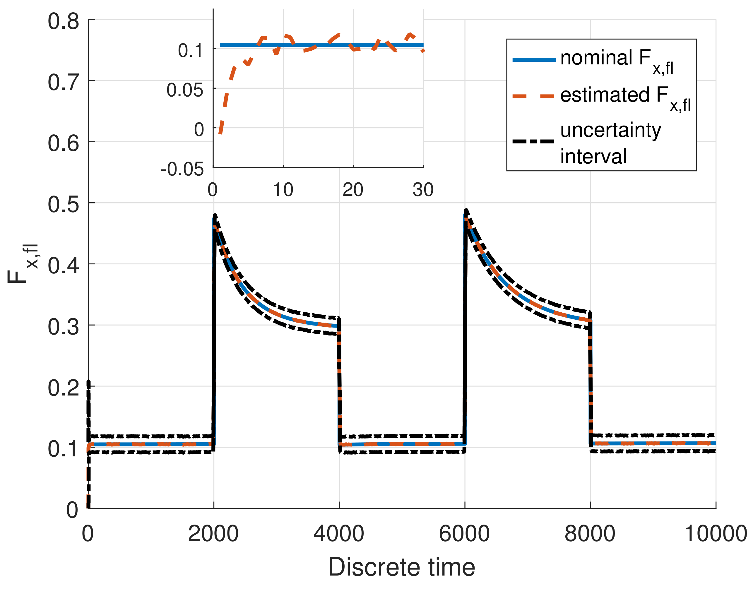
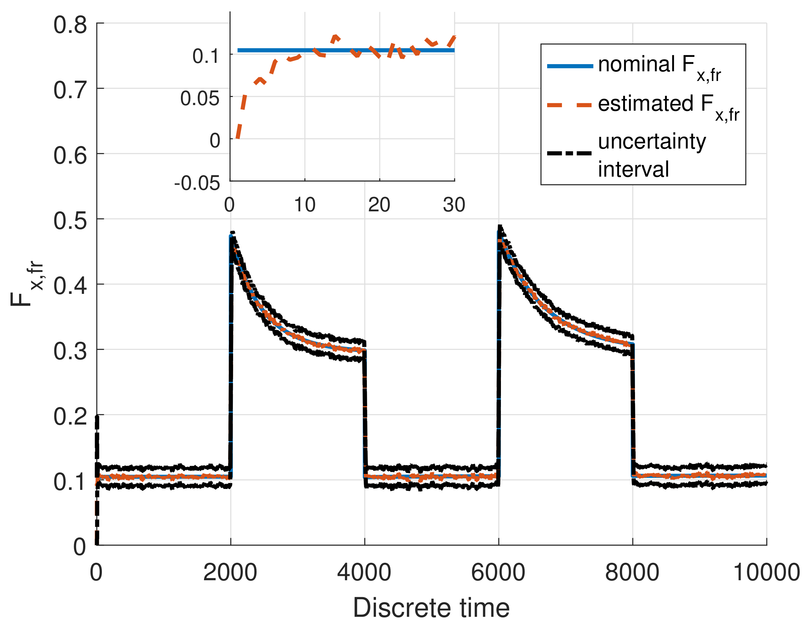
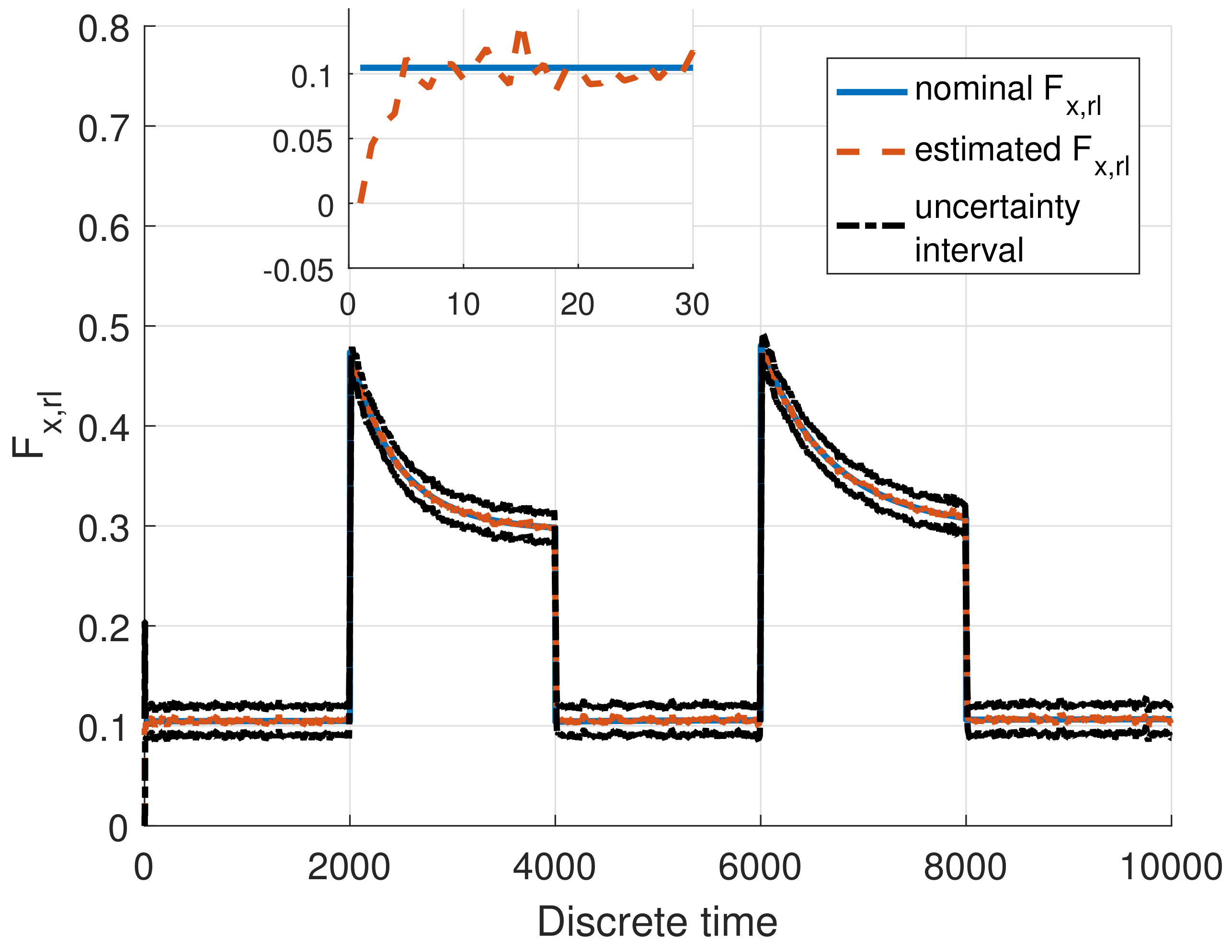
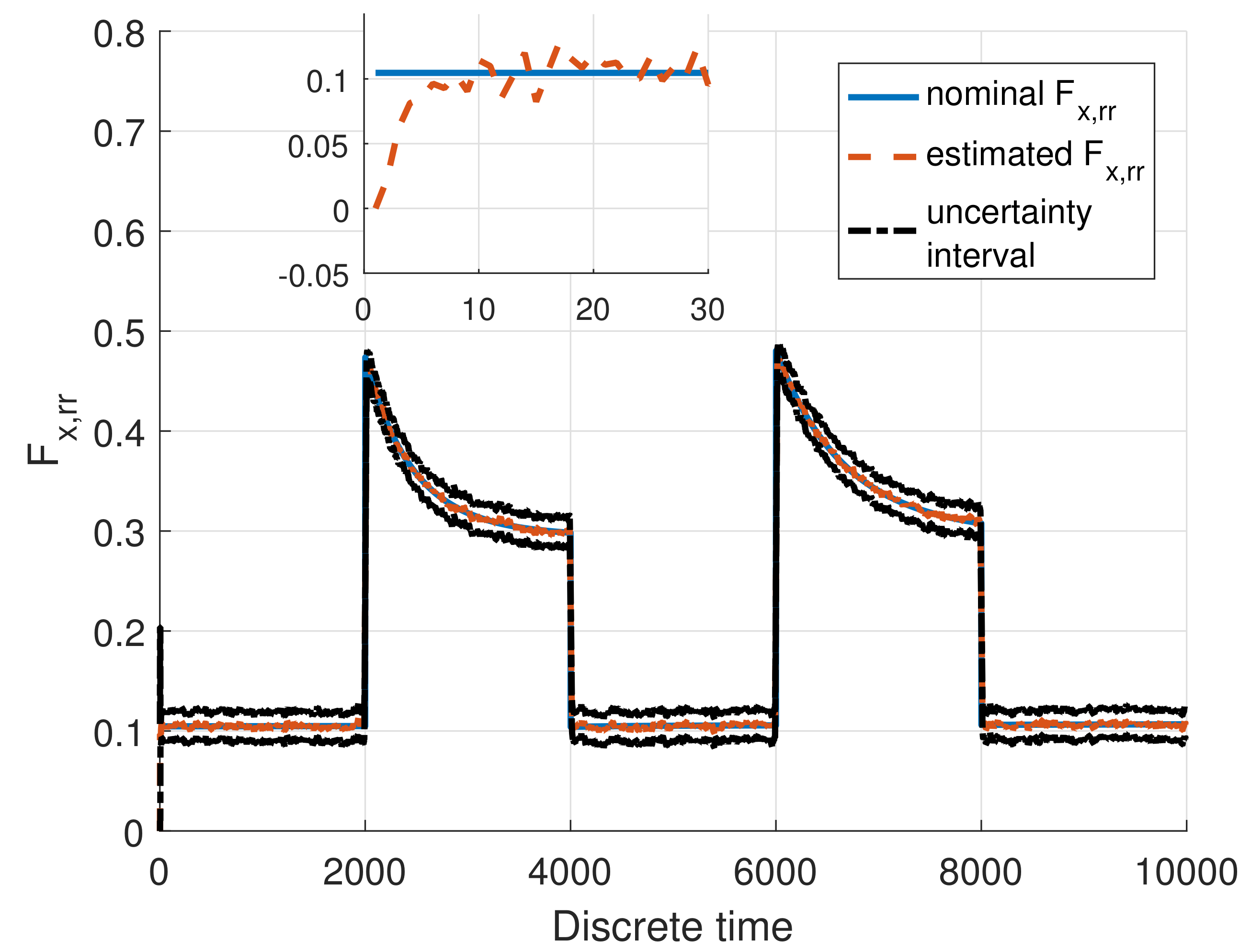
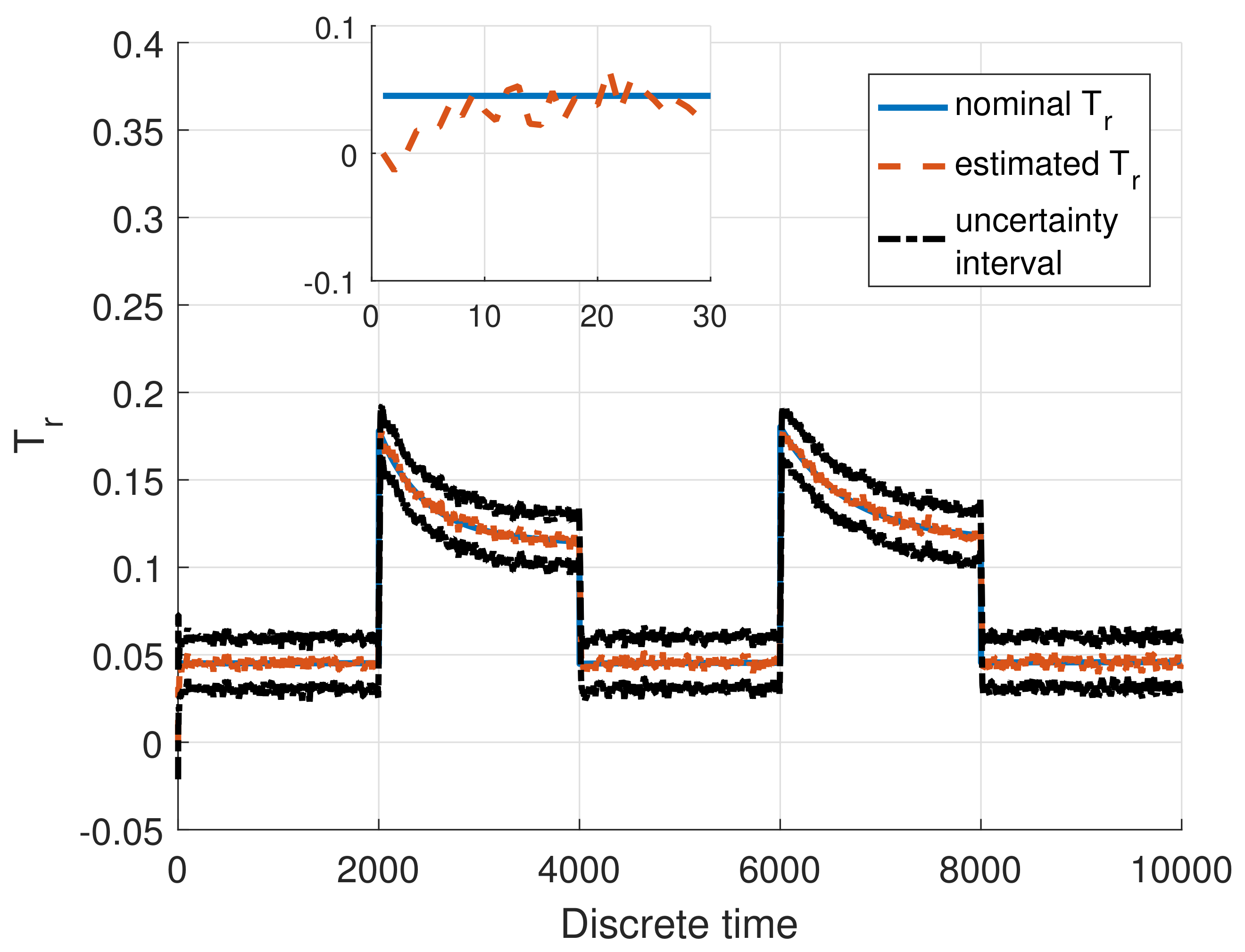
Following the above defined driving scenario, Figure 4, Figure 5, Figure 6 and Figure 7 present the longitudinal forces calculated with the model (nominal case) and their counterparts obtained with a set of measurements available from the AGV sensors. Note also that the plots show uncertainty intervals calculated according to (63) and (64). Analogous results are obtained for the torque, which are presented in Figure 8.

As it was mentioned in Section 6, the proposed estimation strategy can be also realized with an alternative approach, which employs the descriptor-like form [28] of the system (40). For that purpose, it is necessary to use the small angle approximation for which parameter $p_r$ in (38) is set to zero. This means that this matrix is constant ${\mathit{G}}_k=\mathit{G}$ and a singular one. Figure 9 presents a comparison between the nominal force and the descriptor-based one. Note that the results are presented for $F_{x,fr}$; however, a similar effect can be observed for the remaining forces as well as the torque. Indeed, it can be observed that the descriptor-based approach does not perform satisfactorily. Taking into account the results obtained with the proposed approach, it can be concluded that the developed strategy can be perceived as a very good tool for estimating AGV longitudinal forces as well as the torque.

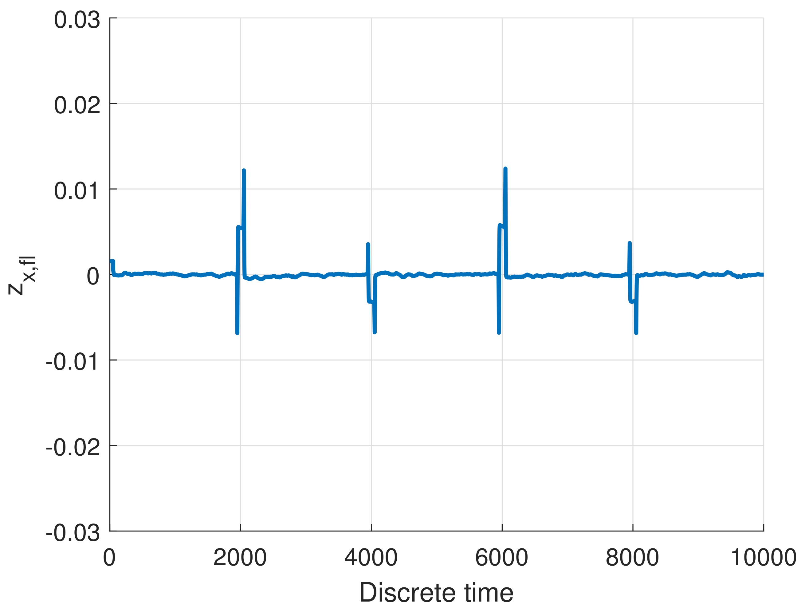
It can be observed that the estimates are consistent with the longitudinal forces and torques obtained by the model and the forces are equally distributed among the wheels. Indeed, Figure 10 presents the residual $z_{x,fl}$, which clearly indicates that it is close to zero for the fault-free case except for some transient phases corresponding to fast changes in the steering angle. As can be seen in Figure 10, the residual centers nicely close to zero, clearly indicating the fault-free, nominal case. The same situation occurs for the remaining wheels as well as the torque, which are omitted.

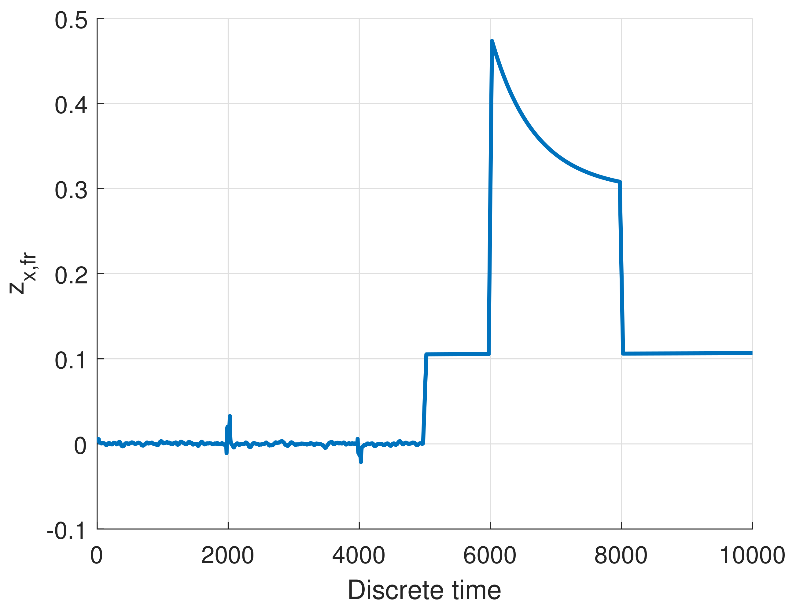
If the virtual sensors operate properly in the fault-free case, then their performance can be evaluated in the fault case. For that purpose, the AGV was steered to two overlapping surfaces in a manner that one of the wheels was hanging in the air. In particular, the front right wheel had no contact with the surface, and, hence, it did not generate the longitudinal force appropriately. This unappealing phenomenon was immediately indicated by residual $z_{x,fr},$ which is shown in Figure 11.

9. Conclusions

The main research question to be answered was whether it is possible to design reliable virtual sensors for longitudinal forces and torques of automated guided vehicles based on a quadratic boundedness approach. For this purpose, a novel approach using quadratic boundedness was proposed. This approach allows to include bounded disturbances and was implemented on a prototype AGV under development at the University of Applied Sciences Ravensburg-Weingarten. This AGV disposes of a unique design that allows unlimited maneuvering possibilities and driving on uneven terrain. However, the steering mechanism requires reliable sensor information. This information can be enhanced using virtual sensors. In contrast to several approaches from literature, the novel approach towards virtual sensors does not require the utilization of sophisticated and somewhat unreliable tire models. The use of these models frequently impairs the estimation performance and changes the whole estimation problem to a nonlinear one. The application of the approach resulted in the insight that the generated estimates are consistent with the longitudinal forces and torques obtained by a proven reference model and that the estimate immediately generates residuals in faulty cases, thus allowing effective fault detection.

References

- Schulze, L.; Wullner, A. The Approach of Automated Guided Vehicle Systems. In Proceedings of the IEEE International Conference on Service Operations and Logistics, and Informatics (SOLI ’06), Shanghai, China, 21–23 June 2006. [Google Scholar]
- Wu, S.; Wu, Y.; Chi, C. Development and Application Analysis of AGVs in Modern Logistics. Rev. Fac. Ing. 2015, 32, 380–386. [Google Scholar]
- Seybold, L.; Witczak, M.; Majdzik, P.; Stetter, R. Towards robust predictive fault–tolerant control for a battery assembly system. Int. J. Appl. Math. Comput. Sci. 2015, 25, 849–862. [Google Scholar] [CrossRef]
- Pratama, P.; Jeong, J.H.; Jeong, S.K.; Kim, H.K.; Kim, H.S.; Yeu, T.K.; Hong, S.B.; Kim, S. Adaptive Backstepping Control Design for Trajectory Tracking of Automatic Guided Vehicles. In AETA 2015: Recent Advances in Electrical Engineering and Related Sciences. Lecture Notes in Electrical Engineering; Springer: Cham, Switzerland, 2016; Volume 371. [Google Scholar]
- Ponsart, J.C.; Theilliol, D.; Aubrun, C. Virtual sensors design for active fault tolerant control system applied to a winding machine. Control Eng. Pract. 2010, 18, 1037–1044. [Google Scholar] [CrossRef]
- Witczak, M. Fault Diagnosis and Fault-Tolerant Control Strategies for Non-Linear Systems; Springer: Cham, Switzerland, 2014; Volume 266, p. 229. ISBN 978-3-319-03013-5. [Google Scholar]
- Ding, S. Model-Based Fault Diagnosis Techniques: Design Schemes, Algorithms and Tools; Springer: Berlin/Heidelberg, Germany, 2008; p. 920. [Google Scholar]
- Zhang, H. Software Sensors and Their Applications in Bioprocess; Springer: Berlin/Heidelberg, Germany, 2009. [Google Scholar]
- Srinivasarengan, K.; Ragot, J.; Aubrun, C.; Maquin, D. An adaptive observer design approach for discrete-time nonlinear systems. arXiv, 2017; arXiv:1704.05388. [Google Scholar]
- Aouaouda, S.; Chadli, M.; Shi, P.; Karimi, H. Discrete-time H_/H-inf sensor fault detection observer design for nonlinear systems with parameter uncertainty. Int. J. Robust Nonlinear Control 2015, 25, 339–361. [Google Scholar] [CrossRef]
- López-Estrada, F.; Ponsart, J.; Astorga-Zaragoza, C.; Camas-Anzueto, J.; Theilliol, D. Robust sensor fault estimation for descriptor-lpv systems with unmeasurable gain scheduling functions: Application to an anaerobic bioreactor. Int. J. Appl. Math. Comput. Sci. 2015, 25, 233–244. [Google Scholar] [CrossRef]
- Foo, G.; Zhang, X.; Vilathgamuwa, M. A sensor fault detection and isolation method in interior permanent-magnet synchronous motor drives based on an extended Kalman filter. IEEE Trans. Ind. Electron. 2013, 60, 3485–3495. [Google Scholar] [CrossRef]
- Pourbabaee, B.; Meskin, N.; Khorasani, K. Sensor fault detection, isolation, and identification using multiple-model-based hybrid Kalman filter for gas turbine engines. IEEE Trans. Control Syst. Technol. 2016, 24, 1184–1200. [Google Scholar] [CrossRef]
- Cai, J.; Ferdowsi, H.; Sarangapani, J. Model-based fault detection, estimation, and prediction for a class of linear distributed parameter systems. Automatica 2016, 66, 122–131. [Google Scholar] [CrossRef]
- Alessandri, A.; Baglietto, M.; Battistelli, G. Design of state estimators for uncertain linear systems using quadratic boundedness. Automatica 2006, 42, 497–502. [Google Scholar] [CrossRef]
- Kiencke, U.; Nielsen, L. Automotive Control Systems; Springer: Berlin/Heidelberg, Germany, 2000. [Google Scholar]
- Rajamani, R.; Phanomchoeng, G.; Piyabongkarn, D.; Lew, J. Algorithms for real-time estimation of individual wheel tire-road friction coefficients. IEEE/ASME Trans. Mechatron. 2012, 17, 1183–1195. [Google Scholar] [CrossRef]
- Milanese, M.; Novara, C.; Hsu, K.; Poolla, K. The filter design from data (FD2) problem: Nonlinear set membership approach. Automatica 2009, 45, 2350–2357. [Google Scholar] [CrossRef]
- Poggi, T.; Rubagotti, M.; Bemporad, A.; Storace, M. High-speed piecewise affine virtual sensors. IEEE Trans. Ind. Electron. 2012, 59, 1228–1237. [Google Scholar] [CrossRef]
- Novara, C.; Ruiz, F.; Milanese, M. Direct filtering: A new approach to optimal filter design for nonlinear systems. IEEE Trans. Autom. Control 2013, 58, 86–99. [Google Scholar] [CrossRef]
- Rubagotti, M.; Poggi, T.; Oliveri, A.; Pascucci, C.; Bemporad, A.; Storace, M. Low-complexity piecewise-affine virtual sensors: Theory and design. Int. J. Control 2014, 87, 622–632. [Google Scholar] [CrossRef]
- Pazera, M.; Buciakowski, M.; Witczak, M. Robust multiple sensor fault-tolerant control for dynamic non-linear systems: application to the aerodynamical twin-rotor system. Int. J. Appl. Math. Comput. Sci. 2018, 28. [Google Scholar]
- Ding, B. Constrained robust model predictive control via parameter-dependent dynamic output feedback. Automatica 2010, 46, 1517–1523. [Google Scholar] [CrossRef]
- Ziemniak, P.; Stania, M.; Stetter, R. Mechatronics Engineering on the Example of an Innovative Production Vehicle. In Proceedings of the 17th International Conference on Engineering Design (ICED’09), Palo Alto, CA, USA, 24–27 August 2009; Volume 1, pp. 61–72. [Google Scholar]
- Stetter, R.; Paczynski, A. Intelligent Steering System for Electrical Power Trains. In Proceedings of the Emobility-Electrical Power Train, Leipzig, Germany, 8–9 November 2010; pp. 1–6. [Google Scholar]
- Witczak, M.; Buciakowski, M.; Puig, V.; Rotondo, D.; Nejjari, F. An LMI approach to robust fault estimation for a class of nonlinear systems. Int. J. Robust Nonlinear Control 2015. [Google Scholar] [CrossRef] [Green Version]
- Ishihara, J.; Terra, M.; Campos, J. Robust Kalman filter for descriptor systems. IEEE Trans. Autom. Control 2006, 51, 1354–1354. [Google Scholar] [CrossRef]
- Rodrigues, M.; Hamdi, H.; Theilliol, D.; Mechmeche, C.B.B. Actuator fault estimation based adaptive polytopic observer for a class of LPV descriptor systems. Int. J. Robust Nonlinear Control 2015, 25, 673–688. [Google Scholar] [CrossRef]
Figure 1.
Automated guided vehicle (AGV).
Figure 2.
Steering system. COG: center of gravity.
Figure 3.
Suspension system.
Figure 4.
Nominal and estimated .
Figure 5.
Figure 6.
Figure 7.
Figure 8.
Figure 9.
Estimate of with the descriptor-LPV (Linear Parameter-Varying) approach (dashed line).
Figure 10.
Residual for the fault-free case.
Figure 11.
Residual for the faulty case.