Article

Rapid and Quantitative Determination of Soil Water-Soluble Nitrogen Based on Surface-Enhanced Raman Spectroscopy Analysis

1
College of Biosystems Engineering and Food Science, Zhejiang University, Hangzhou 310058, China
2
Key Laboratory of Spectroscopy Sensing, Ministry of Agriculture, P.R. China
3
College of Automation, Zhongkai University of Agriculture and Engineering, Guangzhou 510225, China
4
State Key Laboratory of Modern Optical Instrumentation, Zhejiang University, Hangzhou 310058, China
*
Authors to whom correspondence should be addressed.
Appl. Sci. 2018, 8(5), 701; https://doi.org/10.3390/app8050701
Submission received: 9 March 2018 / Revised: 26 April 2018 / Accepted: 27 April 2018 / Published: 2 May 2018
(This article belongs to the Section Optics and Lasers)

Abstract

:

Featured Application

Rapidly and quantitatively determine soil water-soluble nitrogen based on surface-enhanced Raman spectroscopy.

Abstract

An accurate and rapid determination of soil water-soluble nitrogen is conducive to scientific fertilization in precision agriculture. Surface-enhanced Raman spectroscopy (SERS) is a highly sensitive fingerprint with the advantages of simple operation and high detection efficiency. In this paper, partial least squares (PLS), principal components analysis (PCA), and least squares supports vector machine (LS-SVM) were applied to analyze the relationship between soil water-soluble nitrogen concentration and SERS. The results showed that the SERS-enhancing effect based on Opto Trace Raman 202 (OTR 202) was better than that of silver nanosubstrate and gold nanosubstrate. In addition, the prediction accuracy of soil water-soluble nitrogen in PLS was the highest ( R p 2 = 0.91 ,   RMSE p = 8.76   mg / L , R P D = 3.00 ) when the original spectra were preprocessed with first-derivative. Moreover, 1028, 1370, 1436, and 1636 cm−1 could be determined as characteristic peaks of soil water-soluble nitrogen, the association between soil water-soluble nitrogen concentration and a SERS intensity of 1370 cm−1 was the highest   ( R p 2 = 0.94 ) , and the regression equation was y = 93.491x + 1771.5. Beyond that, the prediction accuracy of distinguishing between a low soil water-soluble nitrogen concentration (22.7–63.7 mg/L) and a high soil water-soluble nitrogen concentration (70.5–118.3 mg/L) based on PCA and LS-LVM was 86.67%. In conclusion, soil water-soluble nitrogen could be detected rapidly and quantitatively using SERS, which was beneficial to provide a rapid, accurate, and reliable scheme for scientific and precise fertilization.

1. Introduction

Soil nitrogen is the key parameter supporting plant growth and development. There are many forms of nitrogen in soil, with soil water-soluble nitrogen being one of the more important substances that plants can absorb directly [1]. However, the content of water-soluble nitrogen in soil is low. Therefore, it is necessary to accurately determine soil water-soluble nitrogen, so as to provide a scientific basis for rational fertilization [2]. The acid hydrolysis [3], the alkali hydrolysis diffusion [4], and the alkaline hydrolysis distillation [5] methods are the traditional chemical methods for the determination of soil water-soluble nitrogen. Although these methods are highly sensitive, the disadvantages of tedious measurement, long detection time, and expensive reagent limit their development [6]. In recent years, spectral technology has been widely applied to soil nitrogen detection, among which near infrared spectroscopy has certain advantages and application prospects [7,8]. However, near infrared spectroscopy cannot overcome the effect of moisture on soil nitrogen detection, which limits its practical application in nitrogen detection to a certain extent, especially the detection of water soluble and hydrolytic nitrogen [9,10].
Surface-enhanced Raman spectroscopy (SERS) has attracted wide attention in recent years. The principle is that the molecular signals in the chemical compound can be enhanced when the detected materials surface adsorb some nanoscale rough metals (such as gold, silver, and copper) [11]. Beside this, SERS also has the advantages of simple pretreatment, convenient equipment, and fast detection speed, which makes it suitable for the rapid screening of complex compounds [12]. Some researchers have applied SERS to nitrogen molecular analysis. El Torres et al. [13] successfully applied SERS based on silver colloids to trace the determination of nitrogen-containing drugs. Li et al. [14] monitored nitrogen assimilation at the levels of large cells and single cells by SERS combined with the stable isotope detection technique. The results indicated that the nondestructive approach could identify active nitrogen assimilation cells for genomic analysis and provide a theoretical basis for further comprehending the nitrogen metabolism of environmental microorganisms. Vlasov et al. [15] found that the first and second order Raman spectroscopy (RS) of disordered graphite and polyacetylene could be applied to detect and analyze different nitrogen content using 514.5 and 413.1 nm laser excitation. Furthermore, the adsorption and orientation of nitrogen compounds on the surface of iron in an acidic solution by SERS was studied and discussed in Uehara’s research [16].
In the study of soil water-soluble nitrogen in agriculture, many domestic and foreign scholars have carried out relevant research. However, there are few studies on the application of SERS in the determination of soil water-soluble nitrogen. In this paper, the purpose of this study is to apply the SERS technique to detect soil water-soluble nitrogen quickly and accurately. Moreover, the enhancing effects of silver colloid, gold colloid, and Opto Trace Raman 202 (OTR 202) were compared. As a result, we established the regression equation between SERS characteristic peaks intensity and soil water-soluble nitrogen, which helped to improve the efficiency of soil water-soluble nitrogen detection and provide a scientific guidance for urea fertilization.

2. Materials and Methods

2.1. Experimental Materials and Sample Preparation

The experimental soil samples were acidic red soil which was collected from the Qingyuan county, Zhejiang province, China (N 34°44′, E 127°45′). Urea is the main source of soil water-soluble nitrogen in agriculture. In this experiment, the process of specific sample preparation was as follows. First, soil samples were air-dried and sieved through 80 mesh sifters (0.18 mm). Second, 15 samples (each sample weighing 5 g) were accurately weighed, mixed with 5 mL urea solutions respectively, and stirred adequately. Third, each soil sample was placed in a 40 °C oven for 48 h and then mixed with 100 mL distilled water and stirred. Fourth, all soil samples were placed in a 20 °C environment for 24 h. Finally, soil sample solutions were filtered through 0.22 μm organic membranes and the supernatant was obtained. The final soil water-soluble nitrogen concentrations were 22.7, 29.6, 36.4, 43.2, 50, 56.7, 63.7, 70.5, 77.3, 84.1, 91, 97.8, 104.6, 111.4, and 118.3 mg/L. There were eight samples for each concentration and 120 samples in total.

2.2. Nano-Sol Substrate Preparation

The preparation of silver colloid was established on the basis of the Lee–Meisel trisodium citrate heating reduction method [17]. The process of silver nanosubstrate preparation was as follows. First, a silver nitrate solution (180 mg/L) was heated at a high temperature on a constant-temperature magnetic stirrer. Second, 1% trisodium citrate solution was dropwise added into silver nitrate solution and then stirred at 200 rpm. Third, heating and stirring was stopped when the solution turned grey-green within 25 min. Fourth, when the heating temperature dropped, the silver nitrate solution was poured into a centrifuge tube and stored in the dark at 4 °C after repeating purification.
In this experiment, we have made a slight improvement on the preparation of nanogold through the heating reduction of trisodium citrate [18]. The preparation process of gold nanosubstrate was as follows. First, the chloroauric acid solution (50 mg/L) was heated to 120 °C in a constant-temperature magnetic stirrer; then, 4 mL citric acid trisodium sodium solution (5 mg/mL) was added to the above solution. Second, the solution was stirred at 100 rpm until the color of gold sol turned wine red. Third, when the heating temperature dropped, the gold nitrate solution was poured into a centrifuge tube and stored in the dark at 4 °C after repeating purification.
In addition, in this paper, the OTR 202 nanomaterials produced by OptoTrace Technologies, Inc. (Suzhou, China) was also used in this paper. It has the advantages of an obvious enhancement effect, uniform nanoparticles, and low cost.

2.3. Experimental Instrument

The experimental instruments mainly used in this study are as follows: (1) RmTracer-200-HS portable Raman spectrometer, combined with a 785 nm excitation wavelength diode-stabilized stimulator (Opto Trace Technologies, Inc., Silicon Valley, CA, USA); (2) FA1004B electronic balance (Shanghai Shangping Instrument Co., Ltd., Shanghai, China), whose accuracy is 0.1 mg; (3) JW-1024 low-speed centrifuge (Anhui Jia Instrument and Equipment Co., Ltd., Hefei, Anhui, China), whose maximal speed is 4500 r/min; (4) Vortex-Genie 2/2T vortex mixer (Shanghai Ling Early Environmental Protection Instrument Co., Ltd., Shanghai, China); (5) Agilent 1290 Ultra Performance Liquid Chromatography Combined Photodiode Array Detector (Agilent Technologies, Santa Clara, CA, USA); (6) the column, Agilent ZORBAX SB-C18, 150 mm × 2.1 mm, 3.5 μm (Agilent Technologies, Santa Clara, CA, USA); (7) the FEI Tecnai G2 F20 S-TWIN transmission electron microscope (TEM, USA FEI Corporation, Santa Clara, CA, USA), which was used to observe the morphology of the substrates; and (8) 80-mesh sieve (Shanghai Yan Kam screen processing plant, Shanghai, China).

2.4. Raman Spectra Acquisition

Before RS data acquisition, the instrument was calibrated using a 785 nm excitation wavelength. The parameters were set as follows: a power of 200 mw, a scanning range of 200–3300 cm−1, an optical resolution of 2 cm−1, an integration time of 10 s, and an average spectral value of three times. The solid urea RS collection involved urea powder in a quartz plate with flattened glass slides, and the spectra were acquired with a matching microscope platform. The SERS collection method involved 500 μL OTR 202 (silver nanosubstrate or gold nanosubstrate), 100 μL detection solution, and 100 μL sodium chloride, which were then added into a 2 mL quartz bottle and placed in a liquid sample pool.

2.5. Spectral Preprocessing Methods

The noise caused by the equipment and the interference of the fluorescence background in the Raman signal could affect the detection results. Therefore, five pretreatment methods were applied to preprocessing the original Raman spectra in this paper [19]. Among them, the Savitzky–Golay (S–G) smoothing algorithm uses a weighted average method to quantify the data in the moving window by polynomial least squares fitting, which emphasizes the central role of the center point [20]. The basic idea of the multiplicative scatter correction (MSC) algorithm is to use an ideal spectrum to represent the spectrum of all samples and to correct the original spectra with the slope and intercept of linear equations [21]. The principle of the standard normal variation (SNV) algorithm is that the scattering intensity values of each wavelength point satisfies a certain distribution in each spectrum, and the spectral correction was carried out according to this assumption [22]. The idea of the de-trending (DT) algorithm is that the spectral absorbance and wavelength are first fitted into a trend line d according to the polynomial; then, the trend line d is subtracted from the original spectra x to achieve the effect of this trend [23]. The first-derivative can eliminate the interference from other backgrounds and distinguish the overlapping peaks in the spectrum, which improves spectral resolution, sensitivity, and the signal-to-noise ratio of the spectra to a certain extent [24].

2.6. Modeling Methods

Partial least squares (PLS) is the most widely used regression modeling method in spectral data analysis due to its flexibility and reliability in dealing with redundant spectral data. In the PLS model, the spectral matrix is decomposed first, and the main principal component variables are obtained; then, the contribution rate of each principal component is calculated. The flexibility of PLS makes it possible to establish a regression model in the case where the number of samples is less than the number of variables. In this study, the PLS model was established with the spectral data as X and the measured soil water-solution content as Y, whose best principal factor was determined by the root mean square error of cross validation (RMSECV) [25].
Principal component analysis (PCA) is a statistical method based on the principle of maximum variance, which adopts low dimensional variables instead of the original high dimensional variables so as to achieve the purpose of reducing data dimension. The principal components of the PCA are independent of each other, which effectively eliminates the redundant information in the original data. In general, the first few principal component variables existed with large deviations, which can be used to sample and discriminate between clusters of species instead of all the variables [26].
Least squares support vector machines (LS-SVM) is a supervised learning model, whose main purpose is to find an optimal classification hyperplane to satisfy the classification requirements. The LS-SVM first maps the nonlinear training data to a higher dimensional feature space (Hilbert space), and then finds a hyperplane between positive and negative values in the high dimensional feature space. The application of LS-SVM can effectively solve the problems of a traditional neural network, such as the local minimum and overfitting. It provides an impressive performance for small samples, nonlinear high dimensional data such as machine learning problems, which has been widely used in pattern recognition; data mining, and other fields [27].
All data analysis was based on MATAB R2014a (The Math-Works, Natick, MA, USA) and OMNIC v8.2 (Infrared spectrum processing software, Thermo Fisher Scientific, Waltham, MA, USA).

2.7. Model Evaluation Index

In this experiment, the modeling effect is evaluated by the coefficient of determination (R2), the root mean square error (RMSE), and the residual predictive deviation (RPD). The coefficient of determination R2 reflects the level of intimacy between variables, the RMSE reflects the accuracy of the model, and RPD reflects the predictive ability of the model. The higher the RPD, the lower the RMSE, and the closer the R2 is to 1, the better the performance of the prediction model. In this paper, R c 2   and R p 2 represent the coefficient of the determination of the calibration set and the prediction set respectively, while RMSE c and RMSE p represent the root mean square error of the calibration set and the prediction set respectively. In addition, the RPD was suggested to be at least three for agriculture applications; while 2 < RPD <3 indicated a model with a good predictive ability; 1.4 < RPD < 2 was an intermediate model needing some improvement; and RPD < 1.4 indicated that the model had a poor predictive ability [28].

3. Results and Discussion
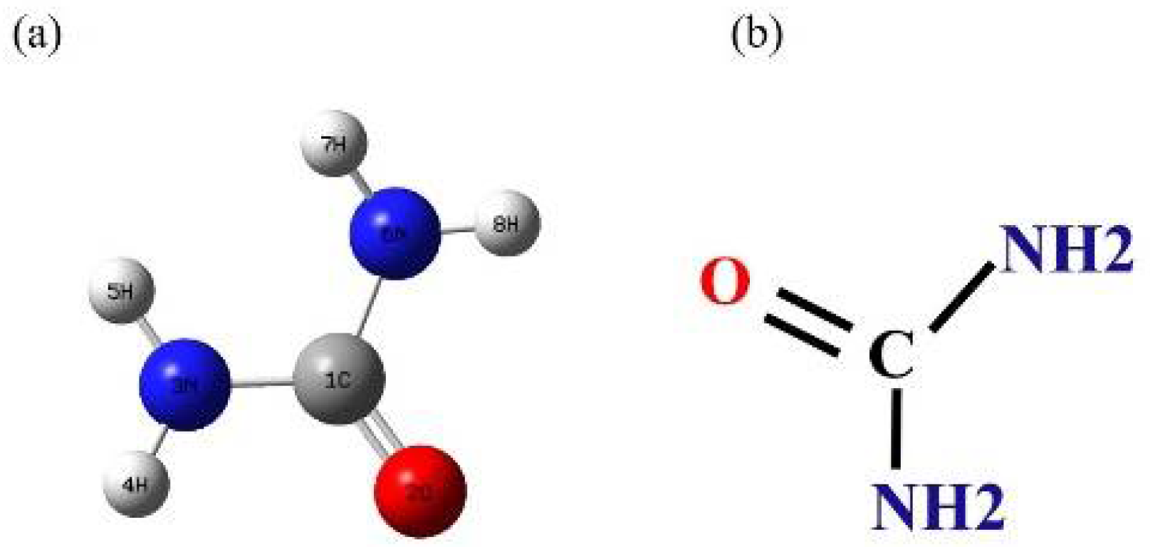
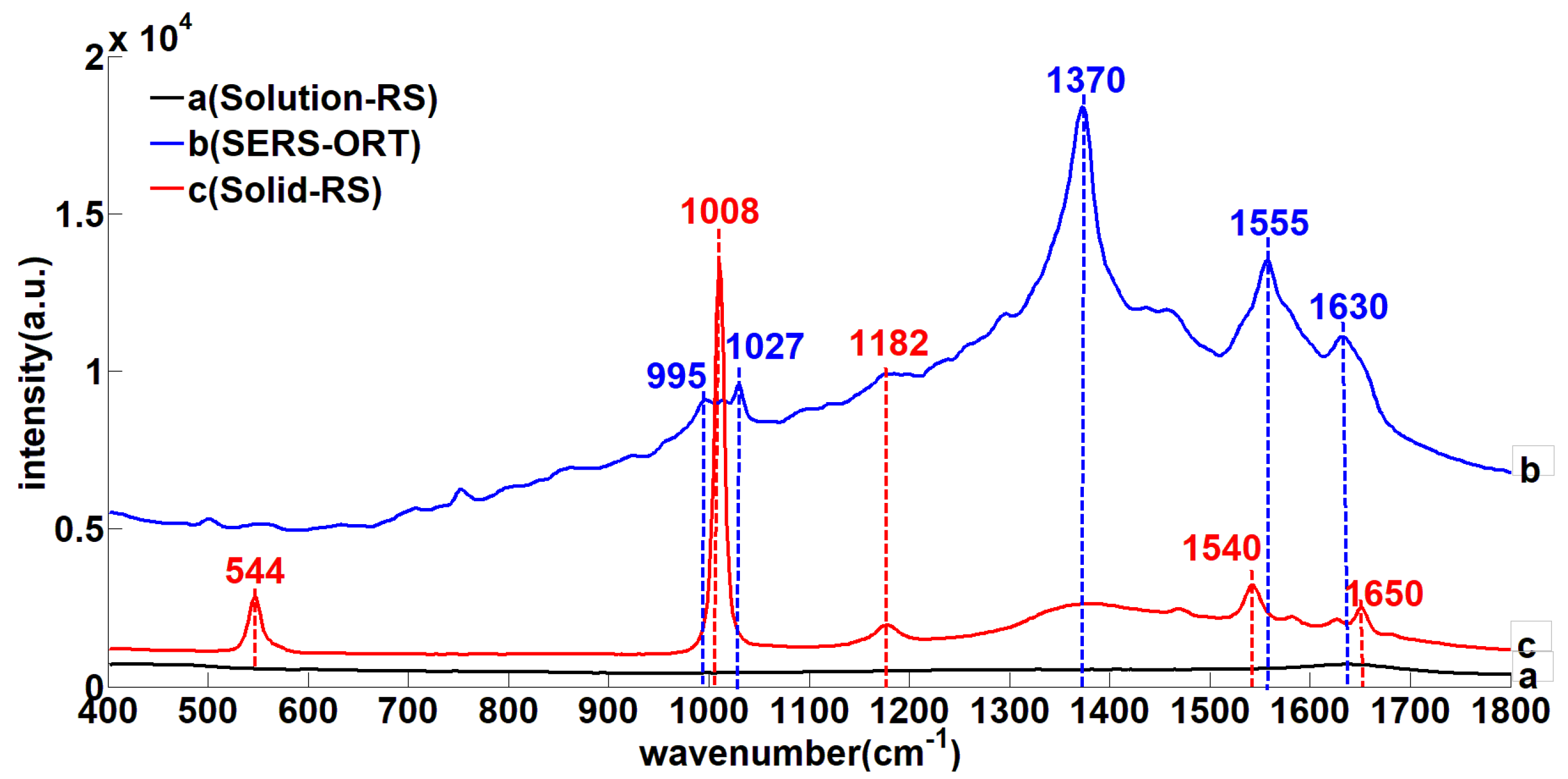
3.1. The Urea SERS

In this experiment, the water-soluble nitrogen in soil mainly came from urea. Therefore, analyzing the urea molecule and finding the assignment of Raman peaks of the urea molecule were conducive to current knowledge on the vibration forms of soil water-soluble nitrogen. Urea (molecular formula: CO(NH2)2), is mainly composed of C–N, C–H and NH2 groups with a relative molecular mass of 60.06. The urea molecular space structure and planar structure are shown in Figure 1. In order to further understand the speciation of water-soluble nitrogen, the 100 mg/L standard urea solution RS (solution-RS), 100 mg/L standard urea solution SERS, and solid RS (solid-RS) were collected. Figure 2 displays the spectral curves of solution-RS, SERS, and solid-RS.
The assignment of SERS peaks can be concluded with Figure 2 and Table 1. According to Figure 2, there were no characteristic peaks in the solution-RS curve. However, there were some significant characteristic peaks when nanoenhancers (OTR 202) were added, which suggested that nano-enhancers could improve the signal of nitrogen detection. Among them, 544 cm−1 belonged to the C–N in-plane bending, 995 cm−1 belonged to the N–H stretching vibration, 1008 and 1027 cm−1 were the C–N stretching vibration, 1182 cm−1 was the N–H in-plane bending, 1370 cm−1 was the N–H stretching vibration, 1540 and 1555 cm−1 were the C=O stretching vibration, 1630 cm−1 belonged to the N–H stretching vibration, and 1650 cm−1 was the NH2 in-plane swaying vibration. Similar results can be found in studies by Rousseau [29], Wang [30] and Duncan [31].
It can be seen that the solid-RS had obvious characteristic peaks at 544, 1008, 1176, 1540, and 1650 cm−1. The characteristic peaks at 544, 1008, and 1650 cm−1 were the special molecular vibrations in the solid. As for the SERS, the characteristic peaks at 1370 cm−1 occurred but they did not appear in solid-RS. The reason might be that the NH2 group transformed to N–H when the solid urea dissolved in water. With the exception of 1555 cm−1 (the stretching vibration of the C=O), the vibrations of the other bonds were all related to N, and their characteristic peaks in order of intensity strength were 1370, 1027, 1630, and 995 cm−1. Furthermore, the intensity strength was the highest at 1008 cm−1 in solid-RS. The reason was that the quantity of C–N in the urea molecule was the largest, and the vibration of the molecule was the greatest. In addition, the absorption intensity which was caused by the vibration of N–H at 1370 cm−1 was the strongest in SERS.

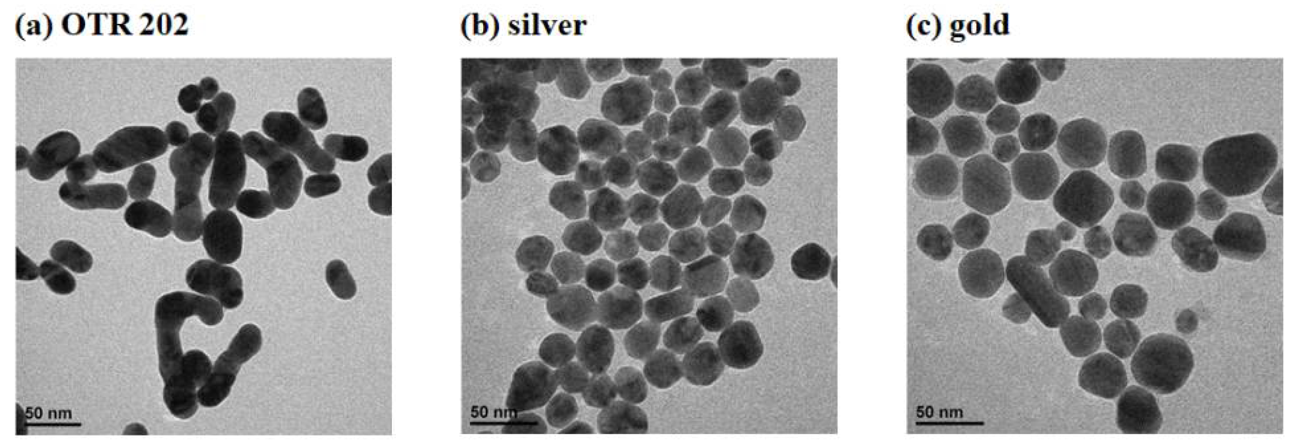
3.2. The Comparation of Three Nanoenhancers

To investigate and find the optimal nanoenhancer, the enhancement effects of OTR 202 nanosubstrate, silver nanosubstrate, and gold nanosubstrate were compared and analyzed in this study. The structure diameter of OTR 202 nanoparticles, silver nanoparticles, and gold nanoparticles were characterized by Transmission Electron Microscopy (TEM) in Figure 3a–c respectively.
As can be seen in Figure 3, the nanoparticle sizes of OTR 202, silver substrate, and gold substrate were uniform. Moreover, the gold nanoparticle size was bigger than that of the OTR 202 and the silver nanoparticle, while the nanoparticle size of OTR 202 was the smallest. The SERS values based on the OTR 202 nanosubstrate, the silver nano-substrate, and the gold nanosubstrate are shown in Figure 4a–c respectively. According to these values, the enhancement performance of the Raman peaks of OTR 202 nanosubstrate at 994, 1028, 1370, 1554, and 1636 cm−1 were superior to that of the gold substrate. In addition, the Raman peaks of 1555 and 1630 cm−1 appeared when OTR 202 was used while those two Raman peaks did not appear in the SERS combined with the gold substrate, which indicated that the enhancement of OTR 202 was better than that of the gold substrate. The reason might be that the ultraviolet characteristic absorption peaks of urea and OTR 202 nanoparticles were more similar. Thus, the surface plasmon resonance of OTR 202 can be stimulated more easily, resulting in a higher detection sensitivity [32]. As for silver nanosubstrate, although there were seven stronger Raman peaks (465, 616, 939, 1107, 1266, 1410, and 1449 cm−1) in the SERS, these peaks also occurred in the SERS of soil extract without urea (Figure 4d).This might be because the peak signals of other substances in the soil extract were amplified, which covered up the molecular vibration of soil water-soluble nitrogen. Therefore, the OTR 202 nanoparticle was selected as the enhancer in the following study.

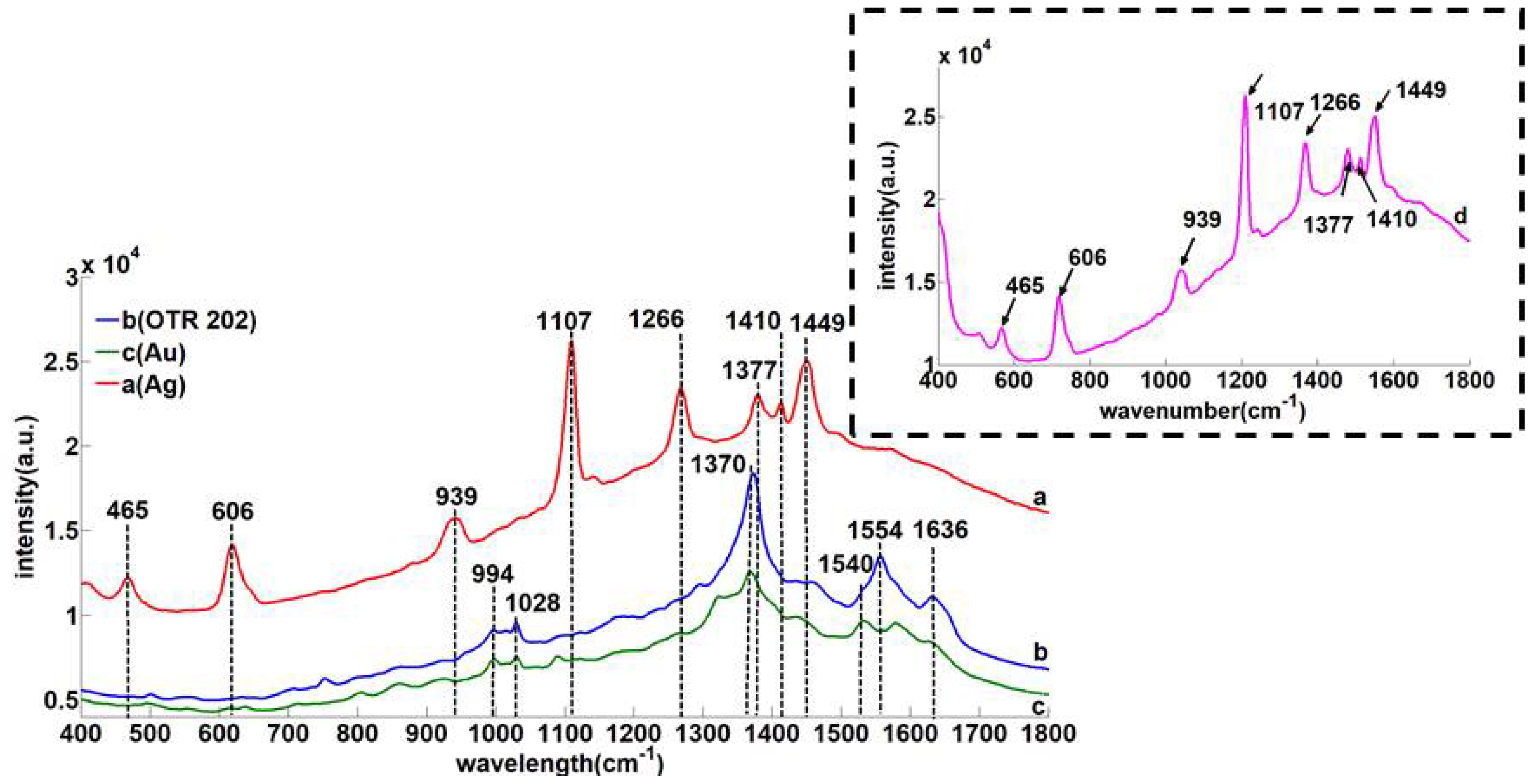
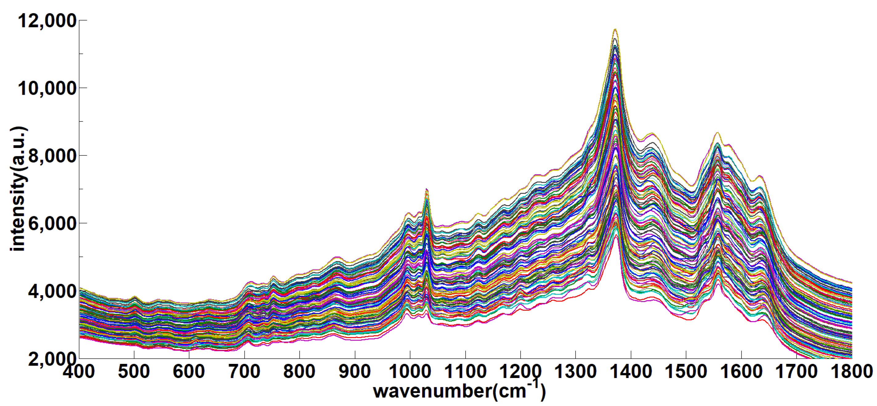
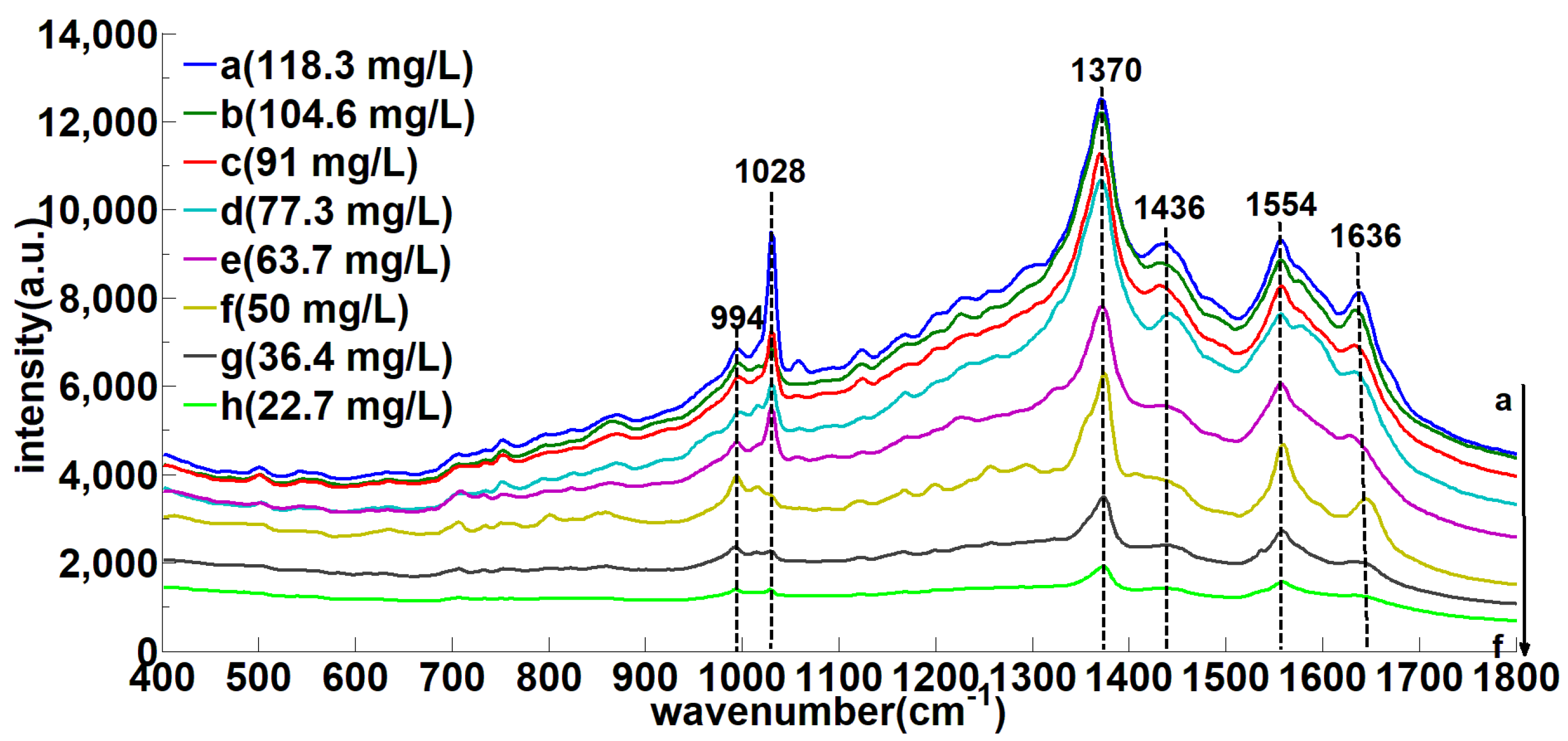
3.3. 400–1800 cm−1 Soil SERS Analysis
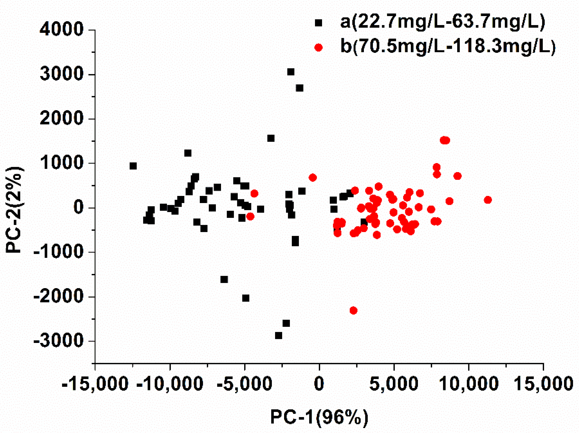
In this experiment, SERS data for 120 soil samples were collected. Figure 5 shows the 400–1800 cm−1 SERS of 120 soil samples, and Figure 6 shows eight water-soluble nitrogen concentrations (22.7, 36.4, 50, 63.7, 77.3, 91, 104.6, and 118.3 mg/L) SERS. The abscissa is the wavenumber and the ordinate is the SERS intensity.
According to Figure 5 and Figure 6, the SERS absorbance intensity decreased gradually with the decrease in soil water-soluble nitrogen concentration at the characteristic peaks of 994, 1028, 1370, 1436, 1554, and 1636 cm−1. It is indicated that those peaks could be determined as water-soluble nitrogen Raman characteristic peaks, and the SERS absorbance intensity and soil water-soluble nitrogen concentration was positively correlated.

3.4. Model Analysis

In order to eliminate spectral noise in SERS and to improve detection accuracy, 400–1800 cm−1 SERS was pretreated with four spectral preprocessing methods; then, it was modeled by PLS. In PLS, the sample set portioning based on the joint x-y distance (SPXY) method [33] was used to divide the samples into two groups, among which 80 samples were calibrated and 40 samples were predicted. Table 2 presents the modeling results of the calibration set and the prediction set with different spectral pretreatments and algorithms.
On the one hand, the prediction accuracy of soil water-soluble nitrogen ( 0.88 < R p 2 < 0.91 ,   8.76   mg / L < RMSE p < 9.36   mg / L ,   3.00 < R P D < 3.34 ) was similar when SERS was processed with those methods. Among them, the R p 2   of 1st-der was the highest. The reason might be that the first-order method could distinguish between the overlapping peaks and eliminate interference from other backgrounds, which improved the spectral resolution and separated the main characteristic peaks for quantitative analysis [34]. On the other hand, no matter which algorithm was used, the prediction accuracy of soil water-soluble nitrogen varied in a small range, indicating that the experimental results were highly reliable. All the R p 2 values reached above 0.88, and the all the RPD values were more than 3, which indicated that the determination of water-soluble nitrogen in soil using SERS was effective.

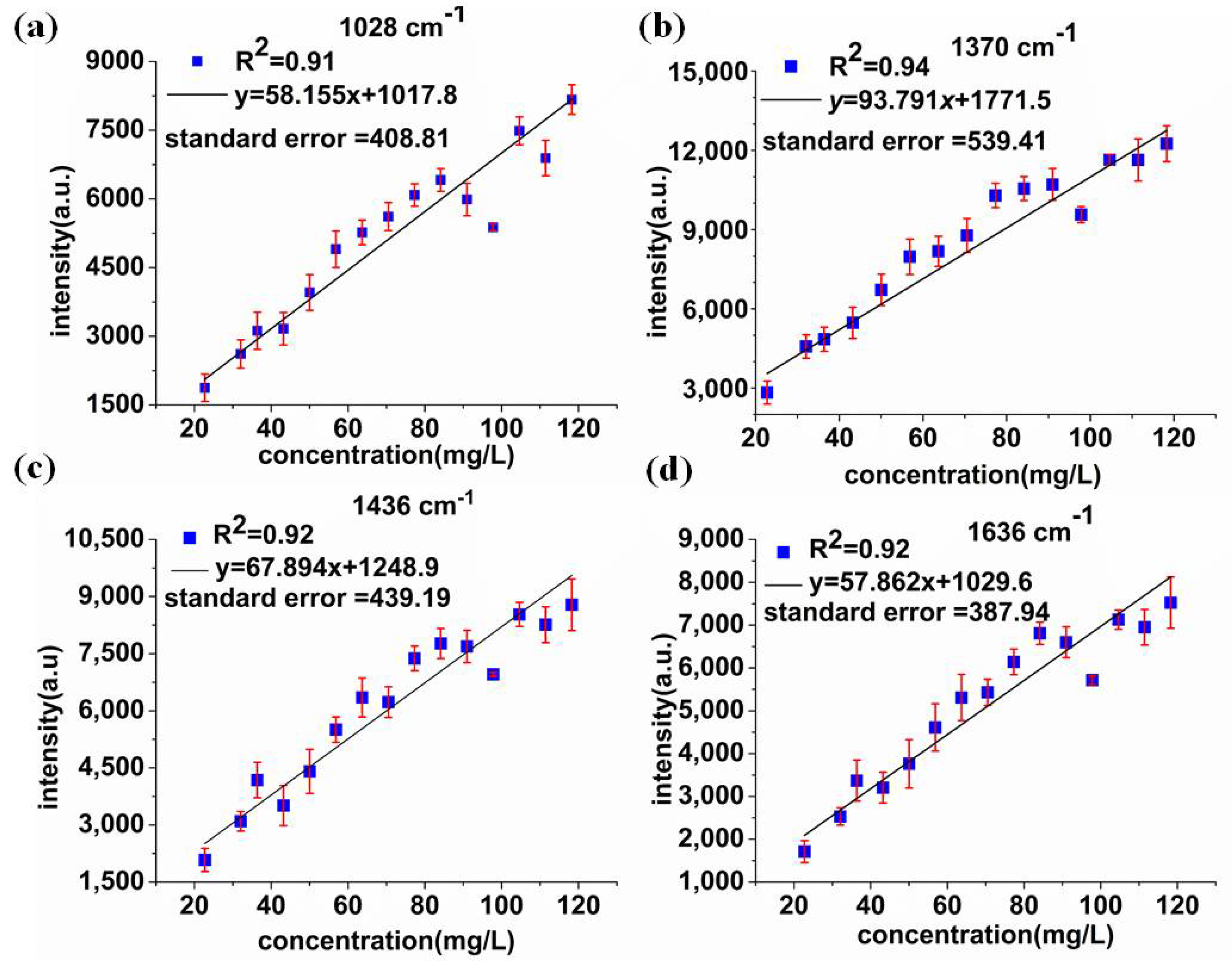
3.5. SERS Characteristic Peaks Model Analysis

Based on the above analysis, 994, 1028, 1370, 1436, and 1636 cm−1 were preliminarily selected as characteristic peaks of soil water-soluble nitrogen. The selected characteristic peaks were modeled and analyzed by PLS, whose model performances are shown in Table 3. Also, the calibration set and the prediction set was divided according to the ratio of 2:1 using the SPXY method.
The PLS models predicted by five characteristic peaks together achieved good results ( R p 2 = 0.87 ,   RMSE p = 11.03   mg / L ,   R P D = 2.56 ), which indicated that 994, 1028, 1370, 1436, and 1636 cm−1 could be integrated together to predict soil water-soluble nitrogen content accurately. However, the R p 2 of single characteristic peaks was lower than the five characteristic peaks combined. The maximal R p 2 was 0.86 using 1370 cm−1, and the corresponding RMSE p and RPD were 10.41 mg/L and 2.52 respectively. Meanwhile, the prediction result ( R p 2 = 0.77 ,   RMSE p = 13.07   mg / L ,   R P D = 1.73 ) was poor when modeled with the characteristic peak 994 cm−1, which was consistent with the relationship between the SERS absorption peak intensity and water-soluble nitrogen content. Moreover, the   R p 2   and RPD at 1028, 1436, and 1636 cm−1 all reached more than 0.80 and 2 respectively. Thus, 1028, 1370, 1436, and 1636 cm−1 could be selected as characteristic peaks of soil water-soluble nitrogen in further studies.
Based on the analysis, the regression equation between the characteristic peaks (1028, 1370, 1436, and 1636 cm−1) and the soil water-soluble nitrogen concentration was established. The fifteen point in each figure was the average SERS of fifteen different soil water-soluble nitrogen concentrations, the abscissa was the soil water-soluble nitrogen concentration, and the ordinate was the SERS intensity. The regression results are shown in Figure 7.
Figure 7a–d display the linear regression relation at 1028, 1370, 1436, and 1636 cm−1 respectively, where the coefficient of determination (R2 = 0.94) at 1370 cm−1 was the highest and the regression equation was y = 93.491x + 1771.5, which was related to the SRES peaks intensity in different Raman peak positions. The coefficient a of x was from 57.862 to 93.791, the constants b ranged from 1017.8 to 1771.5, and the standard error was from 378.94 to 539.41. The R2 of all linear regression equations was higher than 0.9, which indicated that the soil water-soluble nitrogen could be detected by those SERS characteristic peak intensities.
Given the division standard of soil water-soluble nitrogen in China [35] and the combination with the soil water-soluble nitrogen concentration in this experiment, the soil water-soluble nitrogen concentration was divided into low concentration (22.7–63.7 mg/L) and high concentration (70.5–118.3 mg/L) to analyze. PCA was used to cluster the samples, and LS-SVM was applied for classification based on two principal components and four characteristics peaks. The total number of samples was 120, and the ratio between the calibration set and the prediction set was 5:3 using SPXY. Figure 8 presents the schematic diagram principal component analysis, and the LS-SVM predictive results are shown in Table 4.
It can be seen from Figure 8 that when the soil water-soluble nitrogen concentrations were divided into two categories, the principal components 1 (PC-1) and the principal component 2 (PC-2) were accumulated to express 98% of the original information. The results of clustering were good, where the accuracy rate of the calibration set for identifying low concentrations and high concentrations was 100%, and the accuracy of the prediction set was 86.67%. It indicated that SERS could distinguish the level of soil water-soluble nitrogen concentrations well. Among them, the accuracy of identifying low soil water-soluble nitrogen concentrations and high soil water-soluble nitrogen concentrations were 90.48% and 83.33% respectively. The reason might be that the concentration gap between 63.7 mg/L and 70.5 mg/L was relatively small, which may lead to the misjudgment.

4. Conclusions

In this paper, SERS was initially applied to detect soil water-soluble nitrogen. The conclusions were as follows: (1) soil water-soluble nitrogen could effectively be determined using SERS based on OTR 202; (2) 1028, 1370, 1436, and 1636 cm−1 could be determined as characteristic peaks of soil water-soluble nitrogen, with the best relevance occurring at 1370 cm−1 and the regression equation being y = 93.491x + 1771.5; (3) SERS could sufficiently distinguish the level of soil water-soluble nitrogen concentration, and the accuracy was 86.67%, which was helpful in improving the efficiency of soil water-soluble nitrogen detection and providing a scientific guidance for urea fertilization.

Author Contributions

This work presented here was carried out through collaborations among all authors. T.D. and P.N. conceived the idea. S.X., Y.H., Y.T., L.L., F.Q. and S.L. worked together on associated data and carried out the experimental work. T.D. and P.N. drafted the manuscript. S.X., Y.H., Y.T., L.L., F.Q. and S.L. provided their experience and co-wrote the paper with T.D. and P.N.. All authors contributed, reviewed and improved the manuscript.

Acknowledgments

This work is supported in part by National keypoint research and invention program of the thirteenth (2016YFD0700304) and Natural Science Foundations of China (Grant No. 61405175).

Conflicts of Interest

The authors declare no conflict of interest.

References

  1. Anderson, R.H.; Fuhlendorf, S.D.; Engle, D.M. Soil water-soluble nitrogen Availability in Tallgrass Prairie Under the Fire–Grazing Interaction. Rangel. Ecol. Manag. 2006, 59, 625–631. [Google Scholar] [CrossRef]
  2. Veuger, B.; Oevelen, D.V.; Middelburg, J.J. Fate of microbial nitrogen, carbon, hydrolysable amino acids, monosaccharides, and fatty acids in sediment. Geochim. Cosmochim. Acta 2012, 83, 217–233. [Google Scholar] [CrossRef]
  3. Bondeson, D.; Mathew, A.; Oksman, K. Optimization of the isolation of nanocrystals from microcrystalline cellulose by acid hydrolysis. Cellulose 2006, 13, 171. [Google Scholar] [CrossRef]
  4. Vozniuk, S.T.; Truskavets’Kyi, R.S. Methods of agrochemical analysis of peat soils. Ahrokhimiia Hruntozn 1972, 21, 18–24. [Google Scholar]
  5. Cherlo, S.K.R.; Devaki, K.; Pushpavanam, S. Phase transfer catalysis of alkaline hydrolysis of n-butyl acetate: Comparison of performance of batch and micro-reactors. Chem. Eng. Proc. 2010, 49, 484–489. [Google Scholar] [CrossRef]
  6. Önal, A. A review: Current analytical methods for the determination of biogenic amines in foods. Food Chem. 2007, 103, 1475–1486. [Google Scholar] [CrossRef]
  7. Bevilacqua, M.; Bucci, R.; Materazzi, S.; Marini, F. Application of near infrared (NIR) sensors coupled to chemometrics for dried egg-pasta characterization and egg content quantification. Food Chem. 2013, 140, 726–734. [Google Scholar] [CrossRef] [PubMed]
  8. Filippi, J.J.; Belhassen, E.; Baldovini, N.; Brevard, H.; Meierhenrich, U.J. Qualitative and quantitative analysis of vetiver essential oils by comprehensive two-dimensional gas chromatography and comprehensive two-dimensional gas chromatography/mass spectrometry. J. Chromatogr. A 2013, 1288, 127–148. [Google Scholar] [CrossRef] [PubMed]
  9. He, Y.; Xiao, S.P.; Nie, P.C.; Dong, T.; Qu, F.F.; Lin, L. Research on the optimum water content of detecting soil nitrogen using near infrared sensor. Sensors 2017, 17, 2045. [Google Scholar] [CrossRef] [PubMed]
  10. Nie, P.C.; Dong, T.; He, Y.; Qu, F.F. Detection of soil nitrogen using near infrared sensors based on soil pretreatment and algorithms. Sensors 2017, 17, 1102. [Google Scholar] [CrossRef] [PubMed]
  11. Ru, E.C.L.; Etchegoin, P.G.; Meyer, M. Enhancement factor distribution around a single surface-enhanced Raman scattering hot spot and its relation to single molecule detection. J. Chem. Phys. 2006, 125, 1102. [Google Scholar] [CrossRef]
  12. Doering, W.E.; Nie, S. Single-Molecule and Single-Nanoparticle SERS: Examining the Roles of Surface Active Sites and Chemical Enhancement. J. Phys. Chem. B 2002, 106, 311–317. [Google Scholar] [CrossRef]
  13. Torres, E.L.; Winefordner, J.D. Trace determination of nitrogen-containing drugs by surface enhanced Raman scattering spectrometry on silver colloids. Anal. Chem. 1987, 59, 1626–1632. [Google Scholar] [CrossRef] [PubMed]
  14. Cui, L.; Yang, K.; Zhou, G.; Huang, W.E.; Zhu, Y. Surface-enhanced raman spectroscopy combined with stable isotope probing to monitor nitrogen assimilation at both bulk and single-cell level. Anal. Chem. 2017, 89, 5793–5800. [Google Scholar] [CrossRef] [PubMed]
  15. Vlasov, I.I.; Ralchenko, V.G.; Goovaerts, E.; Saveliev, A.V.; Kanzyuba, M.V. Bulk and surface-enhanced raman spectroscopy of nitrogen-doped ultrananocrystalline diamond films. Phys. Status Solidi 2006, 203, 3028–3035. [Google Scholar] [CrossRef]
  16. Uehara, J. An Investigation of Adsorption and Orientation of Some Nitrogen Compounds at Iron Surface in an Acid Solution by Surface-Enhanced Raman Scattering Spectroscopy. J. Electrochem. Soc. 1990, 137, 2677–2683. [Google Scholar] [CrossRef]
  17. Ding, L.; Fang, Y. An investigation of the surface-enhanced raman scattering (sers) effect from laser irradiation of ag nanoparticles prepared by trisodium citrate reduction method. Appl. Surf. Sci. 2007, 253, 4450–4455. [Google Scholar] [CrossRef]
  18. Su, Q.; Ma, X.; Dong, J.; Jiang, C.; Qian, W. A reproducible sers substrate based on electrostatically assisted aptes-functionalized surface-assembly of gold nanostars. ACS Appl. Mater. Interfaces 2011, 3, 1873–1879. [Google Scholar] [CrossRef] [PubMed]
  19. Parvinnia, E.; Sabeti, M.; Jahromi, M.Z.; Boostani, R. Classification of eeg signals using adaptive weighted distance nearest neighbor algorithm. J. King Saud Univ. Comput. Inf. Sci. 2014, 26, 1–6. [Google Scholar] [CrossRef]
  20. Gorry, P.A. General least-squares smoothing and differentiation by the convolution (Savitzky-Golay) method. Anal. Chem. 1990, 62, 570–573. [Google Scholar] [CrossRef]
  21. Isaksson, T.; Næs, T. The Effect of Multiplicative Scatter Correction (MSC) and Linearity Improvement in NIR Spectroscopy. Appl. Spectrosc. 1988, 42, 1273–1284. [Google Scholar] [CrossRef]
  22. Wu, D.; He, Y.; Feng, S.; Sun, D.W. Study on infrared spectroscopy technique for fast measurement of protein content in milk powder based on ls-svm. J. Food Eng. 2008, 84, 124–131. [Google Scholar] [CrossRef]
  23. Wen, L.; Bai, Z.; Bai, J.; Guo, Z. Decomposition kinetics of hydrogen bonds in coal by a new method of in-situ diffuse reflectance FT-IR. J. Fuel Chem. Technol. 2011, 39, 321–327. [Google Scholar]
  24. Gong, Q.J.; Qiao, J.L.; Du, L.M.; Dong, C.; Jin, W.J. Recognition and simultaneous determination of ofloxacin enantiomers by synchronization–1st derivative fluorescence spectroscopy. Talanta 2000, 53, 359–365. [Google Scholar] [CrossRef]
  25. Trygg, J.; Wold, S. PLS regression on wavelet compressed NIR spectra. Chemom. Intell. Lab. Syst. 1998, 42, 209–220. [Google Scholar] [CrossRef]
  26. He, Y.; Li, X.; Deng, X. Discrimination of varieties of tea using near infrared spectroscopy by principal component analysis and BP model. J. Food Eng. 2007, 79, 1238–1242. [Google Scholar] [CrossRef]
  27. Wu, D.; Zhou, Z.; Feng, S.; He, Y. Uninformation Variable Elimination and Successive Projections Algorithm in Mid-Infrared Spectral Wavenumber Selection. In Proceedings of the 2009 2nd International Congress on Image and Signal Processing, Tianjin, China, 17–19 October 2009; pp. 1–5. [Google Scholar]
  28. Nie, P.C.; Dong, T.; He, Y.; Qu, F.F. The Effects of Drying Temperature on Nitrogen Concentration Detection in Calcium Soil Studied by NIR Spectroscopy. Appl. Sci. 2018, 8, 269. [Google Scholar] [CrossRef]
  29. Rousseau, B.; Van Alsenoy, C.; Keuleers, R.; Desseyn, H.O. Solids modeled by Ab-initio crystal field methods. part 17. study of the structure and vibrational spectrum of urea in the gas phase and in its P421m crystal phase. J. Phys. Chem. A 1998, 102, 6540–6548. [Google Scholar] [CrossRef]
  30. Wang, Y.F.; Feng, M.; Wang, J.; Yan, C.C.; Guo, J.H.; Fan, X.J.; Lan, G.X. Lattice Vibrational Spectral Study of Urea and Fe-urea Complexes. Chin. J. Light Scatt. 2005, 7, 103–108. [Google Scholar]
  31. Duncan, J.L. Normal coordinates for the planar vibrations of urea using 15N and 18O frequency shift data. Spectrochim. Acta Part A Mol. Spectrosc. 1971, 27, 1197–1205. [Google Scholar] [CrossRef]
  32. Xiao, Li.; Jun, Z.; Wei, X.; Hui, J.; Wang, X.; Yang, B.; Bing, Z.; Bo, L.; Yukihiro, O. Mercaptoacetic acid-capped silver nanoparticles colloid:  formation, morphology, and sers activity. Langmuir 2003, 19, 4285–4290. [Google Scholar]
  33. Lindberg, W.; Persson, J.A.; Wold, S. Partial least-squares method for spectrofluorimetric analysis of mixtures of humic acid and lignin sulfonate. Anal. Chem. 1983, 55, 643–648. [Google Scholar] [CrossRef]
  34. Lin, L.; Wu, R.; Liu, M.; Wang, X.; Yan, L. Surface-enhanced raman spectroscopy analysis of thiabendazole pesticide. Spectrosc. Spectr. Anal. 2015, 35, 404–408. [Google Scholar]
  35. Yan, X.; Zhang, Y.; Liu, J. Research progress on the evaluation of soil fertility quality. Hunan Agric. Sci. 2008, 5, 82–85. [Google Scholar]
Figure 1. Schematic diagram of urea molecular structure: (a) space structure; (b) planar structure.
Applsci 08 00701 g001
Figure 2. Spectral curves of solution-RS (Raman spectroscopy), SERS (Surface-enhanced Raman spectroscopy), and solid-RS: (a) solution-RS; (b) SERS; (c) solid-RS. RS: Raman spectroscopy; SERS: surface-enhanced Raman spectroscopy.
Applsci 08 00701 g002
Figure 3. The structure of Opto Trace Raman 202 (OTR 202), silver, and gold substrate were characterized by transmission electron microscopy: (a) OTR 202; (b) silver nanoparticle; (c) gold nanoparticle.
Applsci 08 00701 g003
Figure 4. The enhancement effects of different substrates: (a) silver nanoparticle; (b) OTR 202; (c) gold nanoparticle.
Applsci 08 00701 g004
Figure 5. The SERS spectra of soil water-soluble nitrogen from 120 soil samples.
Applsci 08 00701 g005
Figure 6. Characteristic peaks of SERS at eight different concentrations of water-soluble nitrogen: (a) 118.3 mg/L; (b) 104.6 mg/L; (c) 91 mg/L; (d) 77.3 mg/L; (e) 63.7 mg/L; (f) 50 mg/L; (g) 36.4 mg/L; (h) 22.7 mg/L.
Applsci 08 00701 g006
Figure 7. The regression equation of different characteristic peaks between SERS peak intensity and soil water-soluble nitrogen: (a) 1028 cm−1; (b) 1370 cm−1; (c) 1436 cm−1; (d) 1636 cm−1.
Applsci 08 00701 g007
Figure 8. Soil water-soluble nitrogen concentrations classification using principal components analysis (PCA): (a) high concentration (70.5–118.3 mg/L); (b) low concentration (22.7–63.7 mg/L).
Applsci 08 00701 g008
Table 1. The proposed assignment of Raman peaks of urea molecules.
Solid-RS (cm−1)SERS (cm−1)Assignment
544 (s)-δ(C–N)
-995 (m)υ (N–H)
1008 (vs)1027(m)υ(C–N)
1182 (m)1182 (m)ρ (NH2)
-1370 (vs)υ (N–H)
--δ(N–H)
1540 (m)1555 (s)υ (C=O)
-1630 (s)υ (N–H)
1650 (m)-δ (NH2)
Note: vs = very strong; s = strong; m = medium; w = weak; υ = stretching; δ = in-plane bending; ρ = in-plane swaying vibration. RS: Raman spectroscopy; SERS: Surface-enhanced Raman spectroscopy.
Table 2. The modeling performance with partial least squares (PLS) and different preprocessing methods.   RMSE c : root mean square error of the calibration set; RMSE p : root mean square error of the predictive set; RPD: residual predictive deviation. RAW: raw spectra; MSC: multiplicative scatter correction; SNV: standard normal variation; DT: de-trending.
Preprocessing Principal ComponentsCalibration SetPrediction Set
R c 2 RMSEc (mg/L) R p 2 RMSEp (mg/L)RPD
RAW50.909.160.909.363.10
S-G50.919.170.909.173.00
MSC50.909.280.908.983.03
SNV50.919.190.889.163.24
DT50.909.210.909.183.08
1st-der50.879.400.918.763.34
Table 3. Model performance of five characteristic peaks.
Calibration SetPrediction SetWavenumber (cm−1)
R c 2 R M S E c (mg/L) R p 2 R M S E p (mg/L)RPD
0.8412.270.8711.032.56994, 1028, 1370, 1436, 1636
0.7813.570.7713.071.73994
0.8113.420.8112.612.161028
0.8810.820.8610.412.521370
0.8612.110.8611.502.511436
0.8711.210.8511.542.441636
Table 4. The least squares supports vector machine (LS-SVM) results based on two principal components and five characteristics peaks.
CategoryCalibration SetPrediction Set
NumberIdentification NumberAccuracyNumberIdentification NumberAccuracy
all7575100%453986.67%
low3535100%211990.48%
high4040100%242083.33%

