Deep Neural Networks for Document Processing of Music Score Images
by
 ,
,
Jorge Calvo-Zaragoza
1,*,†, 
Francisco J. Castellanos
2,†,
Gabriel Vigliensoni
3 and
Ichiro Fujinaga
3 1
PRHLT Research Center, Universitat Politècnica de València, 46022 Valencia, Spain
2
Software and Computing Systems, University of Alicante, 03690 Alicante, Spain
3
Schulich School of Music, McGill University, Montreal, QC H3A 0G4, Canada
*
Author to whom correspondence should be addressed.
†
These authors contributed equally.
Appl. Sci. 2018, 8(5), 654; https://doi.org/10.3390/app8050654
Submission received: 28 February 2018
/
Revised: 13 April 2018
/
Accepted: 20 April 2018
/
Published: 24 April 2018
(This article belongs to the Special Issue Digital Audio and Image Processing with Focus on Music Research)
Abstract
:There is an increasing interest in the automatic digitization of medieval music documents. Despite efforts in this field, the detection of the different layers of information on these documents still poses difficulties. The use of Deep Neural Networks techniques has reported outstanding results in many areas related to computer vision. Consequently, in this paper, we study the so-called Convolutional Neural Networks (CNN) for performing the automatic document processing of music score images. This process is focused on layering the image into its constituent parts (namely, background, staff lines, music notes, and text) by training a classifier with examples of these parts. A comprehensive experimentation in terms of the configuration of the networks was carried out, which illustrates interesting results as regards to both the efficiency and effectiveness of these models. In addition, a cross-manuscript adaptation experiment was presented in which the networks are evaluated on a different manuscript from the one they were trained. The results suggest that the CNN is capable of adapting its knowledge, and so starting from a pre-trained CNN reduces (or eliminates) the need for new labeled data.
1. Introduction
Significant efforts for the preservation of music heritage have occurred in recent decades. The digitization process has significantly improved the access to these sources while ensuring their physical preservation; however, to make the music contained in these documents truly browsable and searchable, it is necessary to encode the symbolic information into a structured digital format such as MusicXML or Music Encoding Initiative (MEI). The full process of digitization and encoding not only allows the preservation of that cultural heritage, but also provides means to perform other interesting tasks such as search and retrieval by content, conversion between different musical notations, or large-scale computational music analysis.
A digitized music document can be manually converted into a structured digital format, but this approach has two big disadvantages. On the one hand, users must label every single symbol in the document, leading to a tedious and hardly scalable process. On the other hand, the transcription should ideally be conducted by experts in the particular notational style of the piece, and so the whole process becomes expensive as well. Furthermore, manual transcription tends to be prone to human error due to fatigue, hence needing the use of precautionary measures such as double entry.
The research field known as Optical Music Recognition (OMR) focuses on the automatic detection and encoding of musical content from scanned images [1]. Once musical documents have been digitized, and their information encoded in a structured format, aforementioned computational studies can be carried out with the symbolic corpora. Nevertheless, the usual bottleneck of this process is the automatic transcription by OMR systems, whose current performance is far from optimal [2]. The main problems of OMR are three-fold: (i) music notation is complex to analyze, compared with other documents such as text; (ii) music symbols are usually connected and overlaid, which makes them hard to isolate and classify; and (iii) music documents, especially from the Medieval and Renaissance era, come in a wide variety of notational styles and formats, resulting in a heterogeneous collection.
In comparison to other similar domains such as text, the processing of music score images can be quite difficult given the complexity of music notation and the wealth of information contained in these documents. In addition to the musical notes that are usually placed over the staff lines, music scores may also contain several types of information such as alterations, lyrics, decorations, or bibliographic information about the piece. Therefore, before any attempt of automatic recognition of the content, it is useful to perform a document processing to separate and classify the different zones of the image into their corresponding categories. Note that this categorization must be performed in the first stages of the process and, quite often, represents a difficult barrier to overcome before moving on to the remaining stages.
Thus far, OMR researchers have mainly developed heuristic strategies and systems for document processing that deal only with the specific type of scores at hand, as can be seen in more detail in Section 2, exploiting specific details of the images to improve the performance of the recognition. This approach seems beneficial in the short term but it is not flexible or generalizable. In many cases, a new OMR system is developed anew for dealing with different manuscripts (e.g., with a different notation, from a different time period, or with a different level of image degradation), resulting in a slow progress in the field.
In this article, we discuss a general framework for the document processing of music scores based on pure machine learning that can be applied to any music notation style or musical document. Although in this paper we circumscribe the experiments to corpora from Medieval music manuscripts, we believe that their difficulty and wealth of information (at the image level) allows us to generalize the conclusions to any type of music score image.
In comparison to systems with hand-crafted heuristic rules, the advantage of using machine learning-based techniques lies in their generalizability, only needing labeled examples to train a new classification model [3]. Historically, machine learning techniques had been underused for document image processing domain because they did not achieve competitive performance. In turn, image processing algorithms were typically preferred, such as thresholding, morphological operators, connected-component analysis, or histogram analysis [4,5]. However, since the rise of Deep Learning [6], Convolutional Neural Networks (CNN) have completely changed the scenario, outperforming traditional techniques in most image processing tasks [7].
The approach we consider in this article addresses the classification of each pixel of the input image according to the layer that the pixel belongs to (e.g., music symbol, staff line, text, or background). Although the proper categorization of every pixel into its correct layer is only a part of the problem, the framework presented in this paper allows developing general and scalable document processing for music score images, enabling a breakthrough towards successful OMR systems.
A preliminary introduction to this approach has been described previously [8]. In this article, we thoroughly test the approach by considering a more comprehensive evaluation of the network configuration. This allows us to analyze how the different hyper-parameters affect the performance—in terms of both accuracy and computational cost—for the present task. We also analyze the glass ceiling of accuracy that may be reached following this approach. In addition, we evaluate for the first time the generalization of the learning process when the CNN is applied to a different source from which it was trained.
The paper is organized as follows: a review of related work is presented in Section 2; the proposal of the framework for document processing of music score images is detailed in Section 3; the experimental methodology is described in Section 4, while actual results and analysis are given in Section 5; and, finally, the main conclusions of the work are summarized in Section 6.
2. Background
The traditional workflow for OMR comprises several stages [9], the first of which is the document analysis of the music score image (see Figure 1), followed by symbol classification, in which each meaningful symbol of the image is assigned a category. Music notation itself is reconstructed in the next stage, after which the music is encoded into the desired symbolic music format.
The approach presented here only deals with the document processing stage, a sub-stage of the general document analysis. We define the document processing as the detection and categorization of the different layers of information contained in the music score image. This step is key for providing robustness to the system. That is, if subsequent stages can assume the correct separation of the different layers, systems tend to generalize more easily. Given its importance, many researchers have proposed different algorithms to deal with specific steps within the document processing stage of the OMR workflow.
A common first step of document processing is binarization. This process consists in separating the background (i.e., the superfluous part of the image) from the foreground (i.e., the relevant content), and is usually considered the starting point for the subsequent steps. Binarization is a critical step that is also relevant in other document-processing domains [10,11,12]. Therefore, a number of binarization techniques have been developed for general documents that can be applied for music documents as well [13,14,15]. Additionally, some music-specific document binarization techniques that take advantage of prior knowledge about music scores have been proposed. For example, BLIST method [16] consists of an adaptive local thresholding algorithm based on the estimation of features of staff lines in the score. In the work of Vo et al. [17], a Markov Random Field is used to binarize the documents from a foreground modeling based on the color of the staff lines. However, the main problem found in these options is the varying performance depending on the characteristics of the document [18,19].
A specific feature that OMR has to deal with is the presence of the staff. Although these lines are necessary for human readability and music interpretation, most OMR workflows are based on detecting and removing the staff lines before classifying the remaining elements in the score. Staff-line removal has been an active research field for many years. A comprehensive review and comparison of the first attempts considered for this task can be consulted in the work of Dalitz et al. [20]. Dos Santos Cardoso et al. [21] proposed a method that considers the staff lines as connected paths between the two margins of the score. The strategy was later improved and extended to be used on grayscale scores [22]. Dutta et al. [23] developed a method that considers the staff line segment as a horizontal connection of vertical black runs with a uniform height. Su et al. [24] estimated the properties of the staves in order to predict the direction of the lines. Géraud [25] developed a method that entails a series of morphological operators, which eventually removes staff lines in binary images. Montagner et al. [26] followed a similar approach but learning the parameters of the morphological image operators. Calvo-Zaragoza et al. [27] used Support Vector Machines to classify pixels belonging to the categories staff or non-staff, which was later extended by incorporating the use of CNN [28] and Auto-Encoders [29].
Another relevant step related to the document processing of music score images is the segmentation of text regions. This layer needs to be detected as well, since it usually contains relevant information, for instance, metadata or lyrics. Although the automatic recognition of this information is usually performed by Optical Character Recognition (OCR) systems, the document processing stage is in charge of detecting the corresponding regions. Few contributions have been made in this regard. Burgoyne et al. [30] proposed an approach for lyric extraction in early music manuscripts. The pipeline proposed in their work first binarizes the image, corrects the skew, and removes the staff lines. Then, lyrics are found on denser zones of the horizontal projections. Another strategy for music and text separation on music scores uses Hidden Markov Models (HMMs) [31], performing a concurrent detection and categorization of rows of the input image into either text or music notation.
In addition to the tasks mentioned previously, there are many other OMR pre-processing strategies that have been proposed for dealing with less studied steps such as frontispiece detection [32], measure delimitation [33], or page border removal especially designed for Medieval manuscripts [34].
Despite the aforementioned efforts, we identify two main drawbacks with respect to the situation of document processing for OMR. On the one hand, most of the proposed methods are based on heuristic rules tailored to the music corpus at hand, but music documents have a high level of heterogeneity. In addition, they exhibit many sources of variability, such as image degradation, bleed-through, different notation types, handwritten styles, or ink differences, among others. Therefore, if the procedures are implemented by taking advantage of specific characteristics of the documents, new algorithms may be needed when working with different manuscripts. As a result, the implementation of these systems will lack of generalizability and may be one of the factors hindering the progress of OMR technology. For example, the software application Aruspix, which to our knowledge is the only OMR system that provides means for the detection and categorization of layers within music images, was developed specifically for early typographic music prints [35].
On the other hand, most of the approaches proposed so far focus on sub-tasks that only cover a small part of the full workflow of the document processing stage, and assume that previous steps have achieved an optimal performance (i.e., staff-line removal algorithms tend to assume that a perfect binarization is first attained). However, this is difficult to fulfill in practice. Consequently, traditional document processing workflows comprise a complex pipeline of sequential steps with unpredictable performance and usability.
Our contribution to document processing of music score images is the use of CNN to learn to classify each pixel of the image according to its category. Given that the classification is performed at pixel level, thin elements, such as staff lines, note stems, as well as small artifacts, can be properly detected. Additionally, this allows us to solve the drawbacks mentioned above: the entire document processing is carried out in a single step, and, since it is based on machine learning, it can be generalized to any type of document as long as there is an appropriate training set.
It is important to mention that using a CNN that classifies the image at the pixel level is not the only option to perform this kind of segmentation with machine learning. One could consider the use of fully-convolutional neural networks (FCNN), which perform an image-to-image prediction [36]. Although this favors a global view of the document, it is more complex to perform a fine-grained segmentation such as that necessary to detect the elements of musical documents. Energy-based algorithms such as Markov Random Fields or Graph Cuts have also been widely considered for image segmentation tasks [17,37]. However, they require greater prior knowledge of the application context, given that an appropriate energy function has to be established. In addition, as in the case of FCNN, they are more convenient when a region-based segmentation is pursued [38].
As discussed previously, the pixelwise CNN approach has been studied preliminarily, demonstrating that it is capable of improving the performance of state-of-the-art algorithms [8]. In this article we further analyze this idea by performing a thorough experimentation in regard to the topology and parameters of the CNN, so that we can analyze how its configuration affects the performance and the computational cost, and whether there is a glass ceiling in its performance. We will also study how these models perform in manuscripts that were not used for training, which represents the first work that studies this possibility.
3. Framework
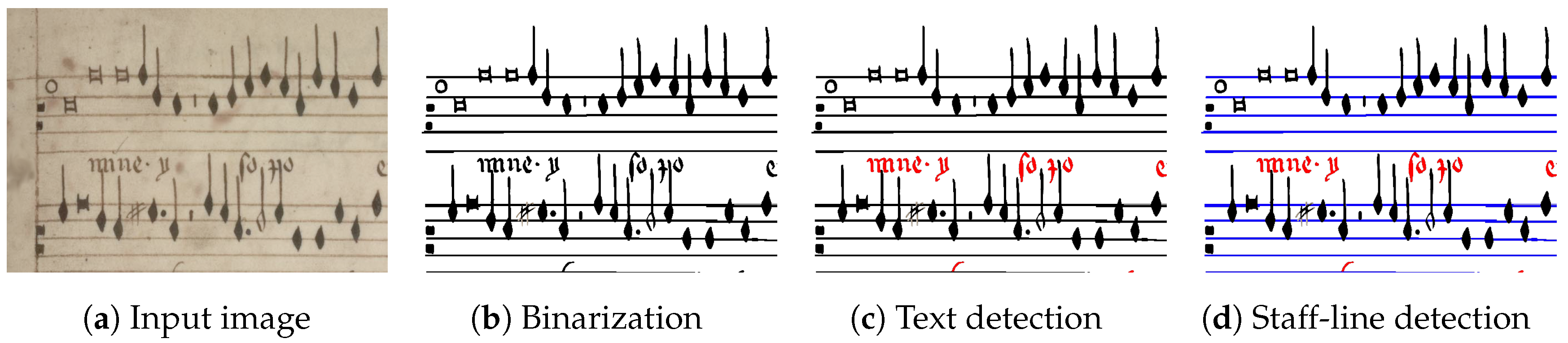
Although rarely formulated in this way, the document processing of music score images can be seen as a pixel-level problem. For instance, for the input image depicted in Figure 2a, we want to know whether each pixel belongs to the foreground or to the background (Figure 2b). This corresponds to the document image binarization step, from which the background layer is ignored. Hence, those classified as foreground are further categorized into text or music elements, because they shall be processed by different automatic algorithms (Figure 2c). In the latter case, we want to know whether a pixel belongs to a staff line or not, as this information is valuable for several reasons such as the segmentation of single notes as well as determining the pitch (Figure 2d). In the framework described in this paper, we propose to tackle all these processes in a single step.
The document processing can be reformulated as a supervised classification task in which a model is trained to distinguish the category to which every pixel belongs. Formally, our approach considers a model that categorizes a given pixel into four possible classes: background, text, staff line, and symbol. Although we instantiate our approach to this specific label set, the framework is rather general and can be used for any number of categories.
In our framework, this classification process is carried out by means of Deep Learning. Recently, Deep Neural Networks (DNN) have shown a remarkable leap of performance in pattern recognition. Specifically, CNN have been applied with great success for the detection, segmentation, and recognition of objects and regions in images, approaching human performance on some of these tasks [7].
CNN are composed of a series of filters (i.e., convolutions) that obtain several intermediate representations of the input image. These filters are applied in a hierarchy of layers, each of which represent different levels of abstraction; while filters of the first layers may enhance details of the image, filters of the last layers may detect high-level entities [6]. The key to this approach is that, instead of being fixed, these filters are modified through a gradient descent optimization algorithm called backpropagation [39].
One of the main advantages of CNN is its ability to learn the representation that is needed for the classification task without any human intervention, achieving greater generalization and adaptability when applied to different manuscripts. In other words, these networks learn a suitable representation from raw data, without the need of performing a feature extraction process. Since collections of music documents are a rich source of highly complex information—often more heterogeneous than other types of documents—a framework based on CNN is promising.
Implementation Details
With our method, a classifier was trained to differentiate pixels belonging to different categories. To analyze the organization of musical documents, we hypothesized that a pixel can be correctly classified by using neighboring information. In other words, we assumed that the surrounding region of a pixel contains enough discriminative information to classify it into a class. For example, whereas zones in the image with staff lines usually indicate sectors where music notation is present, areas without staff may indicate other type of content. Our approach, therefore, exploits these local features to correctly distinguish the categories of the different elements within a musical document.
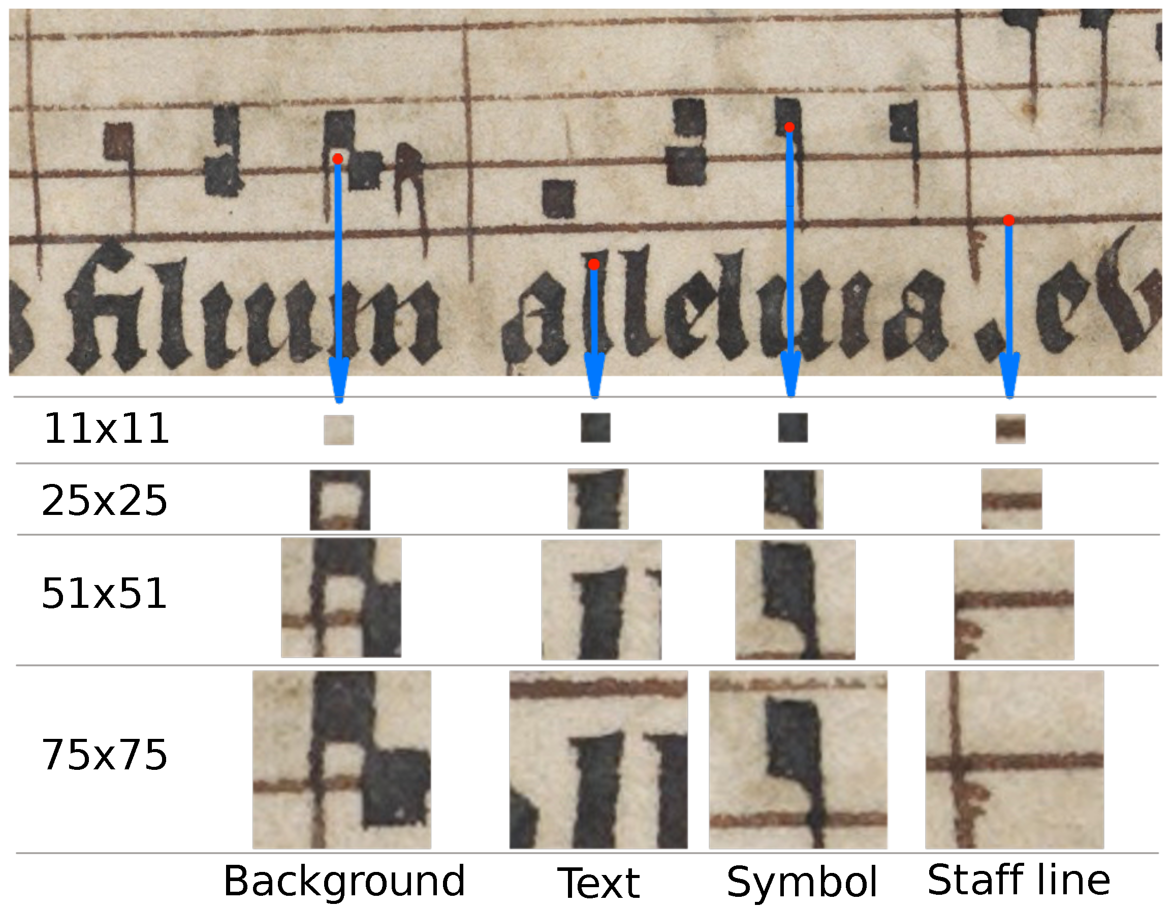
In our framework, the input to the CNN is a rectangular patch of the input image centered at the pixel of interest. In principle, the size of this block should be determined according to the scale of the documents and the content in them, since they affect the information that is retrieved in such portion. As an illustrative example, we can see in Figure 3 the neighborhood of some pixels of interest, with different window sizes. It can be observed that the choice of the block size establishes a trade-off between localization and representativeness: in the smallest blocks, the neighborhood might provide insufficient information but the pixel of interest is well located; on the other hand, larger blocks have much more information to discriminate but it is more complicated to know which pixel in particular is being classified. In fact, large portions from near pixels will depict very similar blocks.
If the CNN has been properly trained to classify blocks into one of the considered categories, it can be used to perform the document processing of a music score image. To do so, each pixel of the image is queried, and its feature block is forwarded and processed by the network, as illustrated in Figure 4. As a result of this process, a probability is obtained for each category, and then we label that pixel according to the category that retrieves the highest probability.
Concerning the CNN configuration, it is still an open question what hyper-parameters (e.g., number of layers, number of filters per layer, size of the filters, etc.) are useful to a greater or lesser extent for this task. This is why we carried out a thorough study of different CNN configurations. The idea is not to find an optimal configuration, which would be unfeasible to demonstrate, but to study what hyper-parameter configurations make a greater difference in performance and computational cost, as well as to analyze the best level of accuracy that can be attained using this approach.
Regardless of the specific configuration, the training stage is based on pairs of images depicting original sources with their corresponding human-labeled ground-truth image, as illustrated in Figure 5. Thus, the creation of the training set consists in extracting the blocks of each pixel from the original source, indicating the category given by the pixel at issue in the ground-truth image.
The learning process is carried out by means of stochastic gradient descent [40], which modifies the CNN parameters through backpropagation to minimize the cross-entropy loss function. Let and be the set of training samples and the set of categories of the problem, respectively. Let us denote the prediction of the network for input x being the category c as , while its desired activation is denoted by . Given that the network is used for classification, the desired activation is 1 if c is the actual category of input x, and 0 otherwise. Then, the loss L for X can be computed as:
This loss function is designed for tasks in which the number of samples is balanced. As mentioned previously, this is not the case in music score images. However, this problem can be easily solved during training by simply restricting ourselves to consider the same number of samples from each class in the training set.
4. Experimental Setup
Recalling from above, the paper presents a purely experimental study of the capabilities that a CNN can offer for the document processing of music score images. Before moving on to the different configurations and their results, we introduce below the corpora, the evaluation metrics, and the evaluation methodology considered.
4.1. Corpora
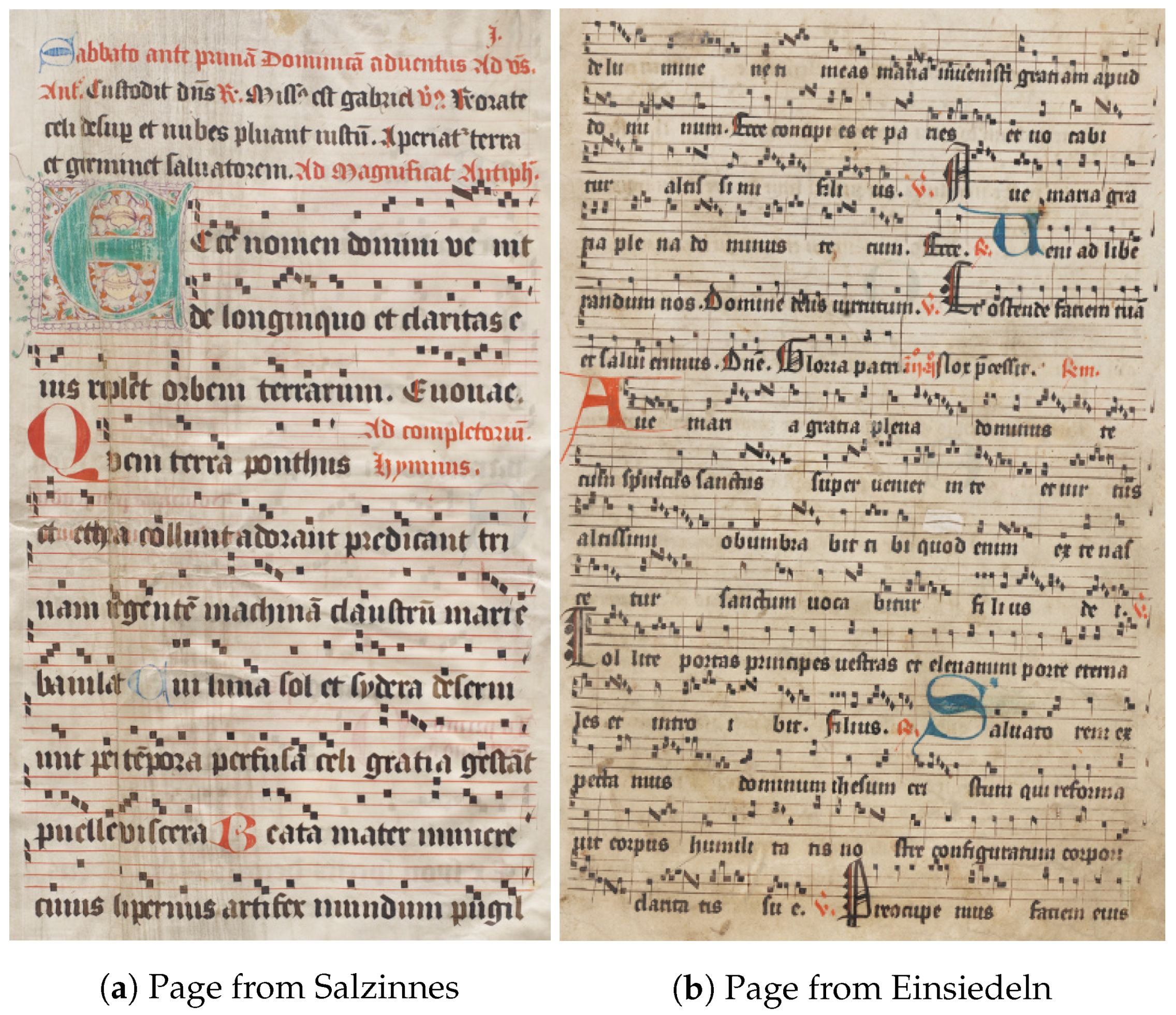
For the evaluation of the approach, we make use of high-resolution image scans from two different old music manuscripts. The first corpus is a subset of 10 pages of the Salzinnes Antiphonal (CDM-Hsmu 2149.14) (see https://cantus.simssa.ca/manuscript/133/), which is dated 1554–1555. The second corpus consists of 10 pages of the Einsiedeln, Stiftsbibliothek, Codex 611(89), from 1314 (see http://www.e-codices.unifr.ch/en/sbe/0611/). Example pages from these corpora are shown in Figure 6a,b, respectively. The image scans of these two manuscripts have zones with different lighting conditions, which may have affected the performance of the models that were evaluated. Einsiedeln manuscript scans, in particular, present areas with severe bleed-through that may mislead the learned model. The images were used with their original codification (RGB) with no pre-processing, given that CNN is designed to deal with the original data.
Table 1 gives an overview of the two corpora considered here with some specific features. As can be observed, the distribution of pixels into the considered categories is highly biased: the background is the most represented category by a wide margin. Therefore, we clearly face a classification problem with imbalanced data.
The ground-truth data from the corpora was created by manually labeling pixels into the four categories mentioned above. This human labor may take time, and therefore it is interesting to study the capacity of the CNN to make the most out of the available data.
4.2. Evaluation Metrics
Given the distribution of data in terms of the different categories, we shall consider appropriate metrics for such imbalanced datasets. For instance, the F-measure () typically represents a fair metric in these scenarios. In a two-class classification problem, this measure can be computed as
where True Positive (TP) stands for the correctly classified elements of the majority class, False Positive (FP) represents the misclassified elements from the majority class, and False Negative (FN) stands for the misclassified elements of the minority class.
To compute a single metric encompassing all possible classes, can be reformulated into two types of averages: macro and micro averages (F and F, respectively); both averages are typically applied in multi-class data-imbalance classification tasks [41]. The difference between the two versions is that F is obtained from the sum of all class-wise TP, FP, and FN, and the subsequent application of Equation (2), whereas F is computed as the average of all class-wise . That is:
where N is the number of categories.
These evaluation metrics can be complemented with precision (P) and recall (R) figures of merit:
These metrics are interesting when we want to focus on a single category (the positive one): P measures the certainty with regard to a sample classified as positive, whereas R estimates the possibility of missing a positive sample.
The metrics stated above are widely applied to classification problems when the relevance of each sample is not significant. In our context, the samples can vary in relevance according to their location within the document itself. Thus, samples that are at the edge of two categories—for example, background and staff line—are less relevant as long as they are categorized as one of these categories. This may lead to thinner or thicker elements, which is unlikely to affect the remaining stages of the OMR system. On the other hand, it may severely affect the evaluation metrics.
Therefore, we considered a novel metric to evaluate the performance of the models taking into account this issue. This new metric evaluates a pixel and compares the result of its classification with the actual category of adjacent neighbors—vertical and horizontal. If the prediction of the CNN matches either the actual category of the pixel or that of any adjacent pixel, it is considered as a pseudo-TP. Consequently, all metrics computed with pseudo-TP are named with the pseudo prefix. Note that ground-truth data is often subjective, especially for border pixels, and therefore these metrics may be more convenient.
Finally, given that, in a real scenario, the CNN must evaluate many pixels, we also considered the computational cost of the classification process. Specifically, we considered the number of pixels that can be processed per second as a measure of computational cost. The training process is not considered within this cost because it can be done asynchronously, before actually using the classification process.
All the experiments were performed in similar conditions on a general-purpose computer with the following technical specifications: Intel(R) Core(TM) i7-7700HQ CPU @2.8GHz, 32GB RAM, GTX1070 GPU and Linux Mint 18.2 (64 bits) operating system. The code was written using Python language (v2.7) and Keras framework. The classification step was carried out considering batches of 64 samples for boosting the performance.
4.3. Evaluation Methodology
The large number of pixels to process—with around 20,000,000 pixels per page—clearly represents an obstacle to perform a comprehensive experimentation. This is why we must consider a strategy to reduce the cost of the evaluation process.
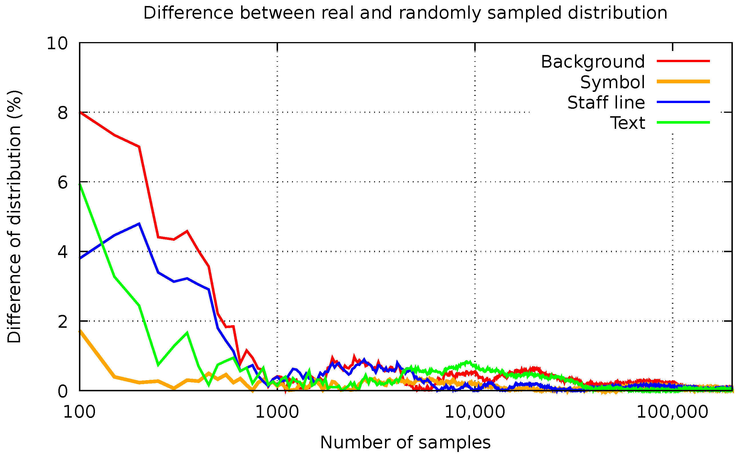
The idea is that we did not process documents entirely to compute the evaluation metrics, but a reduced subset of pixels. The number of samples to process, however, must be large enough so that the results can be considered reliable, especially in regard to the distribution of pixels per category (see Table 1). Consequently, we performed a preliminary study in which pixels of the documents were extracted randomly, and organized them according to the category to which they belong. In Figure 7, we show the difference between the distribution of pixels of each category that we found in this random subset and their actual distribution (y-axis), with respect to how many pixels were randomly extracted (x-axis). It can be observed that the curve stabilizes quickly, and so 100,000 random samples are enough to attain a difference between both distributions below in all categories. Therefore, the evaluation of the classification process considering a random subset of 100,000 pixels can be considered reliable enough for our experimental study.
Nevertheless, to provide a more robust set of evaluation metrics, a five-fold cross-validation partitioning was implemented. At each experiment with one corpus, one fold consisting of two pages—not necessarily consecutive ones—was used as test set from which those 100,000 random samples are extracted. The remaining 8 pages were used for building the training set.
5. Experiments
We present in this section the series of experiments for the thorough evaluation of the CNN approach for document processing of music score images. The experimentation was divided into several parts. The results reported in Section 5.1 focus on measuring the performance variability as regards some of the most critical parameters related to CNN. The best models obtained from these experiments are evaluated and analyzed in Section 5.2. Finally, in Section 5.3, we evaluate the capabilities of these models for manuscript adaptation—a concept that refers here to using a trained model to solve the task in a different, albeit similar, manuscript.
5.1. CNN Parameterization
The specific configuration of a CNN comprises several hyper-parameters that must be fixed according to the task at issue. Our intention is to assess how modifications in the most relevant hyper-parameters affect the performance of the classification process. To reduce the complexity of these experiments, however, we restricted ourselves to considering only the Einsiedeln corpus, which, as shown below, is the most challenging one—and F as a summary of the accuracy.
One of the relevant parameters is the size of the input layer; that is, the size of the block used as input. There is no input size that will work for all manuscripts, as its goodness depends on unpredictable factors such as the resolution and size of the images. That is why we conducted experiments in this regard. Note that the spacing between staff lines in the corpora was provided (Table 1), which is a typical scale reference in OMR, and can be used to generalize the results of our experiments. We evaluated rectangular portions with different widths and heights, always with the pixel to classify in the center of them. The depth of the network (number of layers) is another parameter that must be adjusted. To standardize the experiments, let us assume that a layer always consists of a variable number of stacked convolutions with Batch Normalization [42] and Rectified Linear Unit (ReLU) activation [43] followed by a down-sampling operator. The down-sampling operation is implemented here as a max-pooling operation. Figure 8 shows examples of layers with variable number of stacked convolutions (1–3). The hyper-parameters of the convolution operators, namely number of filters and kernel size, were also evaluated. The final set of parameters is listed in Table 2.
Since the possible combinations of all the different parameters lead to a huge set of different neural networks to be trained per fold, we propose a serialization of the experiments. That is, we first fixed some values and varied the parameters that seem most relevant: squared input block sizes, depth of the network, and convolutions per layer. Following this strategy, we reduced the number of configurations of the first experiment to only 171. Then, the rest of the parameters were introduced, namely the number of filters per convolution and the kernel size of the convolutions. In addition, we considered non-squared input sizes.
Although the number of training samples may affect the performance of the network, its relevance is measured separately. Until stated otherwise, the training set consisted of 20,000 random samples from each class. This way we ensured that the number of samples of each categories in the training process is equal, which avoids biasing the model towards any of the categories.
5.1.1. Input Size, Depth, and Convolutions Per Layer
We report in Table 3 the first experimental results, varying the squared input block sizes, depth of the network, and convolutions per layer. The resulting configurations fixed the number of filters per convolution to 32, the size of the kernel to , and the number of random samples of each category to 20,000. In addition to the accuracy (in terms of F), we measured the ability of the model to process pixels per second.
The first thing to remark is that, indeed, the parameters considered here do affect the accuracy the CNNs attained. For instance, there is a spread of values between the figures of F of up to 20% (from 66.7% to 86.9%). In general, some tendency towards improvement can be seen with the highest image sizes and depths of the network, where the number of convolutions per layer is somewhat less relevant. The behavior of different combinations of hyper-parameters is not easily predictable, however, since the set of best solutions (86.9% of F) consists of rather heterogeneous configurations. On the contrary, the computation time follows a much clearer trend: the greater the number of input pixels and the number of convolutions per layer, the fewer the number of pixels that are processed per second.
Given that there are several equally-optimal solutions as regards accuracy, we selected the one with the best efficiency as representative for the next experiments: input blocks, five layers, and one convolution operation per layer.
5.1.2. Number of Filters, Kernel Size, and Non-Squared Input
According to the results in the previous section, we fixed the base CNN to five layers, and one convolution operation per layer. We now evaluate the performance with different number of filters per convolution and different kernel sizes. In addition, we consider non-squared input sizes, restricting any of the dimensions to 51. The results of this experiment are reported in Table 4.
The results confirm that these parameters have a less influence than the previous ones on the accuracy, although their relevance is still high for the computation time. Initially, the base CNN improved by adding more filters—to some extent—while the best results maintained smaller kernel sizes. The upward trend of the computational cost is also clear with respect to increasing the number of filters and the size of the kernel, suggesting a much stronger influence on the part of the former.
It is also appreciated that considering non-squared image sizes can be beneficial, as the results vary considerably in this regard. This fact is not accidental, as the relevant information to distinguish the category of a pixel is usually found on the horizontal (for example, in the case of text) or the vertical (for example, to find the staff lines) axes of such pixel, so the information of the diagonal neighborhoods is less relevant.
The best result in terms of accuracy is obtained when 256 filters per convolution are established, with a kernel size of , and input blocks of (height and width, respectively). This configuration improves the accuracy of the base CNN up 1%, from 86.9% to 88.0%. In our experiments, this neural configuration classified 900 pixels per second, on average. In the manuscripts considered (Table 1), this represents a cost of around 6 h to completely classify a whole page.
Throughout these experiments, however, we did not make any comments about the time it takes for each model to train. The training time depends on multiple factors such as the convergence of the model, the size of the training set, the network model, and the underlying hardware. In our experiments, the training time ranged from half an hour, for the simplest cases, up to 10 h, being the size of the input patch the most relevant factor in this regard. Although the training time may become important in some scenarios because it imposes restrictions on parameter optimization and evaluation, in this article, we are more concerned about the network topology and the parameter values that allow to achieve the best accuracy in our corpora.
5.1.3. Training Set Size
Finally, the relevance of the training set size in regard to the CNN performance is presented below. Starting with a reduced training set size, we incrementally increased the size of that training set to measure the amount of data that the selected model needs to solve the task successfully.
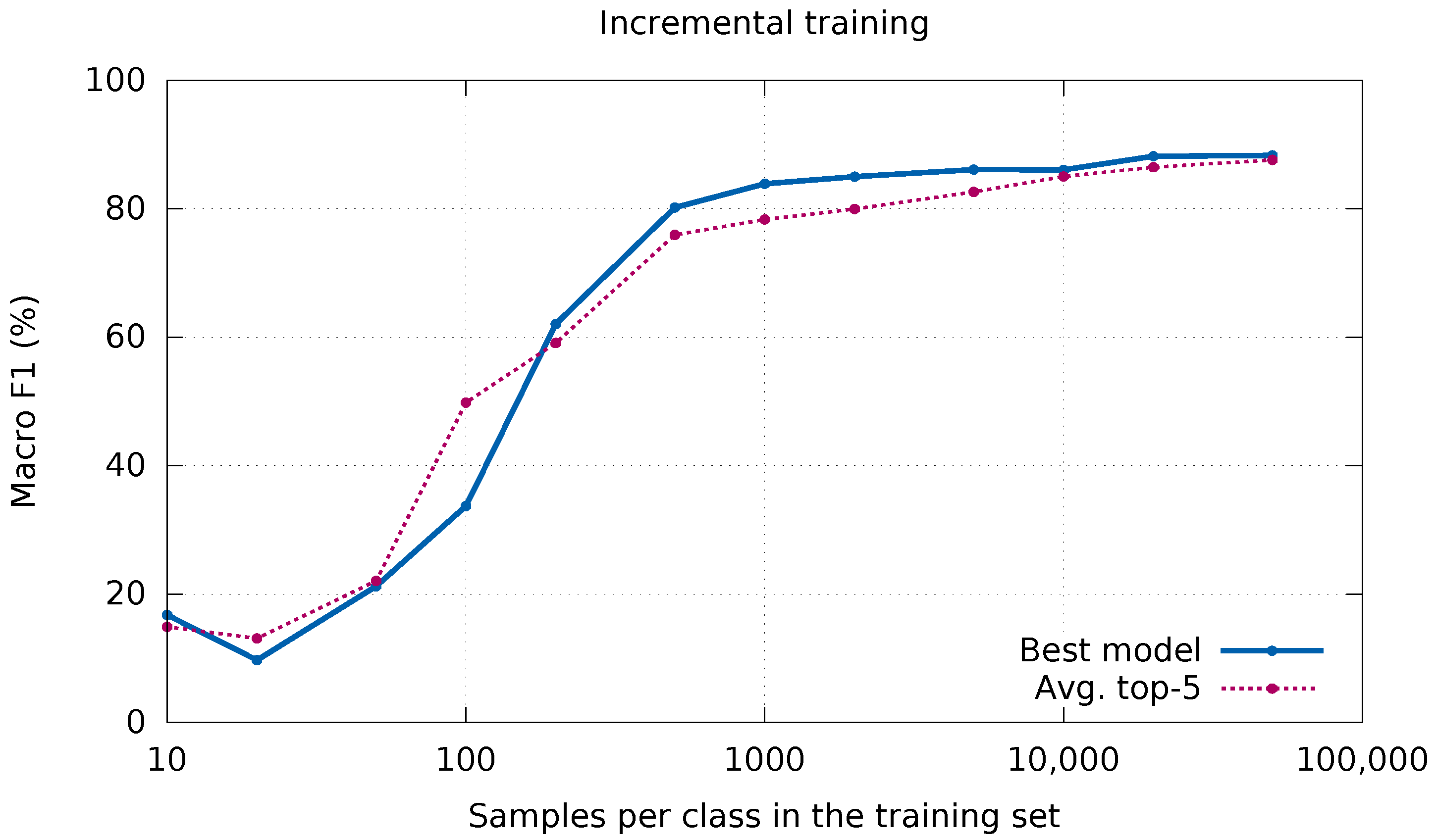
Figure 9 shows the performance curve. Note that, for the sake of visualization, the graphic does not use a linear x-axis. In addition to the curve obtained by the selected network (plain blue line), the average of the five best configurations in Table 4 is also added to draw more general conclusions. Some confusing results are observed for the smallest training set sizes. However, given the limited number of samples per class, they can be considered negligible. Afterwards, the curve is stabilized from 1000 samples per class, obtaining residual improvements by further increasing the size of the training set.
Figure 9 also shows that the selected CNN reaches a fair performance with few samples: from 500 samples, results are already above 80%, while from 5000 the results are less than 2% below the final accuracy. On average, the behavior is quite similar—yet slightly lower—so it can be assumed that this is a rather general trend. As a positive conclusion, the CNN does not need an inordinate amount of data to obtain results that can be useful in practice. Note that each pixel of an image represents a sample, so labeling a relatively small portion of an image provides a large training set.
5.2. Detailed Results
In this section, we analyze in detail the performance that was attained using the best CNN configuration of the previous section as shown in Table 4. Specifically, the network configuration finally considered consists of five layers, each of which contains one convolution operator composed of 256 filters of size . It accepts input blocks. In addition, the network was trained with 50,000 samples of each class. Results of this model taking into account all the metrics previously described over the two corpora considered are reported in Table 5.
According to these figures, we can observe that the results vary visibly between the two corpora. While results are closer to the optimum in Salzinnes, the CNN finds more difficulties in Einsiedeln. In general, however, we can consider that the performance is reasonable to cope with the document processing task in practice, given that actual metrics (F and F) are around 90% in all cases.
Concerning specific categories, it can be observed that the results follow similar trends in both corpora: the background pixels are quite well estimated, whereas a lower accuracy is obtained in the other categories—particularly, is remarkably below average results, as well as in Salzinnes. In general, the P metric is slightly worse than R, which means that the CNN misses few elements of each category but produces noisy pixels.
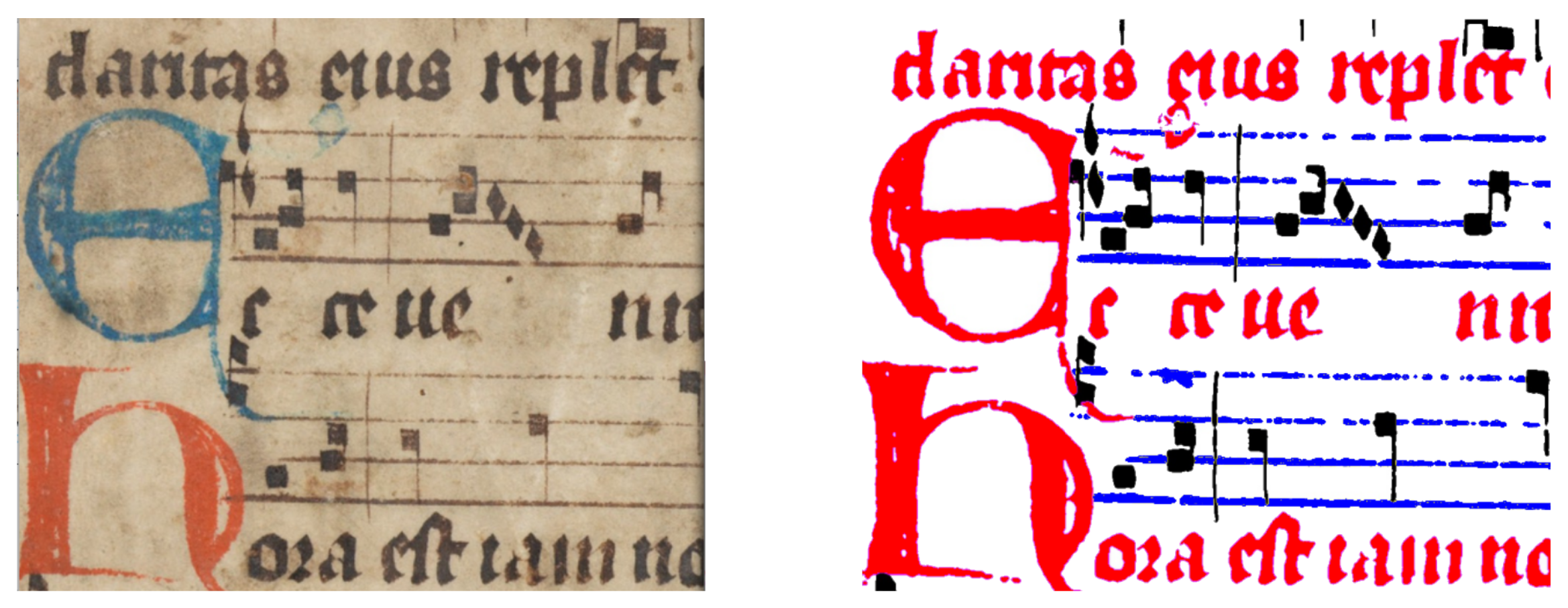
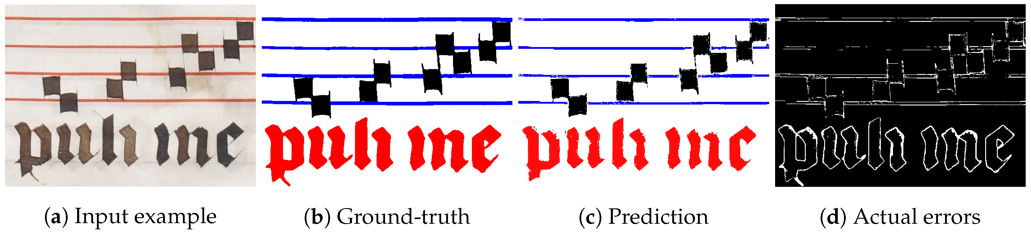
As regards the pseudo-metrics introduced above, it is obvious that these lead to significantly better results. That is to say, the hypothesis that many errors occur near the borders between symbols is verified; otherwise, the pseudo-metrics would not have increased noticeably. As an example of this phenomenon, Figure 10 shows a qualitative example from Salzinnes manuscripts. It depicts the difference between the CNN prediction and the human-labeled ground-truth data, highlighting the areas where there are discrepancies (see Figure 10d).
It can be clearly observed that many of the errors are found around the edges, obtaining thinner elements in the prediction. Although it seems that this especially affects the text elements, note that the boundaries of the characters represent a small percentage of their pixels. However, the edge of the staff lines represents a higher percentage of their area, for which the difference between actual and pseudo metrics is more relevant ().
This phenomenon should not severely affect the quality of the document processing and, therefore, it can be considered that the pseudo-metrics report values closer to performance in practice. In addition, the labeling of ground-truth is subjective, which further justifies the use of these pseudo-metrics.
Finally, we evaluated classic schemes for the different stages of document processing in musical score images, in order to compare their performance with the CNN-based approach. The evaluation was based on the comparison made in previous work for the binarization and staff-line removal stages [8], but adding here the detection of lyrics as well. The set of heuristic strategies to segment the images into the considered categories consists of: the document binarization algorithm proposed by Wolf et al. [44], the Stable Paths algorithm for staff-line removal [21], and the algorithm proposed by Burgoyne et al. [30] to extract lyrics. To actually obtain the four categories considered, we assumed that background are those pixels removed by the binarization algorithm and text corresponds to pixels belonging to the elements detected during lyrics extraction. From the remaining pixels, staff line are those removed by the staff-line removal algorithm, while the rest are thus considered as belonging to the note category.
Table 6 shows the comparison in terms of F (actual and pseudo) between our CNN and the aforementioned strategies. In general, trends are similar (higher accuracy in Salzinnes than in Einsiedeln, and higher figures of pseudo F than actual F). However, it can be observed that the CNN approach is clearly superior to the set of classical strategies. Thus, in Einsiedeln, the CNN improves up to 8% the set of classical strategies (actual F), while in Salzinnes the improvement is around 4% in both metrics.
The objective of studying a machine learning approach for document processing of music score images is to provide a general framework that can be applied to different manuscripts. Nevertheless, we empirically demonstrated that it leads to substantial improvements in classification accuracy at pixel level in comparison with classical algorithms.
5.3. Cross-Manuscript Adaptation
We also studied how CNN models behave when analyzing a different manuscript from that of the training set. The idea is to give some insights on how to take advantage of the knowledge acquired by the CNN when a new type of manuscript is to be processed. Ideally, it would not be necessary to have new ground-truth data when working with similar music manuscripts, thus we wanted to assess whether starting from a pre-trained network reduces the amount of new labeled data; that is, if we can train the CNN in an incremental learning fashion. In such a case, it would help to reduce the initial effort in dealing with a new manuscript.
First, we check how the CNN behaves when it is directly used to process another manuscript, without any new information. In particular, we measured the performance obtained by the network trained for Einsiedeln over Salzinnes, and vice versa. Table 7 summarizes the performance comparison of this experiment. For simplicity, the performance is only presented in terms of actual F.
The most interesting conclusion that can be drawn from these figures is that the cross-manuscript adaptation is actually feasible. Thus, training in Einsiedeln attains results in Salzinnes that are close to those obtained with its own model. The difference is only 6% (from 93.4% to 87.2%). Furthermore, it is observed that the network trained in Salzinnes obtains fair results when analyzing the Einsiedeln manuscript, while producing some accuracy loss with respect to the network trained specifically for it (from 88.6% to 73.3%).
Although the networks do not guarantee the same accuracy on different manuscripts, using a pre-trained network involves a great improvement with respect to training a network anew. In fact, if we compare the results of the initial performance between the cross-manuscript adaptation experiment shown in Table 7 with the evolution of the learning process in regard to the size of the training set in Figure 9, we can see that the adapted model outperforms all training set sizes with less than the optimal minimum value that reported a fair performance, with 500 samples per class.
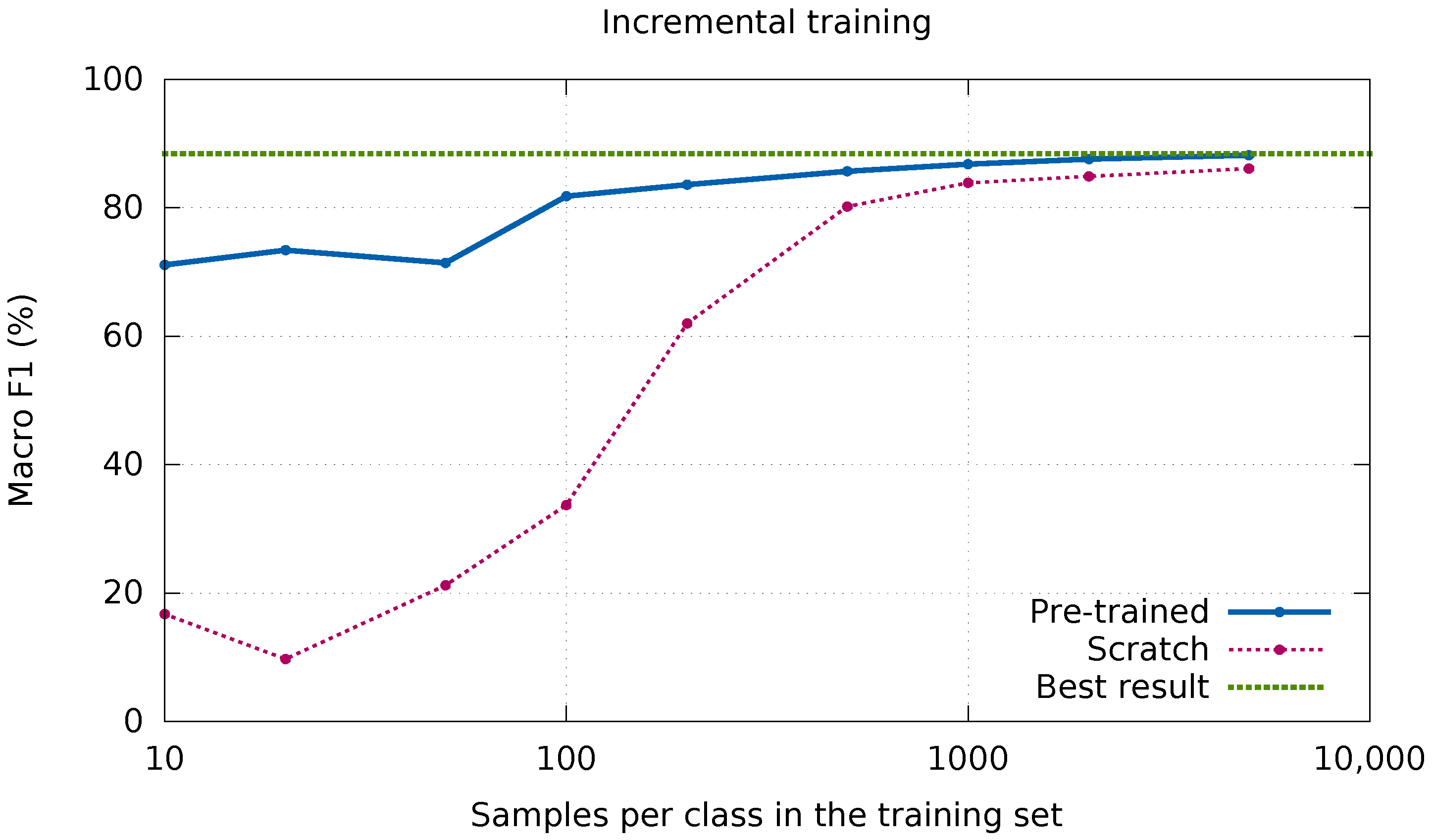
Thus, as the last experimental analysis, we wanted to certify that starting from a pre-trained network will bear a lesser need of new labeled data. We show in Figure 11 the F curves obtained for an incremental training set size, depicting the evolution curves of starting from a pre-trained network and starting from scratch (taken from Figure 9). In addition, we have indicated the best result obtained with manuscript-specific data.
It can be seen that the CNN approaches the optimum much faster when it starts with prior knowledge. This comes as no surprise as we know that it already attained a fair result before providing it with new data. Furthermore, it is observed that modest improvements can be obtained by providing more than 1000 samples per class. In the case the network is pre-trained, it achieves results above 80% with only 100 samples of each class. In contrast, when training a network from scratch, that amount of samples leads to very poor results (less than 40% of F), and more than 500 samples of each class are needed to reach a similar performance.
The main conclusion drawn from this cross-manuscript adaptation experiment is that the CNNs are able to transfer knowledge across manuscript types. In some cases it might not be necessary to retrain the models, as happens here for classifying the Salzinnes manuscript, with a model trained for Einsiedeln. Additionally, the convergence towards a good performance is much faster, thereby needing fewer manuscript-specific training data. As a result, according to our experiments, starting from a pre-trained network is profitable in any situation.
6. Conclusions
In this work, we studied exhaustively the use of CNN to perform the task of document processing in musical score images. Specifically, the task was posed as a problem of classification at pixel level: each pixel must be categorized by the model from its contextual graphic information into background, note, text, or staff line. The advantage of this approach is twofold. On the one hand, it allows to perform the complete process in a single step. On the other hand, being a machine learning approach, it is generalizable to any type of score as long as training data is available. The main objective of this work was to conduct an experimental study of the capabilities offered by this approach in various aspects.
In the first experiment, the performance of CNNs was measured according to their configuration, and parameters such as the size of the input, the depth of the network, or the configuration of the convolutions were analyzed. It was established that some parameters, such as the size of the input block or the depth of the CNN, have a larger impact on the performance, while other parameters, such as the number of filters per convolution or the kernel size, affect the performance to a lesser extent. In addition, the computation time varies considerably amongst the different configurations, so that if this parameter is relevant in practice, it would be necessary to consider configurations with a better trade-off between effectiveness and efficiency. Furthermore, it has been observed that the models do not need a large number of training samples to produce good results.
In addition, we analyzed the performance limit that can be achieved by tuning the CNN. The results showed that a limit of around 90% is achieved in the general cases with a good CNN tuning. A more in-depth analysis with the proposed pseudo-metrics, in which the pixels over the edges between symbols are treated in a particular way, reflects that the tuning approaches the optimum in the practical sense.
Finally, a cross-manuscript adaptation experiment was carried out, in which the CNN were evaluated in a different type of manuscript than the one with which they have been trained. The results indicate that this approach of starting from a pre-trained network is very effective, requiring much less training data for the new manuscript.
Although it was shown that the margin for improvement as regards to accuracy is rather limited, there are other issues on which this line of research can be extended. For instance, it has been observed that the approach of document processing presented in this paper involves a high computational time. Since OMR—especially for ancient manuscripts—is a process that is not necessarily intended to be performed in real time, this cost could be detrimental in an interactive scenario in which user and machines collaborate to solve the task together [45]. Therefore, a research path aiming at accelerating the processing of complete documents without losing classification quality is of interest. In this regard, our idea is to replace the current model, which performs an independent classification for each pixel of the image, by a model able to classify complete patches of the image.
Furthermore, it would be interesting to study schemes that allow a greater adaptability of the networks. To this end, specific semi-supervised learning algorithms could be used, in which the networks learn to adapt to a new manuscript by just providing them with new (unlabeled) images. This can be performed by promoting convolutional filters that are both useful for the classification task and invariant with respect to the difference between manuscript types [46].
Author Contributions
J.C.-Z. and F.J.C. conceived and designed the experiments; F.J.C. performed the experiments; J.C.-Z., F.J.C., G.V. and I.F. analyzed the data; G.V. and I.F. contributed material and tools; and J.C.-Z. and F.J.C. wrote the paper, with substantial contributions from G.V. and I.F.
Acknowledgments
This work was supported by the Social Sciences and Humanities Research Council of Canada, and Universidad de Alicante through grant GRE-16-04.
Conflicts of Interest
The authors declare no conflict of interest. The founding sponsors had no role in the design of the study; in the collection, analyses, or interpretation of data; in the writing of the manuscript, and in the decision to publish the results.
Abbreviations
The following abbreviations are used in this manuscript:
| OMR | Optical Music Recognition |
| CNN | Convolutional Neural Network |
| OCR | Optical Character Recognition |
| DNN | Deep Neural Networks |
| HMM | Hidden Markov Models |
| FCNN | Fully-Convolutional Neural Network |
| P | Precision |
| R | Recall |
| TP | True Positive |
| FP | False Positive |
| FN | False Negative |
References
- Bainbridge, D.; Bell, T. The challenge of optical music recognition. Comput. Hum. 2001, 35, 95–121. [Google Scholar] [CrossRef]
- Byrd, D.; Simonsen, J.G. Towards a standard testbed for optical music recognition: Definitions, metrics, and page images. J. New Music Res. 2015, 44, 169–195. [Google Scholar] [CrossRef]
- Duda, R.O.; Hart, P.E.; Stork, D.G. Pattern Classification, 2nd ed.; John Wiley & Sons: New York, NY, USA, 2001. [Google Scholar]
- O’Gorman, L.; Kasturi, R. Document Image Analysis; IEEE Computer Society Press: Washington, DC, USA, 1995. [Google Scholar]
- Doermann, D.; Tombre, K. Handbook of Document Image Processing and Recognition; Springer: London, UK, 2014. [Google Scholar]
- Krizhevsky, A.; Sutskever, I.; Hinton, G.E. Imagenet classification with deep convolutional neural networks. In Proceedings of the 26th Annual Conference on Neural Information Processing Systems, Lake Tahoe, NV, USA, 3–6 December 2012; pp. 1106–1114. [Google Scholar]
- LeCun, Y.; Bengio, Y.; Hinton, G. Deep learning. Nature 2015, 521, 436–444. [Google Scholar] [CrossRef] [PubMed]
- Calvo-Zaragoza, J.; Vigliensoni, G.; Fujinaga, I. One-step detection of background, staff lines, and symbols in medieval music manuscripts with convolutional neural networks. In Proceedings of the 18th International Society for Music Information Retrieval Conference (ISMIR), Suzhou, China, 23–27 October 2017; pp. 724–730. [Google Scholar]
- Rebelo, A.; Fujinaga, I.; Paszkiewicz, F.; Marçal, A.R.S.; Guedes, C.; Cardoso, J.S. Optical music recognition: State-of-the-art and open issues. Int. J. Multimed. Inf. Retr. 2012, 1, 173–190. [Google Scholar] [CrossRef]
- Louloudis, G.; Gatos, B.; Pratikakis, I.; Halatsis, C. Text line detection in handwritten documents. Pattern Recognit. 2008, 41, 3758–3772. [Google Scholar] [CrossRef]
- He, S.; Wiering, M.; Schomaker, L. Junction detection in handwritten documents and its application to writer identification. Pattern Recognit. 2015, 48, 4036–4048. [Google Scholar] [CrossRef]
- Giotis, A.P.; Sfikas, G.; Gatos, B.; Nikou, C. A survey of document image word spotting techniques. Pattern Recognit. 2017, 68, 310–332. [Google Scholar] [CrossRef]
- Sauvola, J.; Pietikäinen, M. Adaptive document image binarization. Pattern Recognit. 2000, 33, 225–236. [Google Scholar] [CrossRef]
- Gatos, B.; Pratikakis, I.; Perantonis, S.J. Adaptive degraded document image binarization. Pattern Recognit. 2006, 39, 317–327. [Google Scholar] [CrossRef]
- Howe, N.R. Document binarization with automatic parameter tuning. Int. J. Doc. Anal. Recognit. (IJDAR) 2013, 16, 247–258. [Google Scholar] [CrossRef]
- Pinto, T.; Rebelo, A.; Giraldi, G.; Cardoso, J.S. Music score binarization based on domain knowledge. In Pattern Recognition and Image Analysis: 5th Iberian Conference (IbPRIA); Vitrià, J., Sanches, J.M., Hernández, M., Eds.; Springer: Berlin/Heidelberg, Germany, 2011; pp. 700–708. [Google Scholar]
- Vo, Q.N.; Kim, S.H.; Yang, H.J.; Lee, G. An MRF model for binarization of music scores with complex background. Pattern Recognit. Lett. 2016, 69, 88–95. [Google Scholar] [CrossRef]
- Burgoyne, J.A.; Pugin, L.; Eustace, G.; Fujinaga, I. A comparative survey of image binarisation algorithms for optical recognition on degraded musical sources. In Proceedings of the 8th International Conference on Music Information Retrieval (ISMIR), Vienna, Austria, 23–27 September 2007; pp. 509–512. [Google Scholar]
- Calvo-Zaragoza, J.; Gallego, A. A Selectional Auto-Encoder Approach for Document Image Binarization. arXiv, 2017; arXiv:1706.10241. Available online: https://arxiv.org/abs/1706.10241(accessed on 24 April 2018).
- Dalitz, C.; Droettboom, M.; Pranzas, B.; Fujinaga, I. A comparative study of staff removal algorithms. IEEE Trans. Pattern Anal. Mach. Intell. 2008, 30, 753–766. [Google Scholar] [CrossRef] [PubMed]
- Dos Santos Cardoso, J.; Capela, A.; Rebelo, A.; Guedes, C.; Pinto da Costa, J. Staff detection with stable paths. IEEE Trans. Pattern Anal. Mach. Intell. 2009, 31, 1134–1139. [Google Scholar] [CrossRef] [PubMed]
- Rebelo, A.; Cardoso, J. Staff line detection and removal in the grayscale domain. In Proceedings of the 12th International Conference on Document Analysis and Recognition (ICDAR), Washington, DC, USA, 25–28 August 2013; pp. 57–61. [Google Scholar]
- Dutta, A.; Pal, U.; Fornés, A.; Lladós, J. An efficient staff removal approach from printed musical documents. In Proceedings of the 2010 20th International Conference on Pattern Recognition (ICPR), Istanbul, Turkey, 23–26 August 2010; pp. 1965–1968. [Google Scholar]
- Su, B.; Lu, S.; Pal, U.; Tan, C. An effective staff detection and removal technique for musical documents. In Proceedings of the 2012 10th IAPR International Workshop on Document Analysis Systems (DAS), Gold Cost, Australia, 27–29 March 2012; pp. 160–164. [Google Scholar]
- Géraud, T. A morphological method for music score staff removal. In Proceedings of the 2014 IEEE International Conference on Image Processing (ICIP), Paris, France, 27–30 October 2014; IEEE: Piscataway, NJ, USA, 2014; pp. 2599–2603. [Google Scholar]
- Montagner, I.D.S.; Hirata, N.S.T.; Hirata, R. Staff removal using image operator learning. Pattern Recognit. 2017, 63, 310–320. [Google Scholar] [CrossRef]
- Calvo-Zaragoza, J.; Micó, L.; Oncina, J. Music staff removal with supervised pixel classification. Int. J. Doc. Anal. Recognit. 2016, 19, 211–219. [Google Scholar] [CrossRef]
- Calvo-Zaragoza, J.; Pertusa, A.; Oncina, J. Staff-line detection and removal using a convolutional neural network. Mach. Vis. Appl. 2017, 28, 665–674. [Google Scholar] [CrossRef]
- Gallego, A.; Calvo-Zaragoza, J. Staff-line removal with selectional auto-encoders. Expert Syst. Appl. 2017, 89, 138–148. [Google Scholar] [CrossRef]
- Burgoyne, J.A.; Ouyang, Y.; Himmelman, T.; Devaney, J.; Pugin, L.; Fujinaga, I. Lyric extraction and recognition on digital images of early music sources. In Proceedings of the 10th International Society for Music Information Retrieval Conference (ISMIR), Kobe, Japan, 26–30 October 2009; pp. 723–728. [Google Scholar]
- Campos, V.B.; Calvo-Zaragoza, J.; Toselli, A.H.; Vidal, E. Sheet music statistical layout analysis. In Proceedings of the 15th International Conference on Frontiers in Handwriting Recognition, Shenzhen, China, 23–26 October 2016; pp. 313–318. [Google Scholar]
- Segura, C.; Barbancho, I.; Tardón, L.J.; Barbancho, A.M. Automatic search and delimitation of frontispieces in ancient scores. In Proceedings of the 18th European Signal Processing Conference, Aalborg, Denmark, 23–27 August 2010; pp. 254–258. [Google Scholar]
- Vigliensoni, G.; Burlet, G.; Fujinaga, I. Optical measure recognition in common music notation. In Proceedings of the 14th International Society for Music Information Retrieval Conference (ISMIR), Curitiba, Brazil, 4–8 November 2013; pp. 125–130. [Google Scholar]
- Ouyang, Y.; Burgoyne, J.A.; Pugin, L.; Fujinaga, I. A robust border detection algorithm with application to medieval music manuscripts. In Proceedings of the 2009 International Computer Music Conference, Montreal, QC, Canada, 16–21 August 2009; pp. 101–104. [Google Scholar]
- Pugin, L.; Hockman, J.; Burgoyne, J.A.; Fujinaga, I. Gamera versus Aruspix: Two optical music recognition approaches. In Proceedings of the 9th International Conference on Music Information Retrieval (ISMIR), Philadelphia, PA, USA, 14–18 September 2008; pp. 419–424. [Google Scholar]
- Shelhamer, E.; Long, J.; Darrell, T. Fully convolutional networks for semantic segmentation. IEEE Trans. Pattern Anal. Mach. Intell. 2017, 39, 640–651. [Google Scholar] [CrossRef] [PubMed]
- Yi, F.; Moon, I. Image segmentation: A survey of graph-cut methods. In Proceedings of the International Conference on Systems and Informatics, Yantai, China, 19–20 May 2012; IEEE: Piscataway, NJ, USA, 2012; pp. 1936–1941. [Google Scholar]
- Kato, Z.; Zerubia, J. Markov random fields in image segmentation. Found. Trends Signal Process. 2012, 5, 1–155. [Google Scholar] [CrossRef]
- LeCun, Y.; Bottou, L.; Bengio, Y.; Haffner, P. Gradient-based learning applied to document recognition. Proc. IEEE 1998, 86, 2278–2324. [Google Scholar] [CrossRef]
- Bottou, L. Large-scale machine learning with stochastic gradient descent. In Proceedings of the International Conference on Computational Statistics, Paris, France, 22–27 August 2010; Springer: Berlin, Germany, 2010; pp. 177–186. [Google Scholar]
- Özgür, A.; Özgür, L.; Güngör, T. Text categorization with class-based and corpus-based keyword selection. In Proceedings of the Computer and Information Sciences, Istanbul, Turkey, 26–28 October 2005; pp. 606–615. [Google Scholar]
- Ioffe, S.; Szegedy, C. Batch normalization: Accelerating deep network training by reducing internal covariate shift. In Proceedings of the 32nd International Conference on Machine Learning, Lille, France, 6–11 July 2015; pp. 448–456. [Google Scholar]
- Glorot, X.; Bordes, A.; Bengio, Y. Deep sparse rectifier neural networks. In Proceedings of the Fourteenth International Conference on Artificial Intelligence and Statistics, Fort Lauderdale, FL, USA, 11–13 April 2011; pp. 315–323. [Google Scholar]
- Wolf, C.; Jolion, J.M.; Chassaing, F. Text localization, enhancement and binarization in multimedia documents. In Proceedings of the International Conference on Pattern Recognition, Quebec City, QC, Canada, 11–15 August 2002; Volume 2, pp. 1037–1040. [Google Scholar]
- Vigliensoni, G.; Calvo-Zaragoza, J.; Fujinaga, I. An environment for machine pedagogy: Learning how to teach computers to read music. In Proceedings of the IUI Workshop on Music Interfaces for Listening and Creation, Tokyo, Japan, 7–11 March 2018; pp. 1–4. [Google Scholar]
- Ganin, Y.; Lempitsky, V. Unsupervised domain adaptation by backpropagation. In Proceedings of the International Conference on Machine Learning, Lille, France, 6–11 July 2015; pp. 1180–1189. [Google Scholar]
Figure 1.
Traditional workflow for Optical Music Recognition.

Figure 2.
Typical sub-tasks related to documents processing for musical documents.

Figure 3.
Block extraction examples for different CNN input size.

Figure 4.
Graphical scheme of the prediction process for a given pixel (represented by its extracted block).
Figure 4.
Graphical scheme of the prediction process for a given pixel (represented by its extracted block).

Figure 5.
Example of a small portion from ground-truth data. The original image is used to extract the input feature blocks, while the labeled page indicates the categories to which each pixel belongs (white pixels mean background, black pixels mean notes, blue pixels mean staff line, and red pixels mean text.

Figure 6.
Example of pages from the corpora used in this work.

Figure 7.
Difference of class distributions between real documents and random subset of pixels. The curves show that 100,000 random samples are enough to achieve a very similar distribution of classes to that of the original. Note that the x-axis presents a logarithmic scale.
Figure 7.
Difference of class distributions between real documents and random subset of pixels. The curves show that 100,000 random samples are enough to achieve a very similar distribution of classes to that of the original. Note that the x-axis presents a logarithmic scale.

Figure 8.
Example of convolutional layers, consisting of a different number of stacked convolution operators with batch normalization and ReLU activation, followed by a down-sampling operator.
Figure 8.
Example of convolutional layers, consisting of a different number of stacked convolution operators with batch normalization and ReLU activation, followed by a down-sampling operator.

Figure 9.
Evolution of the learning process (in terms of F) with respect to the size of the training set, measured as the number of samples per class. The plain blue curve shows the evolution of the best model considered in our experiments, while the dashed red one is the average of the five best models. Note that the x-axis presents a logarithmic scale.

Figure 10.
Qualitative example from Salzinnes manuscript of the document processing achieved by the CNN.
Figure 10.
Qualitative example from Salzinnes manuscript of the document processing achieved by the CNN.

Figure 11.
Comparison of the evolution of the learning process (in terms of F) with respect to the size of the training set. The plain blue curve shows the evolution starting from a pre-trained network, while the broken red one represents the results when the network is trained from scratch. The green broken line indicates the best result obtained for this manuscript. Note that the x-axis presents a logarithmic scale.


Table 1.
Overview of the corpora used in our experiments.
| Corpus | Number of Documents | Avg. Size Per Page (px) | Avg. Staff-Line Spacing (px) | Class Distribution (%) | |||
|---|---|---|---|---|---|---|---|
| Background | Text | Staff Line | Symbol | ||||
| Einsiedeln | 10 | 50 | 79.1 | 10.0 | 6.9 | 4.0 | |
| Salzinnes | 10 | 56 | 80.6 | 11.2 | 4.5 | 3.7 | |
Table 2.
Set of parameters considered in regard to the CNN configuration.
| Parameter | Considered Values | Units |
|---|---|---|
| Block height | 11, 25, 51, 101 | pixels |
| Block width | 11, 25, 51, 101 | pixels |
| Depth | 1, 2, 3, 4, 5 | layers |
| Convolutions per layer | 1, 2, 3 | convolutions |
| Number of filters | 32, 64, 128, 256, 512 | filters |
| Kernel size | , , , , | pixels |
Table 3.
Results in terms of F and pixels per second of the different configurations. All CNN are configured to 32 filters per convolution, kernels and trained with 20,000 random samples per class—being a total of 100,000 prototypes. Results reported represent averages from a five-fold cross-validation scheme over Einsiedeln corpus.
| Input Size (px) | Convolution Blocks | F (%) | Pixels () Per Second | ||||||||
|---|---|---|---|---|---|---|---|---|---|---|---|
| Depth (Layers) | Depth (Layers) | ||||||||||
| 1 | 2 | 3 | 4 | 5 | 1 | 2 | 3 | 4 | 5 | ||
| 1 | 66.7 | 71.0 | 73.0 | - | - | 24 | 22 | 19 | - | - | |
| 70.4 | 76.1 | 81.1 | 82.6 | - | 15 | 16 | 17 | 16 | - | ||
| 78.9 | 80.9 | 85.1 | 83.2 | 86.9 | 6 | 7 | 8 | 8 | 8 | ||
| 75.8 | 80.6 | 86.2 | 85.8 | 85.5 | 4 | 4 | 5 | 5 | 5 | ||
| 74.2 | 83.5 | 84.2 | 86.9 | 86.6 | 2 | 3 | 3 | 3 | 3 | ||
| 2 | 69.1 | 71.8 | 72.2 | - | - | 21 | 18 | 14 | - | - | |
| 75.4 | 79.2 | 81.1 | 82.7 | - | 11 | 12 | 12 | 11 | - | ||
| 81.1 | 82.7 | 85.1 | 86.6 | 86.0 | 4 | 4 | 5 | 5 | 5 | ||
| 83.9 | 85.6 | 84.4 | 86.9 | 86.1 | 2 | 3 | 3 | 3 | 3 | ||
| 49.0 | 83.8 | 86.8 | 85.1 | 85.6 | 1 | 2 | 2 | 2 | 2 | ||
| 3 | 72.1 | 71.6 | 72.2 | - | - | 18 | 15 | 12 | - | - | |
| 76.4 | 81.5 | 82.8 | 82.6 | - | 9 | 9 | 9 | 8 | - | ||
| 83.1 | 84.4 | 86.0 | 86.7 | 84.9 | 3 | 3 | 3 | 3 | 3 | ||
| 81.2 | 85.5 | 84.6 | 85.8 | 86.8 | 2 | 2 | 2 | 2 | 2 | ||
| 50.9 | 86.6 | 86.9 | 85.7 | 84.6 | 1 | 1 | 1 | 1 | 1 | ||
Table 4.
Results in terms of F and pixels per second of the different configurations. All CNN were configured to five layers and one convolution per layer. Results reported represent averages from a five-fold cross-validation scheme over Einsiedeln corpus.
Table 4.
Results in terms of F and pixels per second of the different configurations. All CNN were configured to five layers and one convolution per layer. Results reported represent averages from a five-fold cross-validation scheme over Einsiedeln corpus.
| Input Size (px) | Number of Filters | F (%) | Pixels () Per Second | ||||||||
|---|---|---|---|---|---|---|---|---|---|---|---|
| Kernel Size (px) | Kernel Size (px) | ||||||||||
| 32 | 86.0 | 87.2 | 86.9 | 85.6 | 86.6 | 7 | 6 | 6 | 5 | 5 | |
| 85.1 | 86.4 | 86.7 | 84.5 | 86.0 | 6 | 5 | 4 | 4 | 3 | ||
| 86.0 | 86.6 | 86.2 | 86.7 | 86.1 | 6 | 5 | 4 | 4 | 3 | ||
| 86.9 | 86.7 | 86.8 | 85.4 | 86.4 | 5 | 4 | 4 | 3 | 3 | ||
| 86.6 | 86.6 | 86.3 | 84.7 | 85.7 | 4 | 4 | 4 | 3 | 3 | ||
| 64 | 86.6 | 85.5 | 87.0 | 86.1 | 85.4 | 5 | 4 | 4 | 3 | 3 | |
| 87.8 | 86.5 | 83.8 | 83.3 | 84.3 | 4 | 3 | 3 | 2 | 2 | ||
| 86.5 | 86.3 | 86.3 | 85.8 | 85.6 | 3 | 3 | 3 | 2 | 2 | ||
| 86.8 | 85.6 | 84.8 | 81.7 | 86.0 | 3 | 3 | 2 | 2 | 2 | ||
| 87.7 | 87.2 | 87.6 | 84.8 | 87.1 | 3 | 3 | 2 | 2 | 2 | ||
| 128 | 87.0 | 87.0 | 87.5 | 87.7 | 86.8 | 3 | 3 | 2 | 1 | 1 | |
| 87.5 | 85.5 | 86.5 | 87.1 | 86.4 | 2 | 2 | 1 | 1 | 1 | ||
| 86.9 | 85.4 | 87.0 | 84.6 | 83.7 | 2 | 2 | 1 | 1 | 1 | ||
| 87.3 | 86.7 | 86.5 | 86.6 | 85.4 | 2 | 2 | 0.9 | 0.8 | 0.8 | ||
| 86.3 | 85.4 | 84.1 | 86.6 | 86.2 | 2 | 2 | 0.9 | 0.9 | 0.8 | ||
| 256 | 86.5 | 87.5 | 86.0 | 86.8 | 86.7 | 2 | 1 | 1 | 0.6 | 0.5 | |
| 87.7 | 87.4 | 87.0 | 85.8 | 85.1 | 1 | 1 | 0.6 | 0.5 | 0.5 | ||
| 87.0 | 86.7 | 86.7 | 84.9 | 86.8 | 1 | 1 | 0.6 | 0.5 | 0.5 | ||
| 88.0 | 85.3 | 87.4 | 87.4 | 82.8 | 0.9 | 0.9 | 0.5 | 0.4 | 0.3 | ||
| 87.6 | 86.1 | 86.7 | 87.0 | 85.5 | 0.9 | 0.9 | 0.5 | 0.4 | 0.3 | ||
| 512 | 87.0 | 85.1 | 82.7 | 84.0 | 85.1 | 0.8 | 0.7 | 0.3 | 0.1 | 0.1 | |
| 85.2 | 84.8 | 83.6 | 81.3 | 86.2 | 0.6 | 0.5 | 0.1 | 0.1 | 0.1 | ||
| 87.4 | 87.2 | 86.4 | 86.6 | 85.9 | 0.6 | 0.5 | 0.1 | 0.1 | 0.06 | ||
| 86.4 | 84.7 | 82.0 | 85.8 | 86.0 | 0.4 | 0.4 | 0.1 | 0.1 | 0.04 | ||
| 87.1 | 86.9 | 86.0 | 72.7 | 81.9 | 0.5 | 0.4 | 0.1 | 0.1 | 0.04 | ||
Table 5.
Final results obtained by the best CNN configuration. Results reported represent averages from a five-fold cross-validation scheme.
Table 5.
Final results obtained by the best CNN configuration. Results reported represent averages from a five-fold cross-validation scheme.
| Metrics (%) | Corpus | |||
|---|---|---|---|---|
| Einsiedeln | Salzinnes | |||
| Actual | Pseudo | Actual | Pseudo | |
| F | 88.0 | 93.3 | 91.3 | 96.7 |
| F | 94.1 | 96.7 | 96.7 | 98.2 |
| 98.9 | 99.5 | 98.8 | 99.3 | |
| 82.5 | 90.3 | 94.8 | 96.2 | |
| 71.3 | 81.7 | 77.4 | 88.1 | |
| 85.9 | 91.7 | 92.8 | 95.6 | |
| 94.5 | 96.8 | 98.0 | 99.4 | |
| 93.3 | 95.0 | 81.0 | 84.3 | |
| 86.7 | 94.4 | 98.8 | 99.6 | |
| 97.2 | 98.4 | 91.7 | 94.2 | |
Table 6.
Performance comparison between the CNN-based approach and a set of classical algorithms for the document processing task, in terms of F.
Table 6.
Performance comparison between the CNN-based approach and a set of classical algorithms for the document processing task, in terms of F.
| Einsiedeln | Salzinnes | |||
|---|---|---|---|---|
| Actual F | Pseudo F | Actual F | Pseudo F | |
| CNN | 88.0 | 93.3 | 91.3 | 96.7 |
| Classical | 80.1 | 86.8 | 87.7 | 92.9 |
Table 7.
Performance comparison in terms of F with respect to the training and evaluation manuscripts.
Table 7.
Performance comparison in terms of F with respect to the training and evaluation manuscripts.
| Terms | Evaluation | ||
|---|---|---|---|
| Einsiedeln | Salzinnes | ||
| Training | Einsiedeln | 88.0 | 87.2 |
| Salzinnes | 73.3 | 91.3 | |
© 2018 by the authors. Licensee MDPI, Basel, Switzerland. This article is an open access article distributed under the terms and conditions of the Creative Commons Attribution (CC BY) license (http://creativecommons.org/licenses/by/4.0/).
Share and Cite
MDPI and ACS Style
Calvo-Zaragoza, J.; Castellanos, F.J.; Vigliensoni, G.; Fujinaga, I. Deep Neural Networks for Document Processing of Music Score Images. Appl. Sci. 2018, 8, 654. https://doi.org/10.3390/app8050654
AMA Style
Calvo-Zaragoza J, Castellanos FJ, Vigliensoni G, Fujinaga I. Deep Neural Networks for Document Processing of Music Score Images. Applied Sciences. 2018; 8(5):654. https://doi.org/10.3390/app8050654
Chicago/Turabian StyleCalvo-Zaragoza, Jorge, Francisco J. Castellanos, Gabriel Vigliensoni, and Ichiro Fujinaga. 2018. "Deep Neural Networks for Document Processing of Music Score Images" Applied Sciences 8, no. 5: 654. https://doi.org/10.3390/app8050654
Note that from the first issue of 2016, this journal uses article numbers instead of page numbers. See further details here.