Multi-Plane Ultrafast Compound 3D Strain Imaging: Experimental Validation in a Carotid Bifurcation Phantom

 , , and
Abstract
:Featured Application
Abstract
1. Introduction
2. Materials and Methods
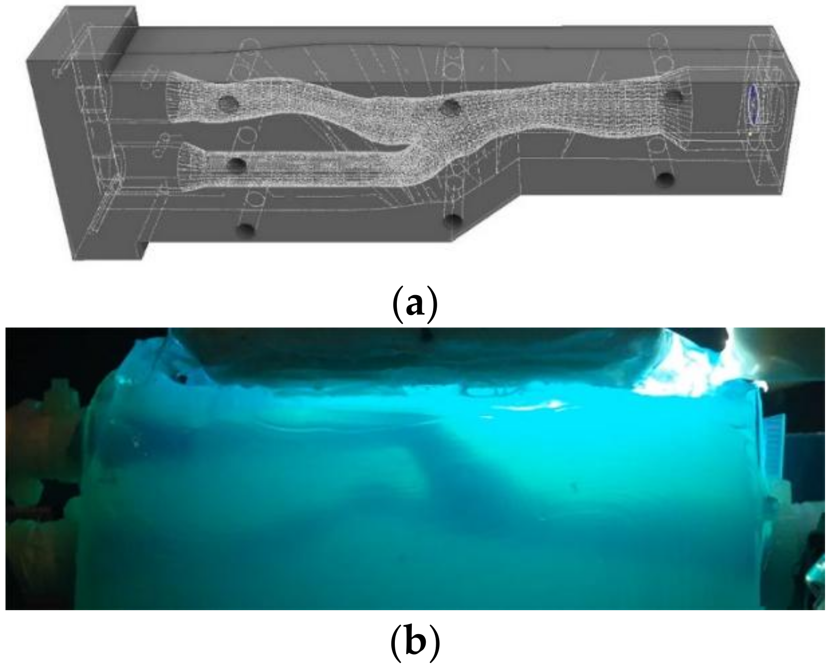
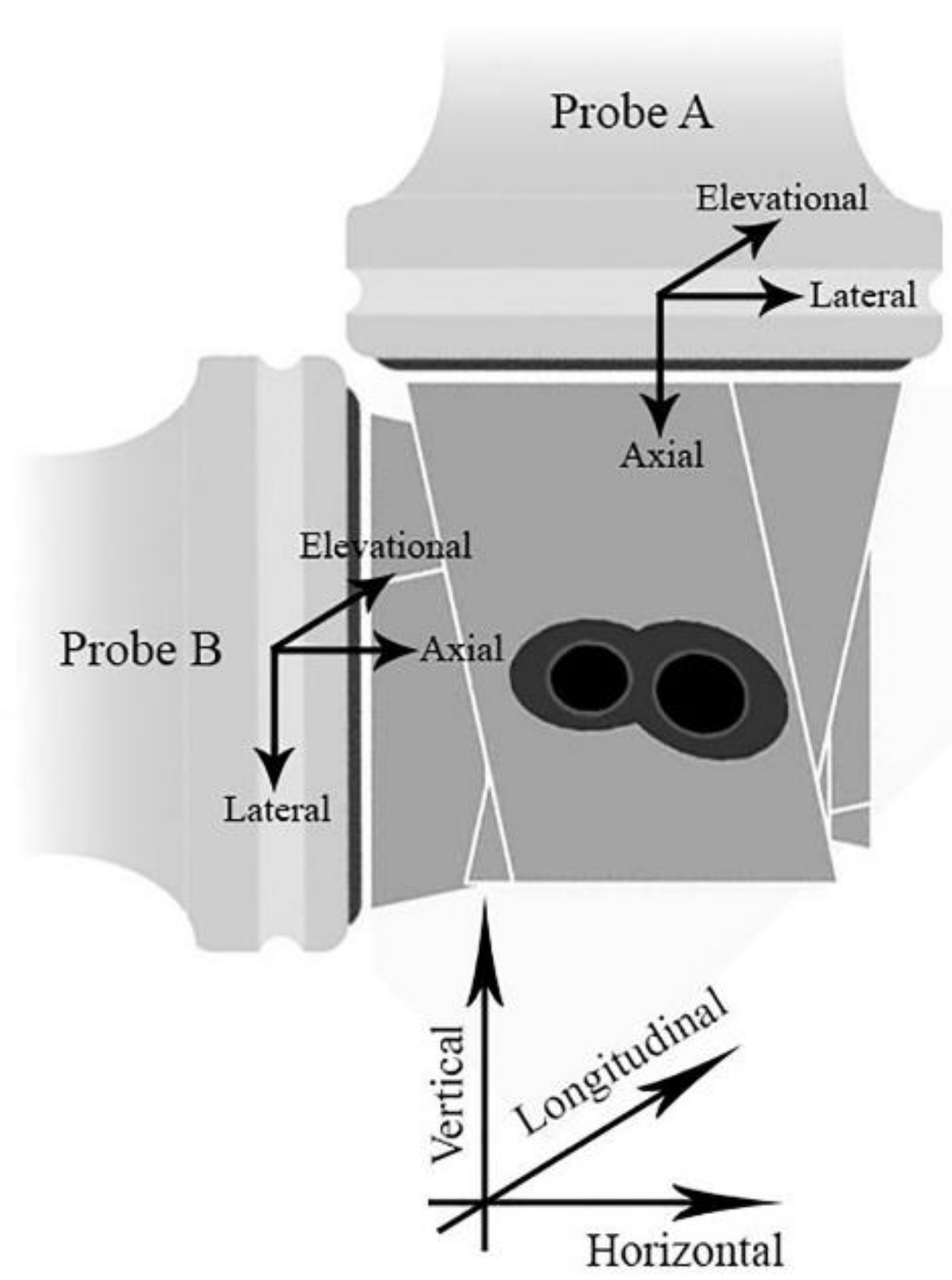
2.1. Experimental Setup
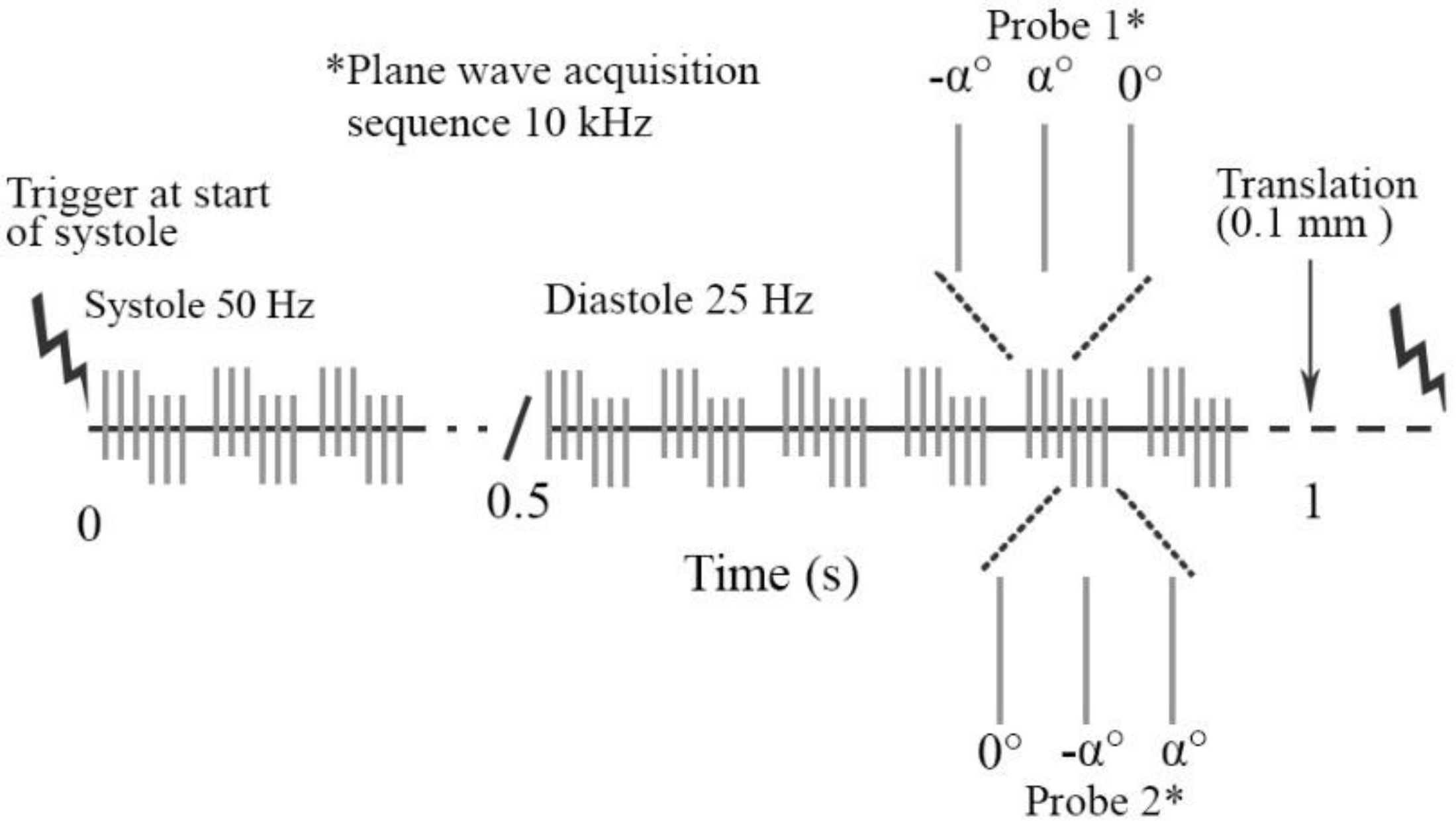
2.2. Ultrasound Data Acquisition
2.3. Post Processing RF Element Data
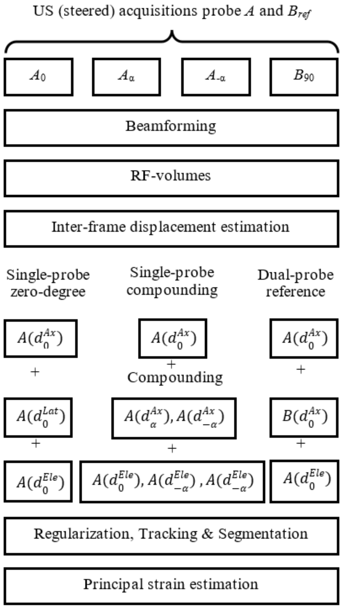
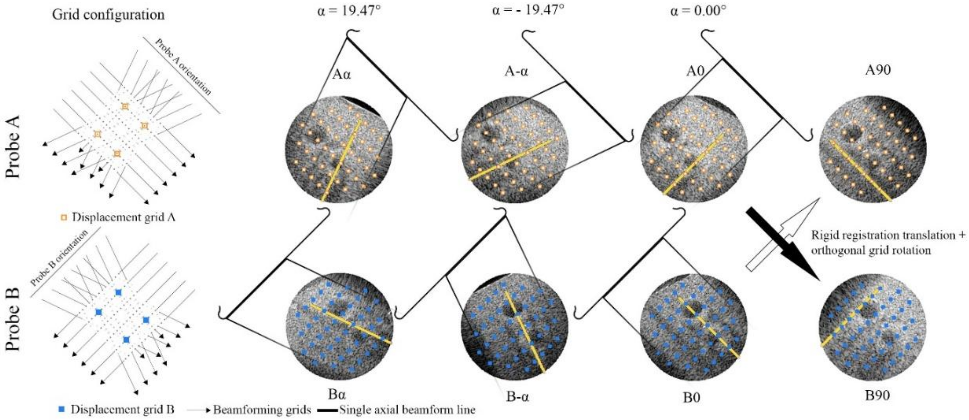
2.4. 3D Interframe Displacement Estimation
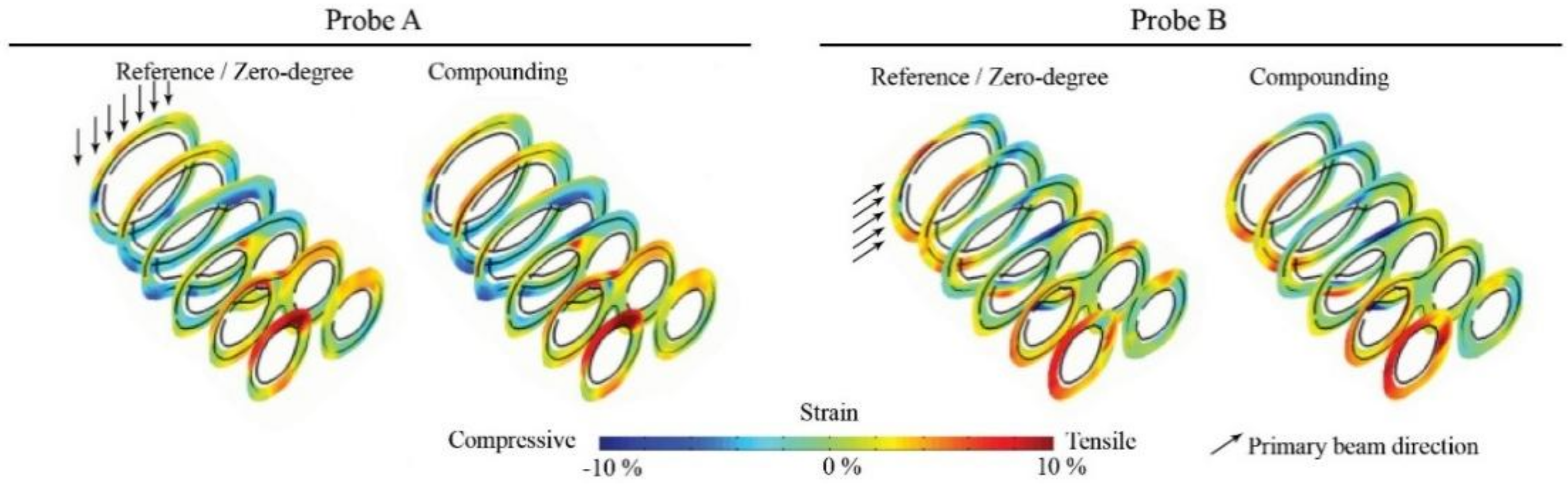
2.4.1. Single-Probe Zero-Degree
2.4.2. Single-Probe Compounding
2.4.3. Dual-Probe Reference
2.5. Regularization Tracking and Segmentation
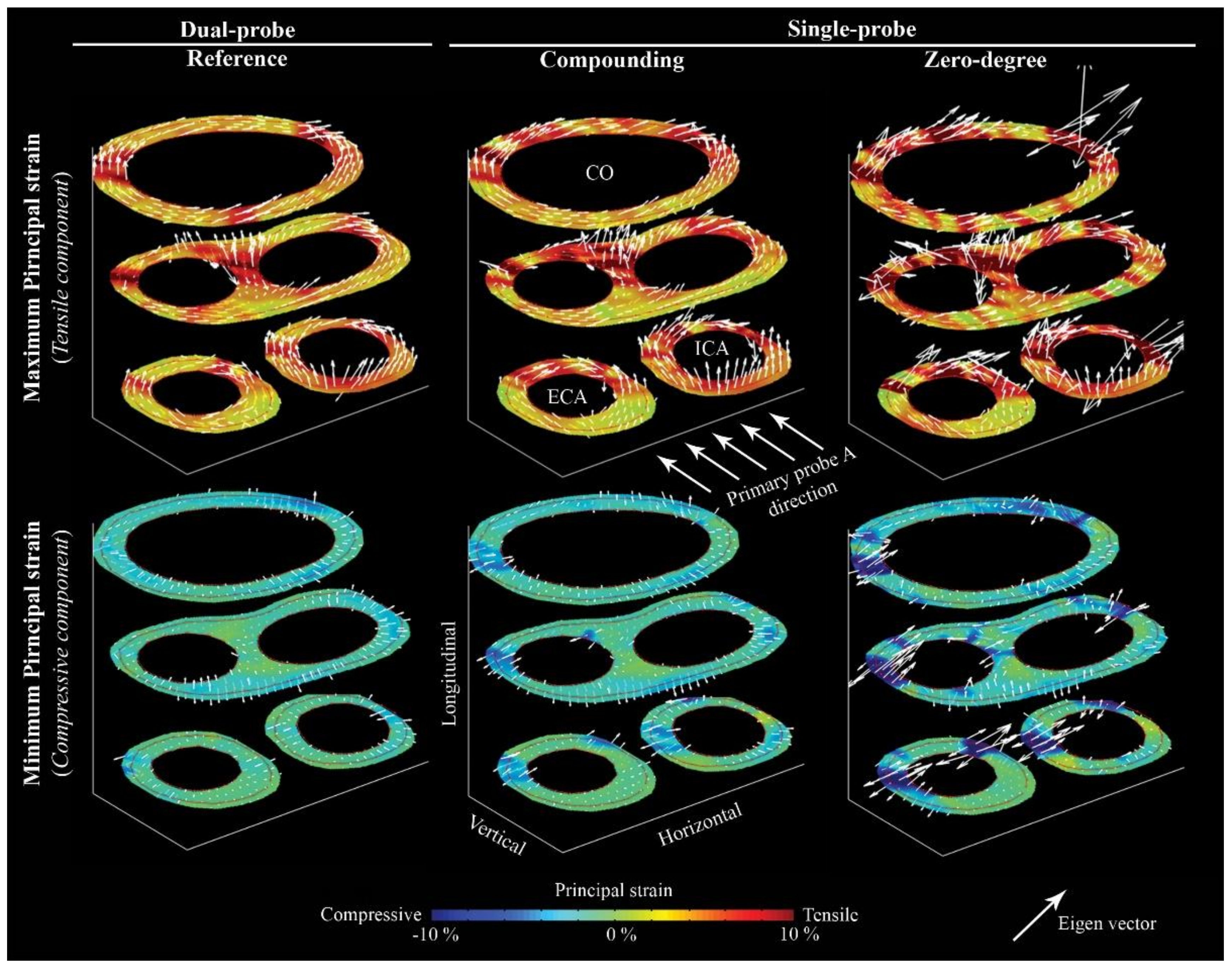
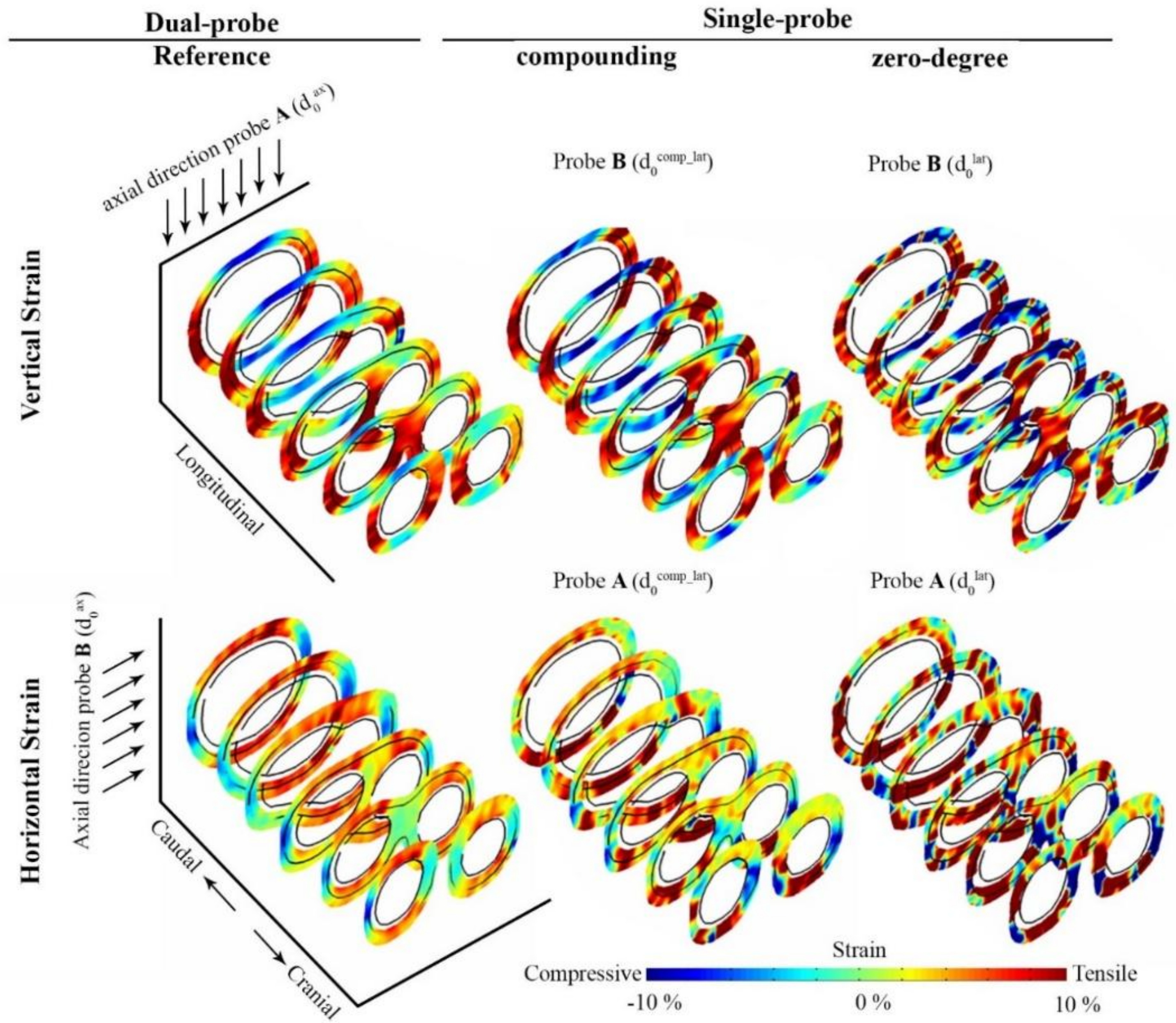
2.6. Strain Estimation
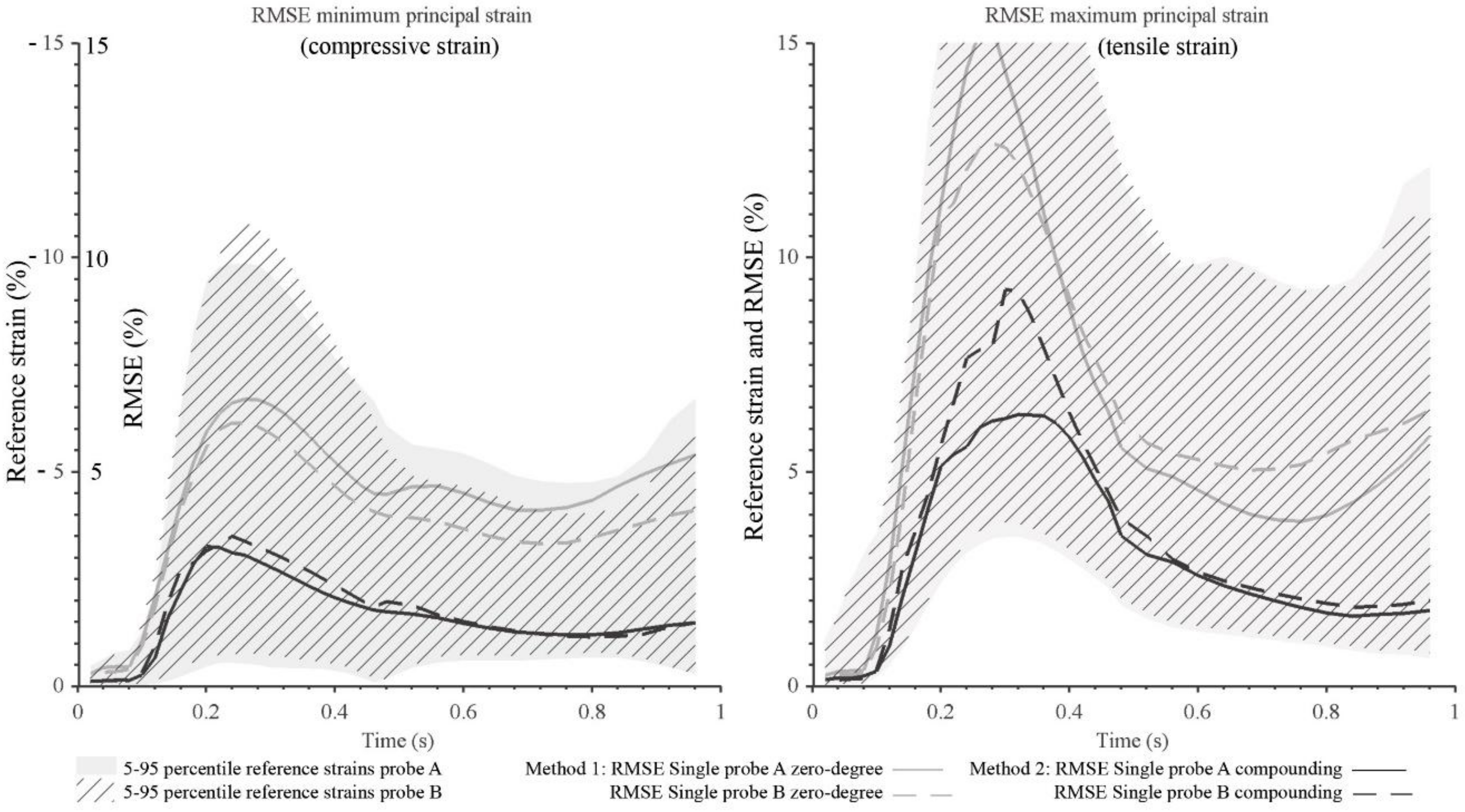
2.7. Evaluation
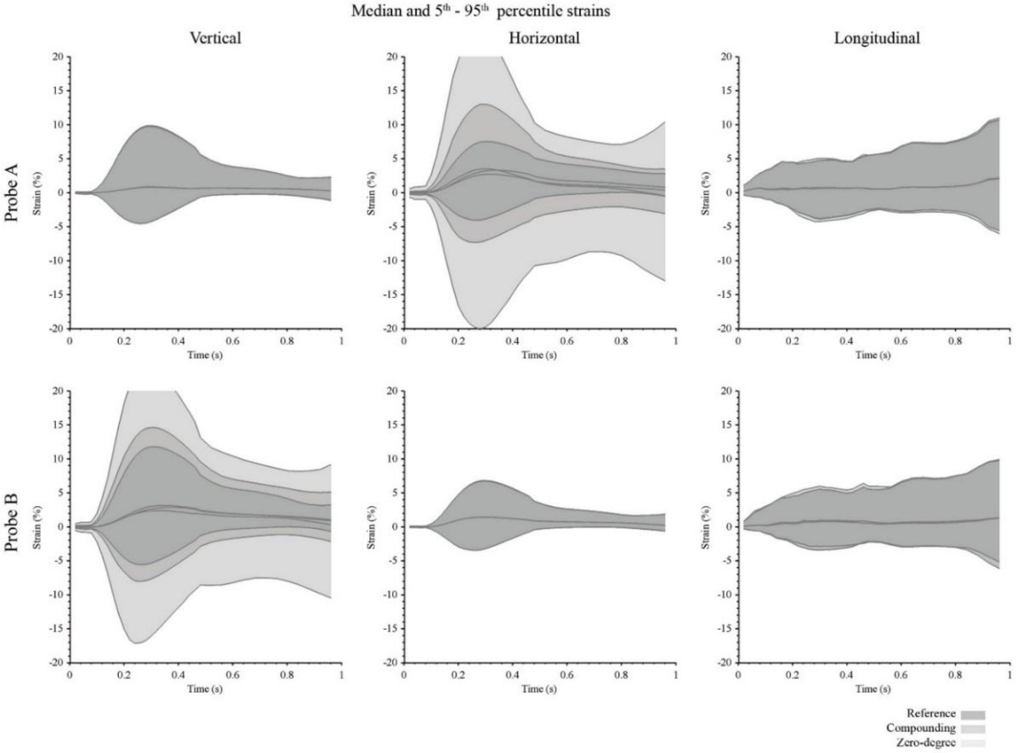
3. Results
4. Discussion
5. Conclusions
Supplementary Materials
Acknowledgments
Author Contributions
Conflicts of Interest
References
- Ophir, J.; Céspedes, I.; Ponnekanti, H.; Yazdi, Y.; Li, X. Elastography: A quantitative method for imaging the elasticity of biological tissues. Ultrason. Imaging 1991, 13, 111–134. [Google Scholar] [CrossRef] [PubMed]
- Hansen, H.H.; de Borst, G.J.; Bots, M.L.; Moll, F.L.; Pasterkamp, G.; de Korte, C.L. Validation of noninvasive in vivo compound ultrasound strain imaging using histologic plaque vulnerability features. Stroke 2016, 47, 2770–2775. [Google Scholar] [CrossRef] [PubMed]
- Ohayon, J.; Finet, G.; Le Floc’h, S.; Cloutier, G.; Gharib, A.M.; Heroux, J.; Pettigrew, R.I. Biomechanics of atherosclerotic coronary plaque: Site, stability and in vivo elasticity modeling. Ann. Biomed. Eng. 2014, 42, 269–279. [Google Scholar] [CrossRef] [PubMed] [Green Version]
- Cardinal, M.H.R.; Heusinkveld, M.H.G.; Qin, Z.; Lopata, R.G.P.; Naim, C.; Soulez, G.; Cloutier, G. Carotid artery plaque vulnerability assessment using noninvasive ultrasound elastography: Validation with MRI. Am. J. Roentgenol. 2017, 209, 142–151. [Google Scholar] [CrossRef] [PubMed]
- Huang, C.W.; He, Q.; Huang, M.W.; Huang, L.Y.; Zhao, X.H.; Yuan, C.; Luo, J.W. Non-invasive identification of vulnerable atherosclerotic plaques using texture analysis in ultrasound carotid elastography: An in vivo feasibility study validated by magnetic resonance imaging. Ultrasound Med. Biol. 2017, 43, 817–830. [Google Scholar] [CrossRef] [PubMed]
- Schaar, J.A.; Muller, J.E.; Falk, E.; Virmani, R.; Fuster, V.; Serruys, P.W.; Colombo, A.; Stefanadis, C.; Ambrose, J.A.; Moreno, P.; et al. Terminology for high-risk and vulnerable coronary artery plaques. Eur. Heart J. 2004, 25, 1077–1082. [Google Scholar] [CrossRef] [PubMed]
- Lendon, C.L.; Davies, M.J.; Born, G.V.R.; Richardson, P.D. Atherosclerotic plaque caps are locally weakened when macrophage density is increased. Atherosclerosis 1991, 87, 87–90. [Google Scholar] [CrossRef]
- Hellings, W.E.; Peeters, W.; Moll, F.L.; Piers, S.R.D.; van Setten, J.; Van der Spek, P.J.; de Vries, J.P.P.M.; Seldenrijk, K.A.; De Bruin, P.C.; Vink, A.; et al. Composition of carotid atherosclerotic plaque is associated with cardiovascular outcome a prognostic study. Circulation 2010, 121, 1941–1950. [Google Scholar] [CrossRef] [PubMed]
- De Korte, C.L.; Céspedes, E.I.; van der Steen, A.F.W.; Pasterkamp, G.; Bom, N. Intravascular ultrasound elastography: Assessment and imaging of elastic properties of diseased arteries and vulnerable plaque. Eur. J. Ultrasound 1998, 7, 219–224. [Google Scholar] [CrossRef]
- Ribbers, H.; Lopata, R.G.; Holewijn, S.; Pasterkamp, G.; Blankensteijn, J.D.; de Korte, C.L. Noninvasive two-dimensional strain imaging of arteries: Validation in phantoms and preliminary experience in carotid arteries in vivo. Ultrasound Med. Biol. 2007, 33, 530–540. [Google Scholar] [CrossRef] [PubMed]
- McCormick, M.; Varghese, T.; Wang, X.; Mitchell, C.; Kliewer, M.A.; Dempsey, R.J. Methods for robust in vivo strain estimation in the carotid artery. Phys. Med. Biol. 2012, 57, 7329–7353. [Google Scholar] [CrossRef] [PubMed]
- Schmitt, C.; Soulez, G.; Maurice, R.L.; Giroux, M.F.; Cloutier, G. Noninvasive vascular elastography: Toward a complementary characterization tool of atherosclerosis in carotid arteries. Ultrasound Med. Biol. 2007, 33, 1841–1858. [Google Scholar] [CrossRef] [PubMed]
- Kawasaki, T.; Fukuda, S.; Shimada, K.; Maeda, K.; Yoshida, K.; Sunada, H.; Inanami, H.; Tanaka, H.; Jissho, S.; Taguchi, H.; et al. Direct measurement of wall stiffness for carotid arteries by ultrasound strain imaging. J. Am. Soc. Echocardiogr. 2009, 22, 1389–1395. [Google Scholar] [CrossRef] [PubMed]
- Poree, J.; Chayer, B.; Soulez, G.; Ohayon, J.; Cloutier, G. Noninvasive vascular modulography method for imaging the local elasticity of atherosclerotic plaques: Simulation and in vitro vessel phantom study. IEEE Trans. Ultrason. Ferroelectr. Freq. Control 2017, 64, 1805–1817. [Google Scholar] [CrossRef] [PubMed]
- Khamdaeng, T.; Luo, J.; Vappou, J.; Terdtoon, P.; Konofagou, E.E. Arterial stiffness identification of the human carotid artery using the stress-strain relationship in vivo. Ultrasonics 2012, 52, 402–411. [Google Scholar] [CrossRef] [PubMed]
- De Korte, C.L.; Sierevogel, M.; Mastik, F.; Strijder, C.; Velema, E.; Pasterkamp, G.; van der Steen, A.F.W. Identification of atherosclerotic plaque components with intravascular ultrasound elastography in vivo: A yucatan pig study. Circulation 2002, 105, 1627–1630. [Google Scholar] [CrossRef] [PubMed]
- Kanai, H.; Hasegawa, H.; Ichiki, M.; Tezuka, F.; Koiwa, Y. Elasticity imaging of atheroma with transcutaneous ultrasound preliminary study. Circulation 2003, 107, 3018–3021. [Google Scholar] [CrossRef] [PubMed]
- Hansen, H.H.; Lopata, R.G.; Idzenga, T.; de Korte, C.L. Full 2d displacement vector and strain tensor estimation for superficial tissue using beam-steered ultrasound imaging. Phys. Med. Biol. 2010, 55, 3201–3218. [Google Scholar] [CrossRef] [PubMed]
- Hansen, H.H.; Saris, A.E.; Vaka, N.R.; Nillesen, M.M.; de Korte, C.L. Ultrafast vascular strain compounding using plane wave transmission. J. Biomech. 2014, 47, 815–823. [Google Scholar] [CrossRef] [PubMed] [Green Version]
- Korukonda, S.; Nayak, R.; Carson, N.; Schifitto, G.; Dogra, V.; Doyley, M.M. Noninvasive vascular elastography using plane-wave and sparse-array imaging. IEEE Trans. Ultrason. Ferroelectr. Freq. Control 2013, 60, 332–342. [Google Scholar] [CrossRef] [PubMed]
- Poree, J.; Garcia, D.; Chayer, B.; Ohayon, J.; Cloutier, G. Noninvasive vascular elastography with plane strain incompressibility assumption using ultrafast coherent compound plane wave imaging. IEEE Trans. Med. Imaging 2015, 34, 2618–2631. [Google Scholar] [CrossRef] [PubMed]
- Larsson, M.; Verbrugghe, P.; Smoljkic, M.; Verhoeven, J.; Heyde, B.; Famaey, N.; Herijgers, P.; D’Hooge, J. Strain assessment in the carotid artery wall using ultrasound speckle tracking: Validation in a sheep model. Phys. Med. Biol. 2015, 60, 1107–1123. [Google Scholar] [CrossRef] [PubMed]
- Fekkes, S.; Swillens, A.E.S.; Hansen, H.H.G.; Saris, A.E.C.M.; Nillesen, M.M.; Iannaccone, F.; Segers, P.; de Korte, C.L. 2-d versus 3-d cross-correlation-based radial and circumferential strain estimation using multiplane 2-d ultrafast ultrasound in a 3-d atherosclerotic carotid artery model. IEEE Trans. Ultrason. Ferroelectr. Freq. Control 2016, 63, 1543–1553. [Google Scholar] [CrossRef] [PubMed]
- Cinthio, M.; Ahlgren, A.R.; Bergkvist, J.; Jansson, T.; Persson, H.W.; Lindstrom, K. Longitudinal movements and resulting shear strain of the arterial wall. Am. J. Physiol. Heart Circ. Physiol. 2006, 291, H394–H402. [Google Scholar] [CrossRef] [PubMed]
- Svedlund, S.; Eklund, C.; Robertsson, P.; Lomsky, M.; Gan, L.M. Carotid artery longitudinal displacement predicts 1-year cardiovascular outcome in patients with suspected coronary artery disease. Arterioscler. Thromb. Vasc. Biol. 2011, 31, 1668–1674. [Google Scholar] [CrossRef] [PubMed]
- Landry, A.; Spence, J.D.; Fenster, A. Quantification of carotid plaque volume measurements using 3d ultrasound imaging. Ultrasound Med. Biol. 2005, 31, 751–762. [Google Scholar] [CrossRef] [PubMed]
- Steinke, W.; Hennerici, M. Three-dimensional ultrasound imaging of carotid artery plaques. J. Cardiovasc. Technol. 1989, 8, 15–22. [Google Scholar]
- Fenster, A.; Parraga, G.; Bax, J. Three-dimensional ultrasound scanning. Interface Focus 2011, 1, 503–519. [Google Scholar] [CrossRef] [PubMed]
- Baldassarre, D.; Amato, M.; Bondioli, A.; Sirtori, C.R.; Tremoli, E. Carotid artery intima-media thickness measured by ultrasonography in normal clinical practice correlates well with atherosclerosis risk factors. Stroke 2000, 31, 2426–2430. [Google Scholar] [CrossRef] [PubMed]
- Landry, A.; Spence, J.D.; Fenster, A. Measurement of carotid plaque volume by 3-dimensional ultrasound. Stroke 2004, 35, 864–869. [Google Scholar] [CrossRef] [PubMed]
- Delcker, A.; Diener, H.C. 3d ultrasound measurement of atherosclerotic plaque volume in carotid arteries. Bildgeb. Imaging 1994, 61, 116–121. [Google Scholar]
- Boekhoven, R.W.; Rutten, M.C.M.; van Sambeek, M.R.; van de Vosse, F.N.; Lopata, R.G.P. Towards mechanical characterization of intact endarterectomy samples of carotid arteries during inflation using echo-ct. J. Biomech. 2014, 47, 805–814. [Google Scholar] [CrossRef] [PubMed]
- Boekhoven, R.W.; Rutten, M.C.M.; van Sambeek, M.R.; van de Vosse, F.N.; Lopata, R.G.P. Echo-computed tomography strain imaging of healthy and diseased carotid specimens. Ultrasound Med. Biol. 2014, 40, 1329–1342. [Google Scholar] [CrossRef] [PubMed]
- Liang, Y.; Zhu, H.; Friedman, M.H. Measurement of the 3d arterial wall strain tensor using intravascular b-mode ultrasound images: A feasibility study. Phys. Med. Biol. 2010, 55, 6377–6394. [Google Scholar] [CrossRef] [PubMed]
- Hansen, H.H.; de Borst, G.J.; Bots, M.L.; Moll, F.L.; Pasterkamp, G.; de Korte, C.L. Compound ultrasound strain imaging for noninvasive detection of (fibro)atheromatous plaques: Histopathological validation in human carotid arteries. JACC Cardiovasc. Imaging 2016, 9, 1466–1467. [Google Scholar] [CrossRef] [PubMed]
- Nayak, R.; Huntzicker, S.; Ohayon, J.; Carson, N.; Dogra, V.; Schifitto, G.; Doyley, M.M. Principal strain vascular elastography: Simulation and preliminary clinical evaluation. Ultrasound Med. Biol. 2017, 43, 682–699. [Google Scholar] [CrossRef] [PubMed]
- Fromageau, J.; Gennisson, J.L.; Schmitt, C.; Maurice, R.L.; Mongrain, R.; Cloutier, G. Estimation of polyvinyl alcohol cryogel mechanical properties with four ultrasound elastography methods and comparison with gold standard testings. IEEE Trans. Ultrason. Ferroelectr. Freq. Control 2007, 54, 498–509. [Google Scholar] [CrossRef] [PubMed]
- Hansen, H.H.G.; Lopata, R.G.P.; Idzenga, T.; De Korte, C.L. Fast strain tensor imaging using beam steered plane wave ultrasound transmissions. In Proceedings of the 2010 IEEE International Ultrasonics Symposium (IUS), San Diego, CA, USA, 11–14 October 2010; pp. 1344–1347. [Google Scholar]
- Akyildiz, A.C.; Speelman, L.; Gijsen, F.J.H. Mechanical properties of human atherosclerotic intima tissue. J. Biomech. 2014, 47, 773–783. [Google Scholar] [CrossRef] [PubMed]
- Varghese, T.; Ophir, J. A theoretical framework for performance characterization of elastography: The strain filter. IEEE Trans. Ultrason. Ferroelectr. Freq. Control 1997, 44, 164–172. [Google Scholar] [CrossRef] [PubMed]
- Saris, A.E.C.M.; Nillesen, M.M.; Fekkes, S.; Hansen, H.H.G.; de Korte, C.L. Robust blood velocity estimation using point-spread-function-based beamforming and multi-step speckle tracking. In Proceedings of the 2015 IEEE International Ultrasonics Symposium (IUS), Taipei, Taiwan, 21–24 October 2015; pp. 1–4. [Google Scholar]
- Kim, S.; Aglyamov, S.R.; Park, S.; O’Donnell, M.; Emelianov, S.Y. An autocorrelation-based method for improvement of sub-pixel displacement estimation in ultrasound strain imaging. IEEE Trans. Ultrason. Ferroelectr. Freq. Control 2011, 58, 838–843. [Google Scholar] [PubMed]
- Kallel, F.; Ophir, J. A least-squares strain estimator for elastography. Ultrason. Imaging 1997, 19, 195–208. [Google Scholar] [CrossRef] [PubMed]
- Chee, A.J.Y.; Ho, C.K.; Yiu, B.Y.S.; Yu, A.C.H. Walled carotid bifurcation phantoms for imaging investigations of vessel wall motion and blood flow dynamics. IEEE Trans. Ultrason. Ferroelectr. Freq. Control 2016, 63, 1852–1864. [Google Scholar] [CrossRef] [PubMed]
- Boekhoven, R.W.; Rutten, M.C.M.; van de Vosse, F.N.; Lopata, R.G.P. Design of a fatty plaque phantom for validation of strain imaging. In Proceedings of the 2014 IEEE International Ultrasonics Symposium, Chicago, IL, USA, 3–6 September 2014; pp. 2619–2622. [Google Scholar]
- Liu, Y.; Dang, C.; Garcia, M.; Gregersen, H.; Kassab, G.S. Surrounding tissues affect the passive mechanics of the vessel wall: Theory and experiment. Am. J. Physiol. Heart C 2007, 293, H3290–H3300. [Google Scholar] [CrossRef] [PubMed]
- Berne, R.M.; Levy, M.N. Physiology, 3rd ed.; Mosby Year Book: Saint Louis, France, 1993. [Google Scholar]


| Beamforming Grid (µm) | Displacement Grid (µm) | ||
|---|---|---|---|
| Zero-Degree | −α, +α, Orthogonal | ||
| dx | 64.2 | 30.2 | 64.2 |
| dy | 10.1 | 10.7 | 9.1 |
| dz | 100 | 100 | 100 |
| Axis Direction | 3D Interframe Displacement Estimation | 3D Strain Estimation | |||||
|---|---|---|---|---|---|---|---|
| Window Size ± Search Range (Beamforming Grid Samples) | Regularization (Displacement Grid Samples) | Least Square Window Sizes (Ax, Lat, Ele) | |||||
| Sample Iteration | Sub-Sample Iteration | Median Filtering (Kernel Sample Size Ax, Lat, Ele) | |||||
| Inter–Frame | Tracked | Ax | Lat | Ele | |||
| Axial | 81 ± 15 | 33 ± 5 | 7, 11, 3 | 7, 11, 3 | 17, 7, 3 | 5, 25,3 | 5, 7, 15 |
| Lateral | 13 ± 4 | 7 ± 4 | 7, 11, 3 | 7, 11, 3 | 17, 7, 3 | 5, 25, 3 | 5, 7, 15 |
| Elevational | 3 ± 0 | 3 ± 2 | 28, 20, 5 | 7, 11, 3 | 33, 11, 7 | 9, 49, 7 | 9, 11, 61 |
| Strain (%) at Max. Systolic Pressure t = 0.30 s | Residual Strain (%) t = 0.96 s | ||||||
|---|---|---|---|---|---|---|---|
| Probe | Reference | Compounding | Zero-Degree | Reference | Compounding | Zero-Degree | |
| Vertical | A | −4.2–9.7 | −4.3–9.8 | −4.9–9.7 | −1.1–2.3 | −1.1–2.3 | −1.2–2.3 |
| B | −5.3–11.8 | −7.6–14.6 | −16.0–23.0 | −0.7–3.2 | −2.2–5.1 | −10.5–9.1 | |
| Horizontal | A | −3.9–7.5 | −7.0–13.0 | −19.7–23.6 | −0.5–2.8 | −3.1–3.5 | −13.1–0.4 |
| B | −3.2–6.8 | −3.2–6.7 | −3.2–6.7 | −0.6–1.8 | −0.6–1.9 | −0.6–1.8 | |
| Longitudinal | A | −3.8–4.7 | −4.3–5.0 | −3.9–4.7 | −5.6–10.7 | −6.0–11.0 | −5.6–10.7 |
| B | −3.4–5.5 | −2.9–6.0 | −3.4–5.5 | −6.1–9.9 | −5.2–9.8 | −6.1–9.9 | |
© 2018 by the authors. Licensee MDPI, Basel, Switzerland. This article is an open access article distributed under the terms and conditions of the Creative Commons Attribution (CC BY) license (http://creativecommons.org/licenses/by/4.0/).
Share and Cite
Fekkes, S.; Saris, A.E.C.M.; Menssen, J.; Nillesen, M.M.; Hansen, H.H.G.; De Korte, C.L. Multi-Plane Ultrafast Compound 3D Strain Imaging: Experimental Validation in a Carotid Bifurcation Phantom. Appl. Sci. 2018, 8, 637. https://doi.org/10.3390/app8040637
Fekkes S, Saris AECM, Menssen J, Nillesen MM, Hansen HHG, De Korte CL. Multi-Plane Ultrafast Compound 3D Strain Imaging: Experimental Validation in a Carotid Bifurcation Phantom. Applied Sciences. 2018; 8(4):637. https://doi.org/10.3390/app8040637
Chicago/Turabian StyleFekkes, Stein, Anne E. C. M. Saris, Jan Menssen, Maartje M. Nillesen, Hendrik H. G. Hansen, and Chris L. De Korte. 2018. "Multi-Plane Ultrafast Compound 3D Strain Imaging: Experimental Validation in a Carotid Bifurcation Phantom" Applied Sciences 8, no. 4: 637. https://doi.org/10.3390/app8040637