A Nonlinear Beamformer Based on p-th Root Compression—Application to Plane Wave Ultrasound Imaging
by
 ,
,
Maxime Polichetti
1,2,*, 
François Varray
1,
Jean-Christophe Béra
2,
Christian Cachard
1 and
Barbara Nicolas
1 1
University Lyon, INSA-Lyon, UCBL, UJM-Saint-Etienne, CNRS, Inserm, CREATIS UMR 5220, U1206, F-69100 Villeurbanne, France
2
LabTAU, INSERM, Centre Léon Bérard, UCBL, University Lyon, F-69003 Lyon, France
*
Author to whom correspondence should be addressed.
Appl. Sci. 2018, 8(4), 599; https://doi.org/10.3390/app8040599
Submission received: 23 February 2018
/
Revised: 27 March 2018
/
Accepted: 31 March 2018
/
Published: 11 April 2018
(This article belongs to the Special Issue Ultrasound B-mode Imaging: Beamforming and Image Formation Techniques)
Abstract
:Ultrafast medical ultrasound imaging is necessary for 3D and 4D ultrasound imaging, and it can also achieve high temporal resolution (thousands of frames per second) for monitoring of transient biological phenomena. However, reaching such frame rates involves reduction of image quality compared with that obtained with conventional ultrasound imaging, since the latter requires each image line to be reconstructed separately with a thin ultrasonic focused beam. There are many techniques to simultaneously acquire several image lines, although at the expense of resolution and contrast, due to interference from echoes from the whole medium. In this paper, a nonlinear beamformer is applied to plane wave imaging to improve resolution and contrast of ultrasound images. The method consists of the introduction of nonlinear operations in the conventional delay-and-sum (DAS) beamforming algorithm. To recover the value of each pixel, the raw radiofrequency signals are first dynamically focused and summed on the plane wave dimension. Then, their amplitudes are compressed using the signed root. After summing on the element dimension, the signed p-power is applied to restore the original dimensionality in volts. Finally, a band-pass filter is used to remove artificial harmonics introduced by these nonlinear operations. The proposed method is referred to as p-DAS, and it has been tested here on numerical and experimental data from the open access platform of the Plane wave Imaging Challenge in Medical UltraSound (PICMUS). This study demonstrates that p-DAS achieves better resolution and artifact rejection than the conventional DAS (for with eleven plane wave imaging on experimental phantoms, the lateral resolution is improved by , and contrast ratio (CR) by ). However, like many coherence-based beamformers, it tends to distort the conventional speckle structure (contrast-to-noise-ratio (CNR) decreased by ). It is demonstrated that p-DAS, for , is very similar to the nonlinear filtered-delay-multiply-and-sum (FDMAS) beamforming, but also that its impact on image quality can be tuned changing the value of p.
1. Introduction
In ultrasound B-mode imaging, in terms of resolution and contrast, the image quality relies essentially on the strategy used to sonicate the biological tissue. The conventional focused approach consists of constructing the image lines one by one. Such approach suffers from particularly low frame rates (tens of frames per second) that are then not compatible with the present issues of ultrafast medical imaging allowing thousands of frames per second necessary for the the observation of transient biological phenomena [1], but also three-dimensional (3D), and even 4D, imaging [2].
To increase the frame rate, different sonication strategies have been investigated to decrease the number of acquisitions required to obtain a complete image. Multi-line acquisition uses wider beams for reconstruction, with several adjacent lines at the same time [3]. The multi-line transmit strategy consists of transmitting L simultaneous focused beams to reconstruct L image lines at the same time [4]. In both cases, the frame rate is multiplied by the number of simultaneous reconstructed lines. However, the image quality is impacted upon, due to interference from the echoes of different image lines.
To go further, all of the image lines can be reconstructed using the same set of radiofrequency (RF) signals after the whole medium has been sonicated with a single plane wave. In this case, the frame rate is multiplied by the number of image lines, which allows the acquisition of thousands of images per second. However, as less energy is sent into the medium and the echoes from the medium interfere, the resolution and the contrast are degraded. To limit this impact on image quality, several transmissions/receptions of steered plane waves can be combined to reconstruct a single image [5]. Montaldo et al. demonstrated that the image quality obtained with the conventional focused beam strategy can be recovered with plane wave compounding using a 10-fold greater frame rate. However, in the context of ultrafast imaging, the number of plane waves must be maintained as low as possible, and so image quality needs to be achieved with a complementary approach.
In addition, image quality relies on the beamformer used for reception, in order to process the raw echo signals into image lines. The conventional delay-and-sum (DAS) beamformer consists of correctly rephasing the raw signals acquired with the probe, and simply summing these. However, better resolution and contrast can be achieved by combining the delayed signals in a different way. The basic approach consists of applying a fixed weighting window before the sum of the delayed signals, to influence the shape of the point spread function (PSF). Typically, Tukey, Hann, or Hamming windows are used to reduce the side-lobe level, at the expense of a wider main lobe. Tong et al. investigated the influence of window shape on the rejection of interference during reception [4]. To go further, the adaptive Capon’s minimum variance beamformer was proposed to compute the optimal weighting window that corresponds to each pixel [6,7]. This approach achieves a lot thinner main lobe and strong side-lobe rejection, compared with conventional DAS. Nevertheless, since finding the optimal set of weights for each pixel involves high computational complexity, the computing time required for beamforming is no more negligible than for simple DAS. A derived approach with lower complexity level was proposed by [8]. The optimal window for each pixel is chosen from a predefined set of windows. As the number of predefined windows increases, the image quality is enhanced, while the computational costs rise.
Other adaptive beamformers are instead based on coherence. These can reduce artifacts that originate from incoherent noise or interference. The coherence of N delayed samples is measured to obtain a weighting factor that is associated to each pixel value computed with the DAS beamformer. For instance, the generalized coherence factor is computed on the fast Fourier transform of the aperture [9], in order to define the coherent energy in the low frequencies. Alternatively, the phase coherence factor tends to reject the pixel value when the phase dispersion is high through the aperture [10]. The resolution and contrast enhancement, coupled with the low level of complexity (suitable for real-time implementation), make coherence approaches very attractive.
Recently, Matrone et al. proposed a nonlinear beamformer to enhance image quality, known as filtered-delay multiply-and-sum (FDMAS) [11], and demonstrated that this can be used to reject interference in the case of multi-line transmit imaging [12]. As this process correlates the N delayed samples, FDMAS can be considered as a beamformer that is based on coherence [13]. The value of each pixel is computed as the sum of the signed square roots of the corresponding N delayed samples, multiplied in pairs. The signed square root is used to keep the original pixel dimensionality in volts. However, these cross-products represent heavy computational costs.
A previous study demonstrated that the algebraic expression of FDMAS can be approximated as the squared sum of the signed square roots of the delayed samples [14]. Such formalism allows not only very similar performances of FDMAS to be recovered particularly rapidly, but also generalizes this approach to higher ranges by using the root. However, for even p-values, the sign of the oscillations is lost, which leads to the splitting of the frequency between the direct current (DC) components, and a doubling of the excitation frequency. This phenomenon tends to flatten the main lobe of the PSF compared to conventional DAS.
In the present study, a nonlinear beamformer is proposed, p-DAS, which consists of computing the value of each pixel as the signed p-power of the sum of the signed root of the delayed samples. As the signs of the ultrasound oscillations are preserved through the algorithm, the frequency content is no longer split.
This paper is organized as follows. In the second section, the beamformers compared for this study are introduced in the context of ultrafast plane wave imaging, as DAS (conventional), FDMAS (nonlinear), and p-DAS (proposed method). Then, the numerical and experimental settings for the reconstruction of the Plane-Wave Imaging Challenge in Medical Ultrasound (PICMUS; IEEE IUS 2016) data [15] are described. In the third section, the principle and performance of p-DAS are illustrated. The last section concludes the paper and looks at several perspectives for the proposed method.
2. Methods and Materials
In this section, the three beamformers that are compared are presented in the context of plane wave compounding [5] (note that p-DAS beamforming could be applied to synthetic aperture or conventional focused imaging). Then, conventional DAS and FDMAS, as proposed by [11], and the here-proposed p-DAS method, are described. The data settings and reconstruction parameters are also given.
2.1. Methods
2.1.1. Conventional DAS for Plane Wave Imaging
In this section, the process for compounded plane wave imaging is described. The same linear ultrasound probe composed of N equally spaced elements is used for both transmission and reception. To reconstruct one image, M plane waves are transmitted. For a given plane wave m, with a transmission angle and a given element n of the array, the recorded signal is . The data acquired are beamformed to reconstruct the pixels in the grid , where x is the lateral axis parallel to the array, and z is the depth axis.
Each pixel of the RF image is obtained through combination of the correctly delayed samples . Each pixel is extracted from the raw echo signal . To correctly select the samples, two assumptions are required. The speed of sound in tissues is believed to be constant m·s, and a point scatterer is believed to back-scatter the spherical wave front. In this way, the echo back-scattered by a point located at corresponds to the samples with:
where is the time of flight of the wave, which is the sum of , the time in transmission for the steered plane wave m to get to the scatterer, and , the time in reception from the scatterer to element n of the probe:
where is the lateral position of the element. Then, the correctly delayed samples are summed on the plane wave dimension, in order to obtain N compounded delayed samples :
Finally, in the case of conventional DAS beamforming, the samples are simply summed along the element dimension, in order to obtain the pixel value :
where are the weighting coefficients of the apodization window (e.g., Tukey, Hann, and others). Finally, to obtain the B-mode image, the RF image is subjected to envelop detection along the depth dimension. Of note, if the central frequency of the ultrasound array is , then the RF image lines oscillate around the spatial frequency . Thus, for the sake of simplicity, the parts that follow make direct use of the temporal frequency rather than the spatial frequency .
In this study, all of the beamformers presented follow the same process for delaying and plane wave compounding. The only difference lies in the way are combined to obtain the pixel value .
2.1.2. FDMAS Beamforming
For FDMAS beamforming, as proposed by [11], each pixel is reconstructed by multiplying the compounded delayed samples in pairs. To keep the pixel dimensionality in volts, the signed square root is initially applied:
The value of the pixel computed by FDMAS reflects an autocorrelation process for the receive aperture. In this way, FDMAS rejects noise and incoherent echoes with greater efficiency than DAS. Note that the multiplication of signals with the same polarity leads to the loss of the sign information. Therefore, if the RF signals oscillate at (along the depth dimension), the spectrum of the image is split between the DC component and . To retrieve narrow-band image lines before envelop detection, the RF image needs to be band-pass filtered at along the depth dimension.
2.1.3. Proposed Method: p-DAS Beamforming
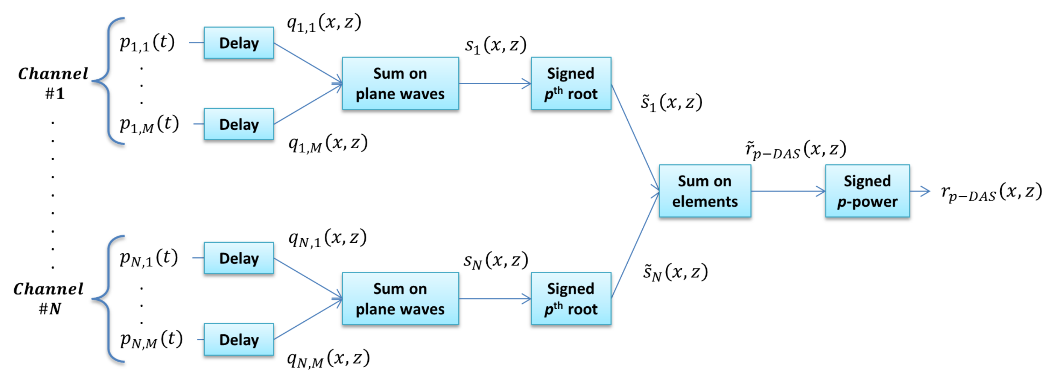
The proposed method is referred to as p-DAS. A block diagram is given in Figure 1 to describe how the value of a pixel is computed from the corresponding compounded delayed samples with the p-DAS beamformer. After being correctly delayed and compounded, the amplitudes are compressed through the application of the signed root:
Note that the p-value can be an integer or a float. Then, the are summed on the element dimension:
With the original dimensionality of in volts, this implies that is homogeneous to volt. Thus, p-powering is necessary to recover the conventional image dimensionality in volts, as for DAS. Note that the signed p-power is used to keep the polarity of the samples. The value of the pixel obtained is then:
Note that while oscillates at along the depth dimension, the nonlinear operations (such as signed root and signed p-power) distort the shape of oscillations, and so generate artificial harmonics on which have no acoustic meaning. The reconstructed image must be band-pass filtered to remove these artificial harmonics. The central frequency of this band-pass filter along the z-dimension is . Note also that the frequency sampling has to be high enough (e.g., ) to ignore the potential aliasing of artificial harmonics.
As for FDMAS, p-DAS is a coherence-based nonlinear beamformer, but it has the advantage that it is tunable with the p-value to balance the effects of the beamformer on the images. Moreover, p-DAS preserves the sign of the oscillations through the reconstruction process thanks to the use of the signed root and the signed p-power. Such difference and the impact on the images are investigated in Section 3.3.
In actuality, p-DAS can be viewed as DAS applied to the signed root of the raw signals, followed by the signed p-power, in order to re-establish the original dimension of the image. In this way, the effects of the coherent summation are reinforced. The principle of the proposed method is illustrated in Section 3.1, considering p-DAS as a DAS beamformer with adaptive weighting, as in [6]. Indeed, Equation (9) can be rearranged as:
where are the adaptive weights that depend on the amplitudes:
2.2. Materials
The performances of DAS, FDMAS, and p-DAS are compared based on the data acquired for the four phantoms available on the open access PICMUS platform (IEEE IUS 2016) [15]. The PICMUS challenge was specifically developed for a challenge on advanced beamforming methods using quantitative criteria for image quality. In this way, resolution and contrast are evaluated separately on two numerical phantoms and two experimental phantoms, using Matlab (R2016b, The MathWorks, Natick, MA, USA). The probe settings and the parameters for transmission are given in Table 1. The performances are evaluated with single plane wave imaging (1 PW), and also with 11 plane wave imaging (11 PW), uniformly tilted from to .
2.2.1. Beamforming Parameters
This part describes the details and parameters used for the three beamformers compared: DAS, FDMAS, and p-DAS. For all of these beamformers, the raw RF data are previously oversampled at MHz (corresponding to ). For this paper, the over sampling frequency was empirically determined to ignore the potential aliasing of artificial harmonics when using p-DAS. A dynamic aperture with a constant F-number of 1.75 is used, as by [5]. For DAS, uniform receive apodization is used. For FDMAS, the band-pass filter used is the same as that described by [16], as a Kaiser finite impulse response (FIR) filter with a centred frequency at and a pass-band defined on the range . For p-DAS, two p-values are investigated: and . The band-pass filter required to remove artificial harmonics on the image is performed along the depth dimension. The RF image is first low-pass filtered using a Butterworth filter (order 11; cut-off frequency ), and then it is high-pass filtered using another Butterworth filter (order 11; cut-off frequency ).
2.2.2. Image Quality Metrics
To evaluate image quality, the metrics are computed for the envelop images (before log-compression). The mean resolutions in the axial and lateral directions are automatically measured as described in [15]: the full width at half maximum (FWHM) is averaged over the 20 point scatterers for the numerical phantom (Figure 2a–d), and over seven point scatterers embedded in the speckle for experimental phantom (Figure 2i–l). This averaging is necessary as the FWHM is not spatially constant [17]. The contrast is measured according to two criteria: the mean contrast ratio (CR), and the mean contrast-to-noise ratio (CNR):
where k is the index of the cyst. (respectively ) is the mean pixel amplitude in the speckle ring (respectively inside the cyst). (respectively ) is the variance of the pixel amplitude in the speckle ring (respectively inside the cyst). For simulation, the phantom is composed of K = 9 cysts (Figure 2e–h), and, for the experiment, the phantom is composed of K = 2 cysts (Figure 2m–p). The full details of this dataset are available in [15].
3. Results and Discussion
In this section, the three beamformers (i.e., DAS, FDMAS, p-DAS) are analyzed and compared through the results obtained in simulation and experiments. In the first subsection, p-DAS is illustrated with a simulated point target. Then, the performances of the p-DAS in terms of the image quality (resolution and contrast) for the four phantoms of the PICMUS challenge are presented, for 1 PW and 11 PW. The last subsection makes the comparison of images reconstructed with FDMAS and p-DAS beamformers.
3.1. Analysis on the Principle of p-DAS
First of all, the principle of the p-DAS beamformer is compared to the DAS beamformer, for the case of single plane wave imaging. Namely, their respective PSFs (shown in Figure 3a,b) are investigated in simulation on the resolution phantom described by [15]. Here, p-DAS is considered as a DAS beamformer with adaptive weighting, considering Equations (11) and (12).
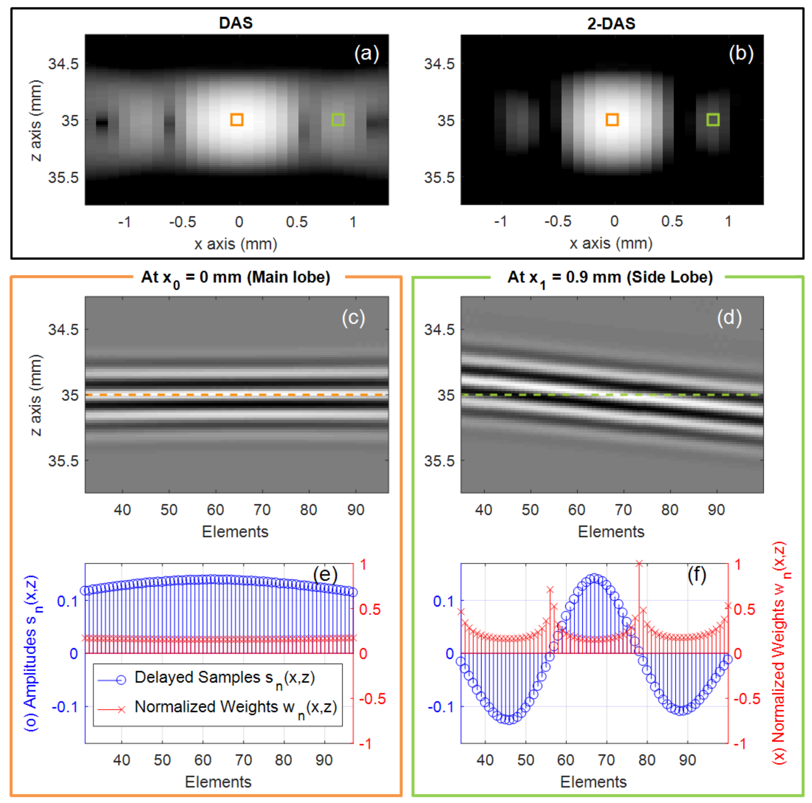
For the point scatterer placed at ( mm, mm), the PSF obtained with 2-DAS is shown in Figure 3b, and this shows better side-lobe rejection compared with the PSF obtained with DAS, as shown in Figure 3a. To explain this observation, the two beamformers are compared through consideration of two specific pixels: the maximum of the main lobe at ( mm, mm), which corresponds to the point scatterer location, and the peak side-lobe at ( mm, mm). First, the pixel reconstruction at the main lobe is investigated. In Figure 3c, the oscillations are successfully rephased for the pixel at () because a wave front actually comes from this location. As a result, a uniform level of amplitude is observed for in Figure 3e (blue). For DAS, these delayed samples are simply summed. For 2-DAS, an adaptive weighting window is applied (Figure 3e, red). However, the N weighting values are quasi-identical, as they depend on the amplitudes, which are similar along the elements. Finally, this pixel reconstructed with 2-DAS is equivalent to that reconstructed with DAS.
Then, DAS and 2-DAS are compared for the pixel at ( mm, mm), which corresponds to the peak side-lobe position for the reconstruction with DAS. The value of the pixel should tend to 0, as no scatterer is present. However, it is corrupted with the energy of the ill-rephased wave front in Figure 3d. As a result, the corresponding amplitudes are no longer uniform (Figure 3f, blue). To lower the value of the pixel reached with conventional DAS, the adaptive weights of 2-DAS tend to be the strongest for the lowest amplitudes, as demonstrated in Equation (12). This is why side-lobes vanish for 2-DAS (Figure 3b) compared to DAS (Figure 3a).
Note that, considering Equation (12), the side-lobe rejection increases with the p-value, as stronger weights are applied. The following subsection presents the impact on the B-mode images that arises from this adaptive approach.
3.2. Performances Evaluation of p-DAS on Image Quality
In this subsection, the image qualities obtained with the DAS and p-DAS ( and ) beamformers are investigated, in order to understand the influence of the value of p on images. The images obtained for single plane wave imaging (1 PW), and 11 plane wave imaging (11 PW) are presented and analyzed.
3.2.1. Single Plane Wave Imaging
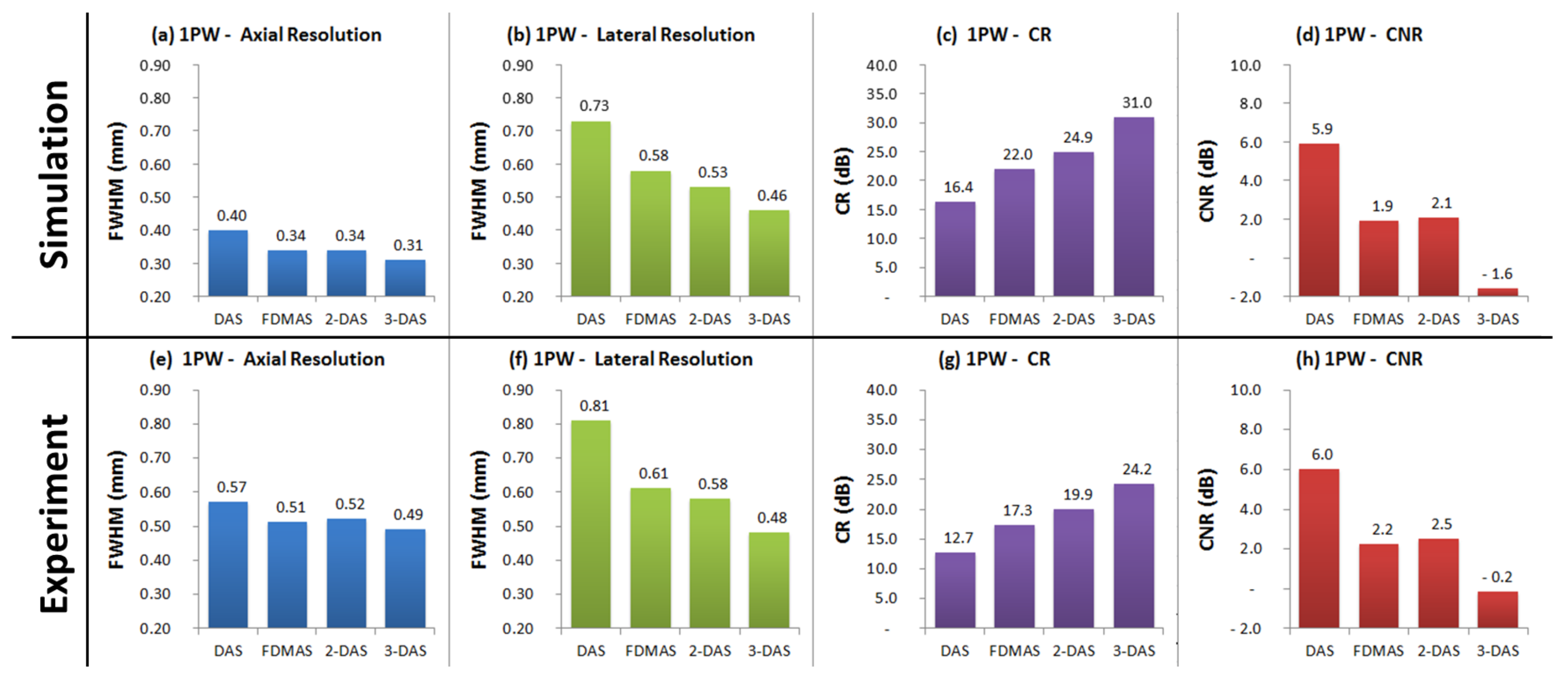
First, the results obtained for single plane wave imaging (1 PW) are considered. The images obtained on the four phantoms with 1 PW are shown in Figure 2. The measurements are summed in Figure 4. As a first observation, the resolution is enhanced with p-DAS, due to its better rejection of ill-rephased wave fronts: in Figure 4, as p increases, improved sensitivity in the lateral direction is highlighted, both in simulation (Figure 4b; DAS, 0.73 mm; 2-DAS, 0.53 mm; 3-DAS, 0.46 mm) and experiment (Figure 4f; DAS, 0.81 mm; 2-DAS, 0.58 mm; 3-DAS, 0.48 mm).
The mean axial FWHM over the 20 targets relies mainly on the excitation waveform, and it is slightly decreased for and (Figure 4a,e). For the simulated phantom (Figure 2a,c), the 20 axial FWHM are quasi constant for all of the scatterers with DAS (0.39–0.41 mm), but they decrease for the interfering scatterers when using 2-DAS (0.31–0.41 mm). The target that is most affected by interference located at ( mm, mm) has an axial FWHM of 0.40 mm with DAS, whereas this is 0.31 mm with 2-DAS. However, the FWHM of the isolated scatterer placed at ( mm, mm) is 0.40 mm for DAS and 2-DAS. Indeed, the rejection of interference for p-DAS is nonlinear with respect to amplitude, as seen for Equation (12). Then, the same interference noise is not rejected in the same way whether it interferes with the top of the pulse, or with the low-amplitude edges of the pulse. Finally, p-DAS tends to shrink the axial FWHM in the presence of interference.
In addition, the results demonstrate that the CR increases with the p-value for both simulation (Figure 4c; DAS, 16.4 dB; 2-DAS, 24.9 dB; 3-DAS, 31.0 dB) and experiment (Figure 4g; DAS, 12.7 dB; 2-DAS, 19.9 dB; 3-DAS, 24.2 dB). These observations confirm the conclusions of Section 3.1: the higher the p-value is, the more rejected the side-lobes are. As a result, the artifacts from the bright speckle into the dark cysts are attenuated for (Figure 2g,o), and even more so for (Figure 2h,p), with respect to those for DAS (Figure 2e,m).
Conversely, the CNR decreases as the p-value increases, both for simulation (Figure 4d; DAS, 5.9 dB; 2-DAS, 2.1 dB; 3-DAS, −1.6 dB) and experiment (Figure 4h; DAS, 6.0 dB; 2-DAS, 2.5 dB; 3-DAS, −0.2 dB). This means that the variance of the pixel intensities inside the cysts and inside the speckle is stronger with and even more with . Looking at the simulated images, the speckle obtained with DAS (Figure 2e,m) is relatively homogeneous with gray pixels, whereas for (Figure 2g,o) and (Figure 2h,p) the speckle is more heterogeneous, with a background that is darker. Indeed, the coherent bright spots in the speckle are not strongly impacted by p-DAS, whereas the incoherent dark pixels of the speckle are heavily rejected. As a result, the CNR drops for high p-values because it varies in the opposite way to the increased variance. The same trend is obtained for the experiment (Figure 2m,o,p).
Moreover, roughly coherent wave fronts back-scattered from point targets appear as relatively brighter spots when using or (Figure 2k,l), rather than conventional DAS (Figure 2i). Note that the energy of such high coherent targets tends to darken the speckle in their near lateral neighborhood. This phenomenon was identified by Ole et al. in [18] as an inner characteristic of beamformers based on coherence. For this reason, the p-value can be adjusted to enhance the resolution and the CR (useful for lesion detectability), while preserving the speckle structure and CNR (used for texture analysis, and so, tissue characterization) [19]. Such a trade-off was identified as common behavior for adaptive beamformers by [20].
3.2.2. Eleven Plane Wave Imaging
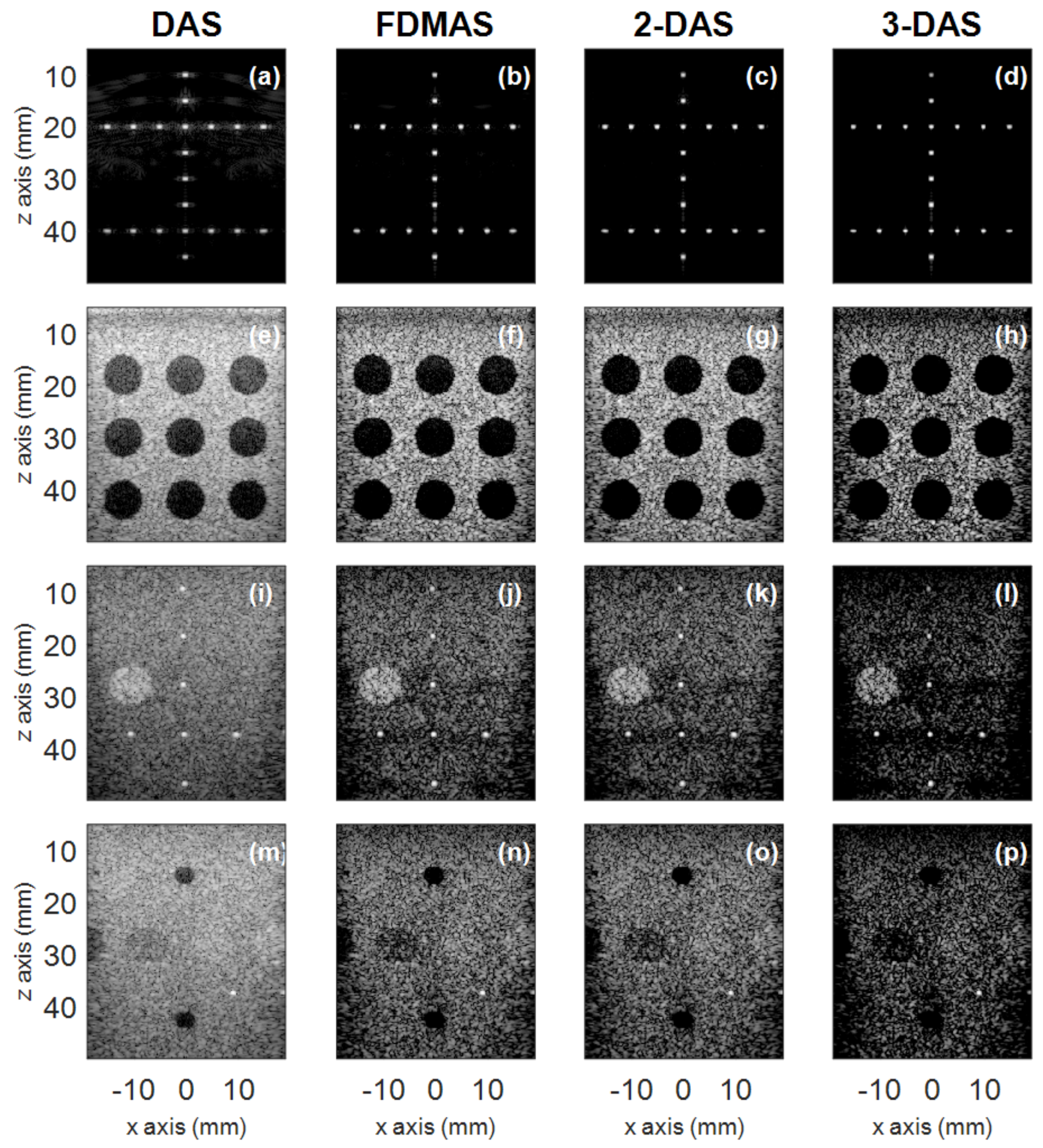
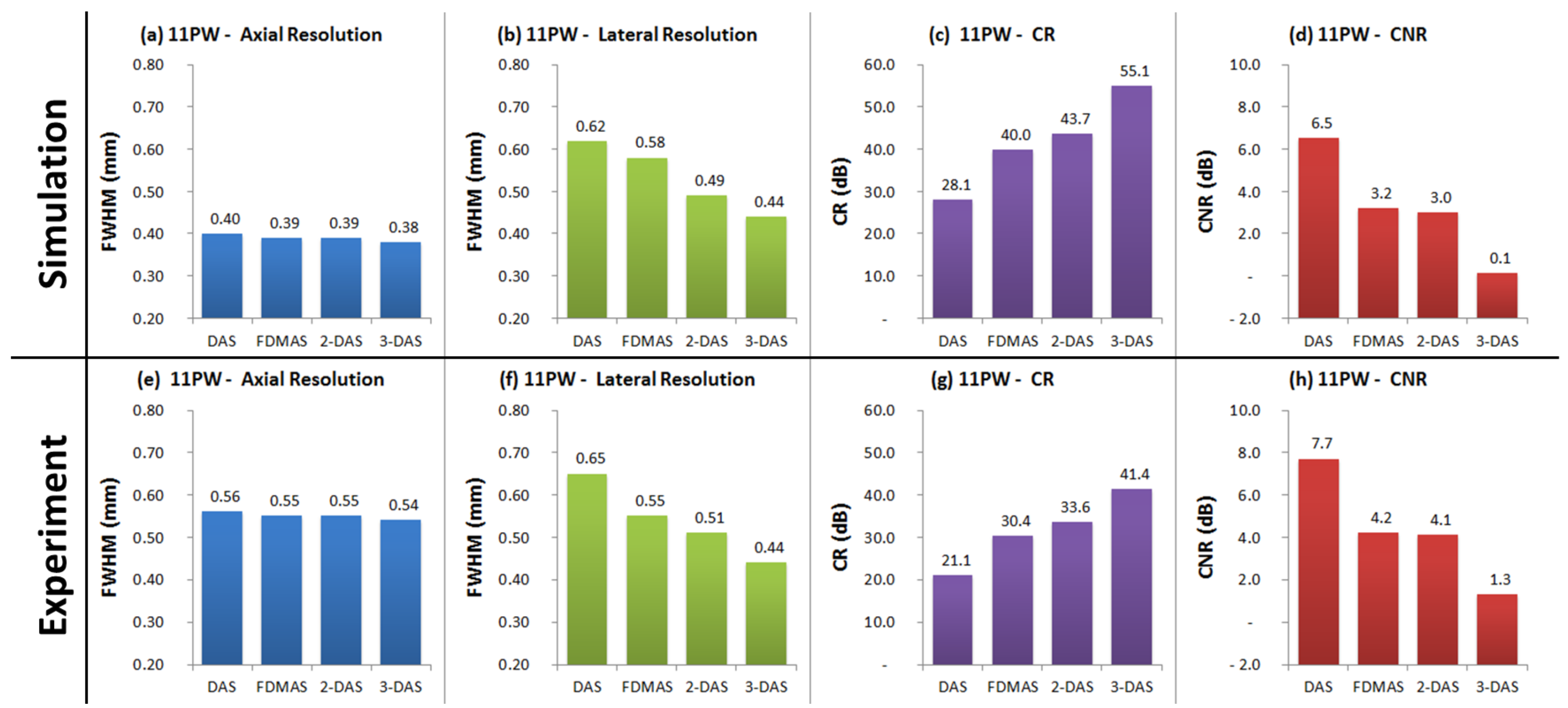
The results for 11 PW imaging are analyzed in this section. The images obtained on the four phantoms with 11 PW are shown in Figure 5. The measurements are summarized in Figure 6. The results demonstrate that p-DAS can be applied successfully to plane wave compounding since the effects of p-DAS obtained with 1 PW are preserved when using 11 PW (i.e., as p increases, better lateral resolution and CR, but worse CNR). The lateral resolution is improved as p increases both in simulation (Figure 6b; DAS, 0.62 mm; 2-DAS, 0.49 mm; 3-DAS, 0.44 mm) and experiment (Figure 6f; DAS, 0.65 mm; 2-DAS, 0.51 mm; 3-DAS, 0.44 mm). The CR is also improved for higher p-values, for both simulation (Figure 6c; DAS, 28.1 dB; 2-DAS, 43.7 dB; 3-DAS, 55.1 dB) and experiment (Figure 6g; DAS, 21.0 dB; 2-DAS, 33.6 dB; 3-DAS, 41.4 dB). In the image (Figure 5e,g,h), the cysts are darker with respect to the speckle when using or . This can be explained as follows. If the compounding leads to different mean values for each channel, this is because no coherent source is detected, but only noise or interference: the nonlinear weighting attenuates the noisy pixel value. In this way, the interferences from bright speckles in the cysts vanish, so the cysts tend to be darker, and so the CR is improved. As p-DAS increases the gap between coherent and incoherent sources, the variance inside the cyst and inside the speckle are also increased. Such darkening of the speckle structure is also noticeable on experimental phantoms (Figure 5m,o,p). In this way, the CNR decreases with the p-values for both simulation (Figure 6d; DAS, 6.5 dB; 2-DAS, 3.0 dB; 3-DAS, 0.1 dB) and experiment (Figure 6g; DAS, 7.7 dB; 2-DAS, 4.1 dB; 3-DAS, 1.3 dB). Finally, the impact of p-DAS on the axial FWHM is less than with 1 PW, for both simulation (Figure 6a; DAS, 0.40 mm; 2-DAS, 0.39 mm; 3-DAS, 0.38 mm) and experiment (Figure 6e; DAS, 0.56 mm; 2-DAS, 0.55 mm; 3-DAS, 0.54 mm). Indeed, as observed for 1 PW, the more a scatterer is impacted by interference, the more its FWHM is improved. However, as the compounding of the 11 PW before p-DAS attenuates the level of interference, the nonlinear behavior of p-DAS with respect to the amplitude is less highlighted.
In summary, p-DAS is an interesting beamformer to reject any incoherent pixel values that result from either ill rephased wavefronts, or waveforms corrupted by interference or noise. This explains the better lateral resolution and enhanced side-lobe rejection, and so the improved contrast ratio. These three first metrics increase with the p-value. However, the CNR is degraded, as the speckle results from interference, and so it is heavily rejected with respect to the coherent target. Finally, p-DAS appears to be a good candidate to resolve particularly punctual targets embedded in speckle or noise.
3.3. Comparison between FDMAS and p-DAS
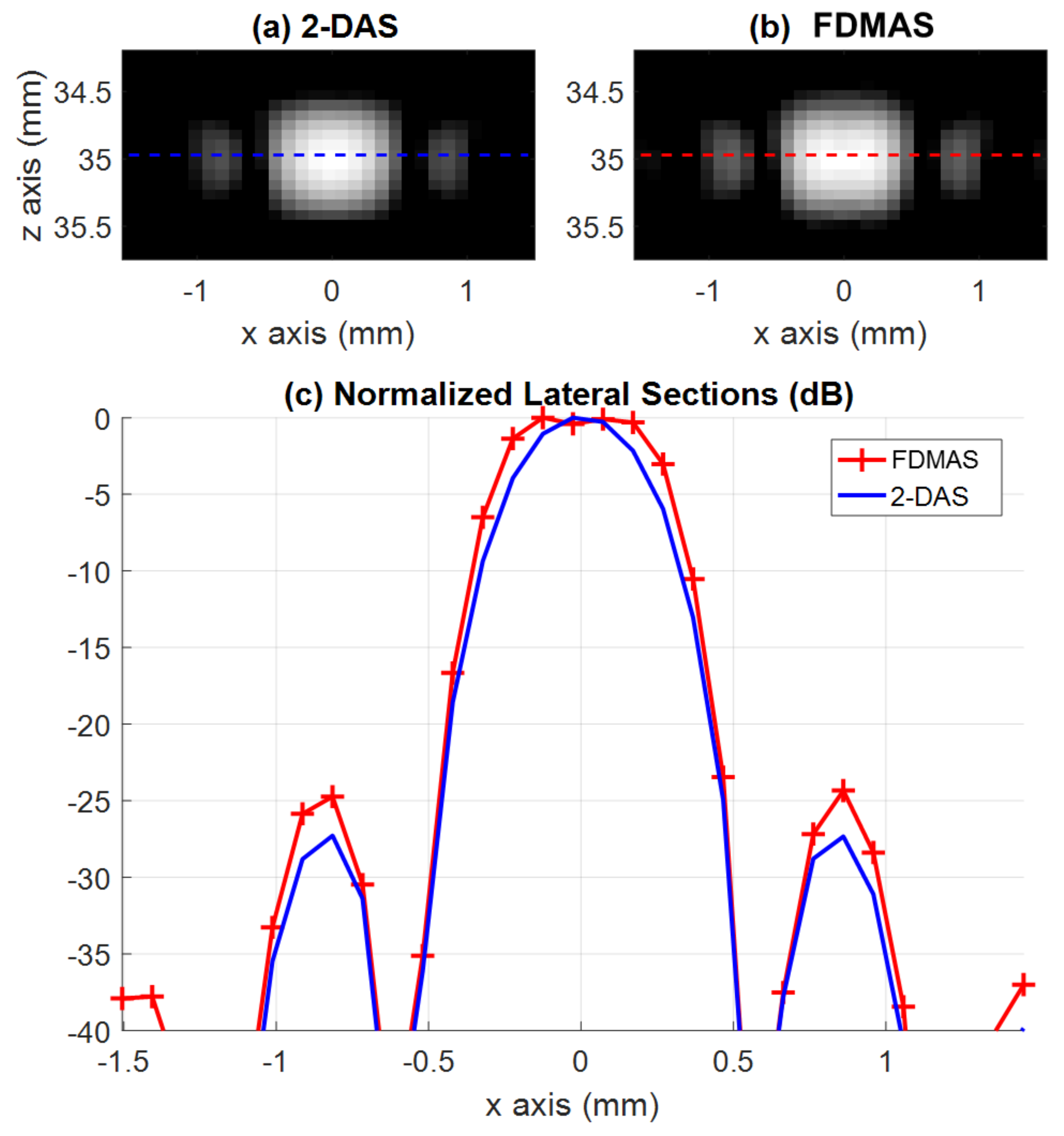
The comparison between 2-DAS and FDMAS is seen through the results obtained with single plane wave imaging. First, the images obtained with a single plane wave on the numerical phantom are compared (see Figure 2b,c). Namely, the PSFs obtained with 2-DAS and FDMAS (Figure 7a,b) are compared for the point scatterer placed at ( mm, mm). Their normalized lateral sections are plotted in Figure 7c. As a first observation, the main lobe is not flat any more when using 2-DAS beamforming rather than FDMAS beamforming. This explains the better lateral resolution for 2-DAS with respect to FDMAS (Figure 4b; 2-DAS, 0.53 mm; FDMAS, 0.58 mm). This enhancement is also seen in the experiment (Figure 4f; 2-DAS, 0.58 mm; FDMAS, 0.61 mm). Moreover, the relative enhanced side-lobe rejection of 2 dB observed for PSFs in Figure 7c leads to slightly better CR for 2-DAS than for FDMAS, for both simulation (Figure 4c; 2-DAS, 24.9 dB; FDMAS, 22.0 dB) and experiment (Figure 4g; 2-DAS, 19.9 dB; FDMAS, 17.3 dB). To explain these better performances, the role of the ‘signed’ p-power in p-DAS rather than the ’unsigned’ p-power is highlighted. A previous study by [14] demonstrated that images obtained with 2-DAS with unsigned p-power or with FDMAS are equivalent. Indeed, considering Equation (10) with the unsigned p-power with leads to:
Then, the rearranged algebraic expression of Equation (15) gives:
Finally, FDMAS expression is recovered in Equation (16), where the term (b) is negligible compared to the term (c). Indeed, when these originate from the same wave front, the have almost the same amplitudes, whatever the index n. This means that, in Equation (16), and are particularly close values. For Equation (16), as there are only N terms in the sum (b) but in the sum (c), the sum (b) can be neglected, and then is approximatively equal to . Note that a band-pass filter centred at for the RF images is necessary when using 2-DAS with the unsigned p-power, as the sign information is lost and thus the frequency content is split between the DC component and . However, using p-DAS (i.e., with the signed p-power) preserves the sign of the oscillations, and thus avoids splitting the frequency content of RF images. In this way, the band-pass filter selects the entire information maintained at , instead of just keeping the reduced part split at , as for FDMAS.
In summary, compared to FDMAS, 2-DAS avoids the flatenning of the main lobe and allows a slight better side-lobe rejection of 2 dB (Figure 7), which is consistent with the slight improved lateral resolutions and contrast ratios on the different numerical and experimental phantoms. Moreover, with the generalized formalism of p-DAS, the proposed beamformer can be tuned with the p-value to adjust the trade-off between the CR and the CNR. Finally, 2-DAS has a similar formulation as the real-time implementation of FDMAS proposed by Ramalli et al. [21].
4. Conclusions
This paper proposes a nonlinear beamformer, p-DAS, to enhance image quality. This beamformer is tested here in simulation and also under experimental conditions in the context of ultrafast plane wave imaging. The main benefits of this method are to improve lateral resolution, to better reject side lobes, and, as a consequence, to improve the contrast ratio, depending on the p-value used. However, p-DAS tends to distort the speckle statistics as the nonlinear operations increase the gap between the coherent and incoherent targets that compose the speckle, which leads to decreased CNR.
Another interesting aspect is that the proposed method is an extended version of an already well-known nonlinear beamformer: FDMAS. The signed p-power allows the removal of the PSF flat main lobe in FDMAS and better side-lobe rejection. Finally, the p-value can be tuned to find the best trade-off between CR and CNR, as required by the user.
Several applications are expected for this p-DAS beamforming. First, as p-DAS highlights punctual targets in noisy environments, it appears to be a very promising tool for bubble localization. For instance, Errico et al. reconstructed high-resolution vascular maps using ultrafast imaging of microbubbles [22]. The efficiency of the method relied on the assumption that the bubbles are punctual and separable sources, and then on the detection of a large number of them in B-mode images. p-DAS also represents a solution to increase the number of detected bubbles, as when the echo signals are weak due to ultrasound attenuation (e.g., deep tissues, through the skull, high frequency ultrasound). Another application might be imaging of cavitation for therapeutic monitoring. In [23], Boulos et al. proposed enhancing the resolution of passive imaging of cavitation with the adaptive phase coherence factor based beamformer [10]. p-DAS might also be an appropriate tool to reject interference between the punctual bubbles that compose the cavitation cloud, which generate strong artifacts on cavitation maps. Moreover, the performance of p-DAS might be investigated with other high frame rate imaging strategies. In the case of multi-line transmit [4,12], p-DAS might be a good candidate to reject the cross-talk for reception.
For the methodology, further studies can be conducted on the function used to compress the adaptive weights. Indeed, the coupling of ‘-root and p-power’ has been used in this paper, while it might be interesting to use other couplings of functions, such as ‘exponential and logarithm’, to understand their impact on image quality.
Acknowledgments
The authors would like to thank Giulia Matrone and Alessandro Stuart Savoia for their valuable discussions, and for sharing their experience of FDMAS. This work was supported by LABEX CELYA (ANR-10-LABX-0060) and was performed within the framework of the LABEX PRIMES (ANR-11-LABX-0063) of the Université de Lyon, within the programme ’Investissements d’Avenir’ (ANR-11-IDEX-0007), operated by the French National Research Agency (ANR).
Author Contributions
Maxime Polichetti, François Varray and Barbara Nicolas developed the methodology, analyzed the data, and wrote the paper. Christian Cachard and Jean-Christophe Béra are the leaders of the project, and contributed with reading and improving the manuscript.
Conflicts of Interest
The authors declare that they have no conflicts of interest.
References
- Tanter, M.; Fink, M. Ultrafast imaging in biomedical ultrasound. IEEE Trans. Ultrason. Ferroelectr. Freq. Control 2014, 61, 102–119. [Google Scholar] [CrossRef] [PubMed]
- Petrusca, L.; Varray, F.; Souchon, R.; Bernard, A.; Chapelon, J.Y.; Liebgott, H.; N’Djin, W.A.; Viallon, M. Fast Volumetric Ultrasound B-Mode and Doppler Imaging with a New High-Channels Density Platform for Advanced 4D Cardiac Imaging/Therapy. Appl. Sci. 2018, 8, 200. [Google Scholar] [CrossRef]
- Tong, L.; Gao, H.; Choi, H.F.; D’hooge, J. Comparison of conventional parallel beamforming with plane wave and diverging wave imaging for cardiac applications: A simulation study. IEEE Trans. Ultrason. Ferroelectr. Freq. Control 2012, 59, 1654–1663. [Google Scholar] [CrossRef] [PubMed]
- Tong, L.; Gao, H.; D’hooge, J. Multi-transmit beam forming for fast cardiac imaging-a simulation study. IEEE Trans. Ultrason. Ferroelectr. Freq. Control 2013, 60, 1719–1731. [Google Scholar] [CrossRef] [PubMed]
- Montaldo, G.; Tanter, M.; Bercoff, J.; Benech, N.; Fink, M. Coherent plane-wave compounding for very high frame rate ultrasonography and transient elastography. IEEE Trans. Ultrason. Ferroelectr. Freq. Control 2009, 56, 489–506. [Google Scholar] [CrossRef] [PubMed]
- Synnevag, J.; Austeng, A.; Holm, S. Adaptive beamforming applied to medical ultrasound imaging. IEEE Trans. Ultrason. Ferroelectr. Freq. Control 2007, 54, 1606. [Google Scholar] [CrossRef] [PubMed] [Green Version]
- Holfort, I.K.; Gran, F.; Jensen, J.A. Broadband minimum variance beamforming for ultrasound imaging. IEEE Trans. Ultrason. Ferroelectr. Freq. Control 2009, 56, 314–325. [Google Scholar] [CrossRef] [PubMed] [Green Version]
- Synnevag, J.F.; Austeng, A.; Holm, S. A low-complexity data-dependent beamformer. IEEE Trans. Ultrason. Ferroelectr. Freq. Control 2011, 58, 281–289. [Google Scholar] [CrossRef] [PubMed]
- Li, P.C.; Li, M.L. Adaptive imaging using the generalized coherence factor. IEEE Trans. Ultrason. Ferroelectr. Freq. Control 2003, 50, 128–141. [Google Scholar] [PubMed]
- Camacho, J.; Parrilla, M.; Fritsch, C. Phase coherence imaging. IEEE Trans. Ultrason. Ferroelectr. Freq. Control 2009, 56. [Google Scholar] [CrossRef] [PubMed]
- Matrone, G.; Savoia, A.S.; Caliano, G.; Magenes, G. The delay multiply and sum beamforming algorithm in ultrasound B-mode medical imaging. IEEE Trans. Med. Imaging 2015, 34, 940–949. [Google Scholar] [CrossRef] [PubMed]
- Matrone, G.; Ramalli, A.; Savoia, A.S.; Tortoli, P.; Magenes, G. High frame-rate, high resolution ultrasound imaging with multi-line transmission and filtered-delay multiply and sum beamforming. IEEE Trans. Med. Imaging 2017, 36, 478–486. [Google Scholar] [CrossRef] [PubMed]
- Prieur, F.; Rindal, O.M.H.; Holm, S.; Austeng, A. Influence of the Delay-Multiply-And-Sum beamformer on the ultrasound image amplitude. In Proceedings of the 2017 IEEE International Ultrasonics Symposium (IUS), Washington, DC, USA, 6–9 September 2017. [Google Scholar]
- Polichetti, M.; Varray, F.; Matrone, G.; Savoia, A.S.; Béra, J.C.; Cachard, C.; Nicolas, B. A computationally efficient nonlinear beamformer based on p-th root signal compression for enhanced ultrasound B-mode imaging. In Proceedings of the 2017 IEEE International Ultrasonics Symposium (IUS), Washington, DC, USA, 6–9 September 2017. [Google Scholar]
- Liebgott, H.; Rodriguez-Molares, A.; Cervenansky, F.; Jensen, J.A.; Bernard, O. Plane-wave imaging challenge in medical ultrasound. In Proceedings of the 2016 IEEE International Ultrasonics Symposium (IUS), Tours, France, 18–21 September 2016. [Google Scholar]
- Matrone, G.; Savoia, A.S.; Magenes, G. Filtered Delay Multiply And Sum beamforming in plane-wave ultrasound imaging: Tests on simulated and experimental data. In Proceedings of the 2016 IEEE International Ultrasonics Symposium (IUS), Tours, France, 18–21 September 2016. [Google Scholar]
- Varray, F.; Bernard, O.; Assou, S.; Cachard, C.; Vray, D. Hybrid strategy to simulate 3D nonlinear radio-frequency ultrasound using a variant spatial PSF. IIEEE Trans. Ultrason. Ferroelectr. Freq. Control 2016, 63, 1390–1398. [Google Scholar] [CrossRef] [PubMed]
- Rindal, O.M.H.; Rodriguez-Molares, A.; Austeng, A. The dark region artifact in adaptive ultrasound beamforming. In Proceedings of the 2017 IEEE International Ultrasonics Symposium (IUS), Washington, DC, USA, 6–9 September 2017. [Google Scholar]
- Thijssen, J.M. Ultrasonic speckle formation, analysis and processing applied to tissue characterization. Pattern Recognit. Lett. 2003, 24, 659–675. [Google Scholar] [CrossRef]
- Hverven, S.M.; Rindal, O.M.H.; Rodriguez-Molares, A.; Austeng, A. The influence of speckle statistics on contrast metrics in ultrasound imaging. In Proceedings of the 2017 IEEE International Ultrasonics Symposium (IUS), Washington, DC, USA, 6–9 September 2017. [Google Scholar]
- Ramalli, A.; Scaringella, M.; Matrone, G.; Dallai, A.; Boni, E.; Savoia, A.S.; Bassi, L.; Hine, G.E.; Tortoli, P. High dynamic range ultrasound imaging with real-time filtered-delay multiply and sum beamforming. In Proceedings of the 2017 IEEE International Ultrasonics Symposium (IUS), Washington, DC, USA, 6–9 September 2017. [Google Scholar]
- Errico, C.; Pierre, J.; Pezet, S.; Desailly, Y.; Lenkei, Z.; Couture, O.; Tanter, M. Ultrafast ultrasound localization microscopy for deep super-resolution vascular imaging. Nature 2015, 527, 499–502. [Google Scholar] [CrossRef] [PubMed]
- Boulos, P.; Varray, F.; Poizat, A.; Kalkhoran, M.A.; Gilles, B.; Bera, J.; Cachard, C. Passive cavitation imaging using different advanced beamforming methods. In Proceedings of the 2016 IEEE International Ultrasonics Symposium (IUS), Tours, France, 18–21 September 2016. [Google Scholar]
Figure 1.
Block diagram describing how the value of a pixel is obtained from the raw echo signals recorded after M plane wave transmissions, using the N channels of the probe. Once all the pixel values have been computed in this way, a band-pass filter (not represented here) centered at is applied along the z-dimension of the complete image, in order to remove potential artificial harmonics due to nonlinear operations.

Figure 2.
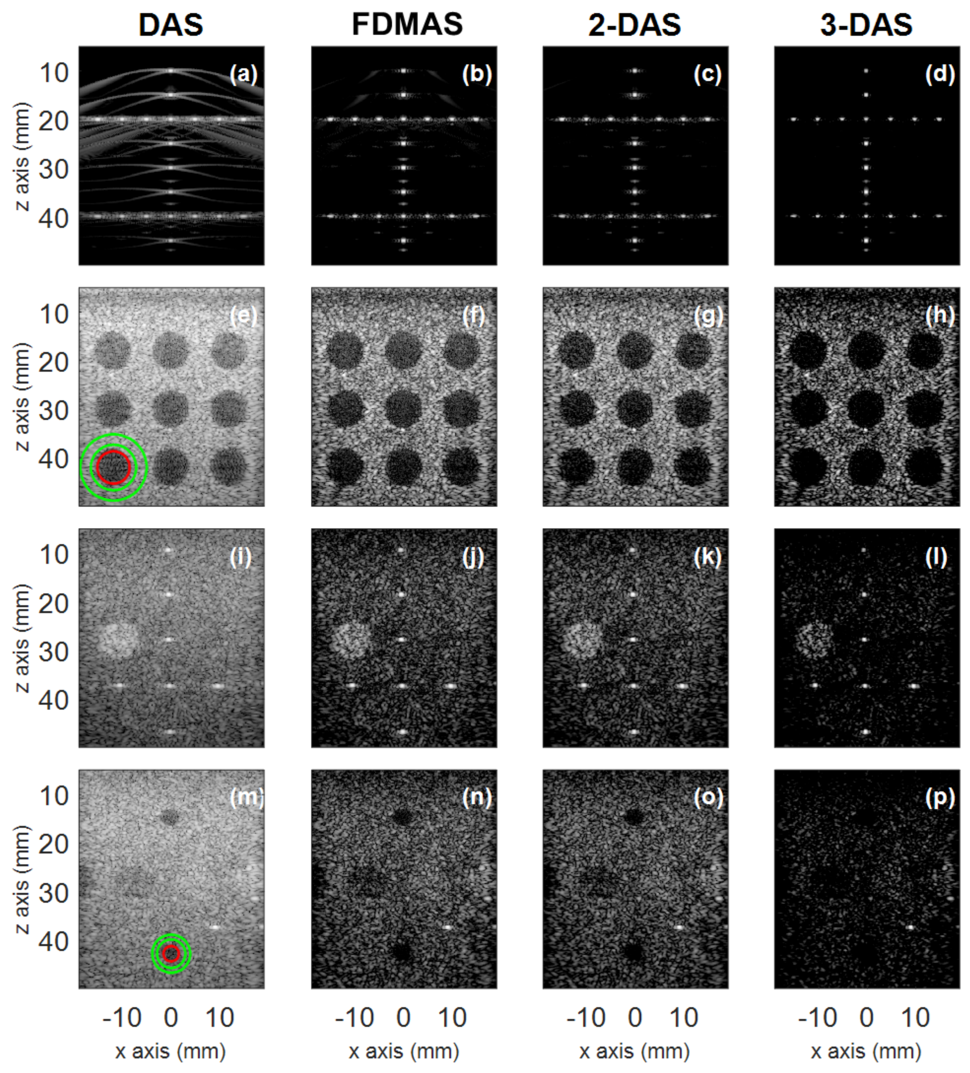
B-mode images obtained with single plane wave imaging for the four phantoms and the four beamformers compared: DAS (a,e,i,m), FDMAS (b,f,j,n), 2-DAS (c,g,k,o), and 3-DAS (d,h,l,p). (a–d) the numerical phantom used for the resolution; (e–h) the numerical phantom used for the contrast; (i–l) the experimental phantom used for the resolution; and (m–p) the experimental phantom used for the contrast. All of the images are displayed with a 60-dB dynamic range. An example of the boundaries chosen for the contrast metrics is given for simulation (e) and experiment (m), with the inside of the cyst in red, and the outside of the speckle ring in green.
Figure 2.
B-mode images obtained with single plane wave imaging for the four phantoms and the four beamformers compared: DAS (a,e,i,m), FDMAS (b,f,j,n), 2-DAS (c,g,k,o), and 3-DAS (d,h,l,p). (a–d) the numerical phantom used for the resolution; (e–h) the numerical phantom used for the contrast; (i–l) the experimental phantom used for the resolution; and (m–p) the experimental phantom used for the contrast. All of the images are displayed with a 60-dB dynamic range. An example of the boundaries chosen for the contrast metrics is given for simulation (e) and experiment (m), with the inside of the cyst in red, and the outside of the speckle ring in green.

Figure 3.
Illustration of the enhanced side-lobe rejection for the point spread function (PSF) with the proposed method with (2-DAS), compared with conventional DAS. The scatterer placed at ( mm, mm) on the numerical phantom is considered. The B-mode log-compressed images with a 40-dB dynamic range are shown for DAS (a) and 2-DAS (b). The delayed signals are shown for mm (c) and mm (d); (e) the delayed samples for the pixel on the main lobe are shown in blue, with their corresponding adaptive weights in red; and (f) the delayed samples for the pixel on the side lobe are shown in blue, with their corresponding adaptive weights in red.

Figure 4.
Performances obtained with DAS, FDMAS, 2-DAS, and 3-DAS beamformers, using a single plane wave in simulations (a–d) and experiments (e–h). The results obtained are given for axial resolution (a,e), lateral resolution (b,f), contrast ratio (c,g), and contrast-to-noise ratio (d,h).
Figure 4.
Performances obtained with DAS, FDMAS, 2-DAS, and 3-DAS beamformers, using a single plane wave in simulations (a–d) and experiments (e–h). The results obtained are given for axial resolution (a,e), lateral resolution (b,f), contrast ratio (c,g), and contrast-to-noise ratio (d,h).

Figure 5.
B-mode images obtained with eleven plane wave imaging for the four phantoms and the four beamformers compared: DAS (a,e,i,m), FDMAS (b,f,j,n), 2-DAS (c,g,k,o), and 3-DAS (d,h,l,p). (a–d) the numerical phantom used for the resolution; (e–h) the numerical phantom used for the contrast; (i–l) the experimental phantom used for the resolution; and (m–p) the experimental phantom used for the contrast. All of the images are displayed with 60-dB dynamic range.

Figure 6.
Performances obtained with DAS, FDMAS, 2-DAS, and 3-DAS beamformers, using 11 plane waves in simulation (a–d) and experiment (e–h). Results obtained are given for axial resolution (a,e), lateral resolution (b,f), contrast ratio (c,g), and contrast-to-noise ratio (d,h).
Figure 6.
Performances obtained with DAS, FDMAS, 2-DAS, and 3-DAS beamformers, using 11 plane waves in simulation (a–d) and experiment (e–h). Results obtained are given for axial resolution (a,e), lateral resolution (b,f), contrast ratio (c,g), and contrast-to-noise ratio (d,h).

Figure 7.
Comparison of PSFs obtained with 2-DAS and FDMAS. The scatterer was placed at ( mm, mm) on the numerical phantom. B-mode log-compressed images are shown over a 40-dB dynamic range for 2-DAS (a) and FDMAS (b). Their respective normalized lateral profiles are shown in (c).
Figure 7.
Comparison of PSFs obtained with 2-DAS and FDMAS. The scatterer was placed at ( mm, mm) on the numerical phantom. B-mode log-compressed images are shown over a 40-dB dynamic range for 2-DAS (a) and FDMAS (b). Their respective normalized lateral profiles are shown in (c).


Table 1.
Transmission settings for the PICMUS challenge [15].
Table 1.
Transmission settings for the PICMUS challenge [15].
| Number of Elements N | 128 | Excitation (number of cycles) | 2.5 |
| Pitch (mm) | 0.3 | Transmit frequency (MHz) | 5.2 |
| Element width (mm) | 0.27 | Sampling Frequency (MHz) | 20.8 |
© 2018 by the authors. Licensee MDPI, Basel, Switzerland. This article is an open access article distributed under the terms and conditions of the Creative Commons Attribution (CC BY) license (http://creativecommons.org/licenses/by/4.0/).
Share and Cite
MDPI and ACS Style
Polichetti, M.; Varray, F.; Béra, J.-C.; Cachard, C.; Nicolas, B. A Nonlinear Beamformer Based on p-th Root Compression—Application to Plane Wave Ultrasound Imaging. Appl. Sci. 2018, 8, 599. https://doi.org/10.3390/app8040599
AMA Style
Polichetti M, Varray F, Béra J-C, Cachard C, Nicolas B. A Nonlinear Beamformer Based on p-th Root Compression—Application to Plane Wave Ultrasound Imaging. Applied Sciences. 2018; 8(4):599. https://doi.org/10.3390/app8040599
Chicago/Turabian StylePolichetti, Maxime, François Varray, Jean-Christophe Béra, Christian Cachard, and Barbara Nicolas. 2018. "A Nonlinear Beamformer Based on p-th Root Compression—Application to Plane Wave Ultrasound Imaging" Applied Sciences 8, no. 4: 599. https://doi.org/10.3390/app8040599
Note that from the first issue of 2016, this journal uses article numbers instead of page numbers. See further details here.