Matched-Filter Thermography

Department of Mechanical Engineering, York University, 4700 Keele Street, Toronto, ON M3J 1P3, Canada
Appl. Sci. 2018, 8(4), 581; https://doi.org/10.3390/app8040581
Submission received: 31 January 2018
/
Revised: 26 March 2018
/
Accepted: 4 April 2018
/
Published: 8 April 2018
(This article belongs to the Special Issue Recent Advances and Applications of Infrared Thermography)
Abstract
:Conventional infrared thermography techniques, including pulsed and lock-in thermography, have shown great potential for non-destructive evaluation of broad spectrum of materials, spanning from metals to polymers to biological tissues. However, performance of these techniques is often limited due to the diffuse nature of thermal wave fields, resulting in an inherent compromise between inspection depth and depth resolution. Recently, matched-filter thermography has been introduced as a means for overcoming this classic limitation to enable depth-resolved subsurface thermal imaging and improving axial/depth resolution. This paper reviews the basic principles and experimental results of matched-filter thermography: first, mathematical and signal processing concepts related to matched-fileting and pulse compression are discussed. Next, theoretical modeling of thermal-wave responses to matched-filter thermography using two categories of pulse compression techniques (linear frequency modulation and binary phase coding) are reviewed. Key experimental results from literature demonstrating the maintenance of axial resolution while inspecting deep into opaque and turbid media are also presented and discussed. Finally, the concept of thermal coherence tomography for deconvolution of thermal responses of axially superposed sources and creation of depth-selective images in a diffusion-wave field is reviewed.
1. Introduction
Active thermography is a rapidly growing non-destructive testing (NDT) technique, which, since the 1980s [1], has been widely employed in research settings for detection of defects in a broad range of materials. The principle behind active thermography is quite straightforward: the sample is exposed to some form of excitation to create a thermal-wave field inside sample while the surface temperature is constantly registered by an infrared camera. The presence of defects causes perturbation in the thermal-wave field; such perturbations are used as indications of the presence of defects. Depending on the waveform shape of excitation (pulse vs. intensity-modulated) and the signal processing scheme used, active thermography branches into two major streams of Pulsed Thermography (PT) and Lock-In Thermography (LIT). Both techniques are specifically popular for inspection of industrial samples. For instance, they have been widely used for detection of damage in Carbon Fiber Reinforced Plastic (CFRP) materials [2], inspection of airplane parts [3] and detection of leakages in integrated circuits [4]. More recently, active thermography has been utilized in biomedical applications such as detection of malignancies in human soft [5,6] and hard tissues [7,8,9,10,11] as well as sensitive interpretation of lateral flow immunoassays [12]. Specifically, detection of dental caries at very early stages of formation has proven to be a key application of thermography in biomedicine by providing diagnostic contrast based on enhanced absorption of light at caries [7,8,9], as opposed to other emerging technologies such as Raman spectroscopy [13] and optical coherence tomography (OCT) [14,15], which rely on changes in scattering of light at caries. Appealing, if not unique, characteristics of thermography include: being no-contact, having the ability to inspect opaque [4,16,17,18,19,20] and turbid materials [7,8,9], and being scalable [3,4]. Moreover, depending on the application, different types of external excitation, such as optical [7], magnetic [17], mechanical waves [19], electrical [4,16] or even cyclic stress/strain [18], can be utilized to induce the thermal wave field inside the sample. A comprehensive review of conventional thermography techniques such as PT and LIT can be found in another paper of this special issue on “Novel Ideas for Infrared Thermography also Applied in Integrated Approaches”.
2. Shortcoming of Conventional Active Thermography
Despite the appealing attributes, the performance of conventional active thermography techniques is limited by the diffusive nature of heat conduction. That is, an inherent compromise needs to be made between inspection depth and depth resolution. In PT, in order to inspect deep into samples, larger energy needs to be deposited into the sample. Since the maximum excitation power is often limited by availability and complexity of high power excitation sources, and also by the maximum permissible exposure of the sample, larger energy deposition can practically be achieved by increasing the duration of pulses. However, increasing pulse duration results in superposition of transient thermal responses of closely spaced defects and thus deteriorates depth resolution. LIT suffers from a similar trade-off. That is, a deep inspection into samples can be achieved at low modulation frequency due to the increase in the thermal diffusion length. However, increase in thermal diffusion length also increases the thermal wavelength and thus depreciates depth resolution. Recently, incorporation of matched-filtering in thermography has been proposed [21,22,23,24,25] for overcoming the classic compromise of conventional active thermography in order to maintain depth resolution while inspecting deep in samples. The sections below review the fundamentals of matched-filter thermography based on the works of Tabatabaei and Mandelis [21,22,23,26].
3. Matched Filtering
A matched filter (MF) is commonly defined as the optimal linear filter for maximizing the signal-to-noise ratio (SNR) in the presence of additive stochastic noise [27]. The methodology was introduced in the 1940s [28] and has since gained widespread adaptation in numerous fields such as telecommunication, radar design and medical imaging.
3.1. Idea behind the Technique
MF relies on orthogonality of harmonic functions and uses this property to detect replica(s) of a pre-known signal in noisy channels. The well-known cross-correlation (CC) technique is a special case of a MF, mathematically defined as:
where and are the pre-known signal (i.e., filter) and the noisy response containing replica(s) of the pre-known signal, respectively. Equation (1) is very similar to the mathematical definition of orthogonality of harmonic functions:
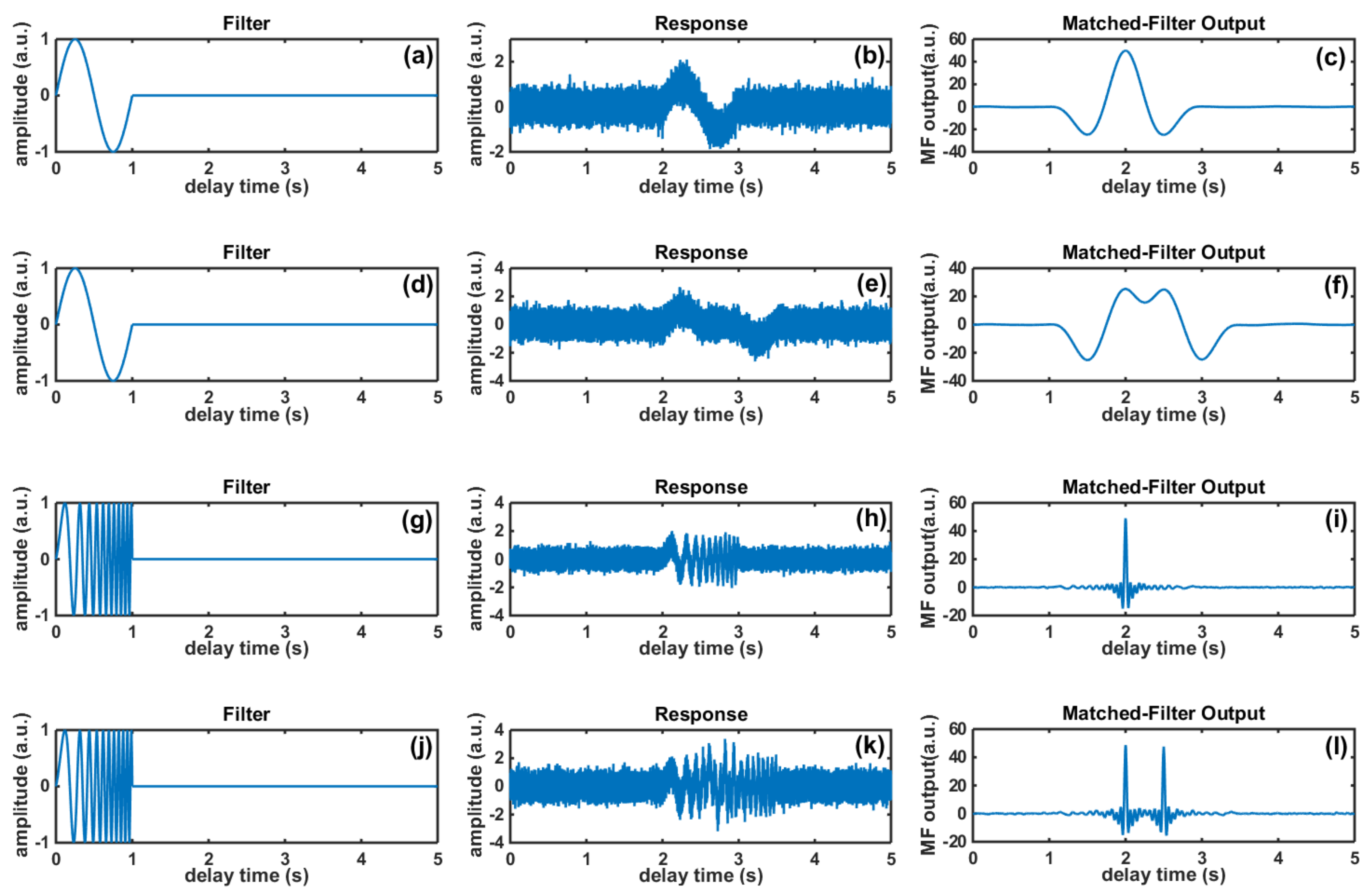
Comparison of Equations (1) and (2) implies that MF operates based on incremental delaying of response with respect to the pre-known signal/filter and examining the orthogonality of the two waveforms at any incremental delay. As such, when the filter and its replica become in-phase at a certain imposed delay time (i.e., delayed response matches the filter), the output of Equation (1) becomes a large value, but, when the delayed response does not match the filter, the output becomes small due to the orthogonality property of harmonic functions. The stochastic noise in the response will have minimal contribution to the MF output due to its nonexistence in the pre-known/filter waveform. Figure 1 depicts several plots to highlight the basic operating principles of MF. Panel (a) shows a single cycle of a 1 Hz sinusoidal signal as the pre-known waveform/filter, while panel (b) is a simulated response that is composed of a delayed version () of filter and stochastic noise (SNR = 10). As expected from mathematical representation of cross-correlation, the MF output, panel (c), contains a waveform with a single broad peak located at , indicating the delay between the filter and response. Note the minimal contribution of noise to the MF output and the significant improvement of SNR compared to the response waveform. Panels (e) and (f) depict a scenario where the response contains two delayed replicas of the filter () to highlight the motivation behind the concept of pulse compression in MF. In this scenario, the MF output is incapable of resolving the two responses, reliably, due to the superposition of the broad MF peaks of the individual responses.
3.2. Pulse Compression
Range/depth resolution can be enhanced in MF by incorporation of pulse compression techniques. That is, the pre-known signal can be coded with different types of phase or frequency compression techniques (e.g., linear frequency modulation/chirping or binary phase coding) in order to make the MF output waveform narrow. Panels (g)–(i) show a scenario in which linear frequency modulation has been implemented (chirp frequency range 1Hz to 20Hz; duration 1s) to enhance the range resolution; note the narrow output of MF in panel (i). By doing so, MFs gain the ability to simultaneously enhance both SNR and range resolution. This enhancement can be readily observed through comparison of the MF outputs of panels (c) and (i) and those from two delayed replicas of the filter (), panels (l) and (f).
3.3. Frequency Domain Interpretation of Matched Filtering
Implementation of Equation (1) in instrumentation requires allocation of sizable computation power for calculation of the cross-correlation integral. In order to avoid this complication, cross-correlation can be computed from the spectrums of filter and response (i.e, the frequency-domain interpretation of MF) as:
Here, denote Fourier transform, inverse Fourier transform and the complex conjugate operator, respectively. Implementation of Equation (3) instead of Equation (1) in instrumentation considerably improves the efficiency of computations thanks to the optimal fast Fourier transform routines available in most computational and instrumentation commercial software such as Matlab R2018a (MathWorks, Natick, MA, USA) and LabVIEW 2017 (National Instruments, Austin, TX, USA). Moreover, computation power can be drastically increased by parallel computing and performance of the Fourier transforms on graphics processing units (GPUs), for example through the readily available CUDA platform on most Nvidia (Nvidia Corporation, Santa Clara, CA, USA) GPUs.
4. Matched Filtering in Thermography
The first report of matched filtering in thermal-wave-based systems dates back to 1983 by Kirkbright et al. [29] in which cross-correlation using a pulsed matched filter was used in a photothermal radiometry setup to recover photothermal responses of individual layers in ultrathin multilayer samples. This work was complemented by a series of papers by Mandelis et al. in 1986, who reported on thermal-wave matched filtering using a continuous-wave matched filter incorporating a frequency-modulation pulse compression technique [30,31,32]. More recently, Tabatabaei and Mandelis [21,23] and Mulaveesala and Tuli [24,25] incorporated a linear frequency modulation matched filtering in thermography platforms and demonstrated the ability of thermographic matched-filter systems in maintaining range resolution while inspecting deep into samples, laying the foundation of the “Thermal-Wave Radar (TWR)” technique, which is used today by researchers for non-destructive evaluation of materials [33,34,35,36,37,38]. The concept of cross-correlation phase was introduced by Tabatabaei and Mandelis [23] in 2011 as an emissivity-normalized contrast channel in thermal-wave matched filtering, similar to that of lock-in thermography [39]. A significant breakthrough was achieved in the field by Tabatabaei and Mandelis’ introduction of thermal coherence tomography (TCT) [22,26], which used the binary phase coding pulse compression technique (i.e., a narrow-band phase encoding technique) to optimize the thermal-waves’ matched-filter responses in order to resolve overlaying absorbers in a diffusive field. Application of matched-filtering in a thermography system using pulsed excitation was first demonstrated by Kaiplavil and Mandelis [40] in 2011 and was later optimized to yield a highly depth-resolved thermal-wave tomographic imaging modality, termed truncated-correlation photothermal coherence tomography (TC-PCT) [41,42,43,44]. Some other fundamental advancements in the field of TWR include: incorporation of Barker [45] and Golay [46,47] code pulse compression techniques and performance optimization using spectral shaping [48]. Sections below review the fundamentals of TWR (i.e., frequency-modulated pulse compression) and TCT (i.e., phase-modulated pulse compression) based on the works of Tabatabaei and Mandelis [21,22,23,26]. Review of TC-PCT will be discussed in another paper of this special issue on “Novel Ideas for Infrared Thermography Also Applied in Integrated Approaches”.
4.1. Thermal-Wave Radar (TWR)
4.1.1. Theory and Modeling
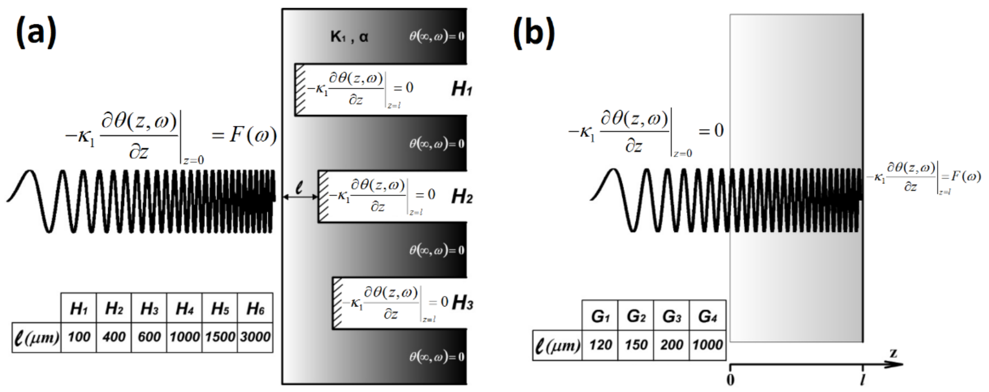
The one-dimensional thermal-wave field induced in an opaque medium of thickness , Figure 2a, by a linearly frequency modulated (LFM) optical excitation on sample surface can be mathematically modeled in frequency-domain as:
where are thermal diffusivity, thermal conductivity, the incident LFM laser beam spectrum, and sample equilibrium temperature, respectively.
Equation (4) is a homogeneous second-order ordinary differential equation that can be solved by finding the solutions of the corresponding characteristic equation and application of boundary conditions [21]. Therefore, using Planck’s law of radiation, the radiometric signals registered by the infrared camera from the surface of an opaque sample with thickness , can be found as:
where is the complex wavenumber. Similarly, the TWR response of a semi-infinite opaque material can be calculated as:
Moreover, using Equations (5) and (6), the delayed thermal contributions of subsurface defects can be isolated from the total TWR response by subtracting the response of the semi-infinite sample from that of the finite thickness sample (i.e., TWR subtraction mode):
Following a similar procedure, the TWR response of a subsurface absorber at depth in a transparent medium, Figure 2b, can be modeled and found as:
where is the average infrared absorption coefficient of transparent medium over the detection wavelength range. Therefore, by applying the frequency-domain interpretation of cross-correlation to Equations (5)–(8), the TWR/matched-filter output can be simulated for finite opaque and transparent materials as well as for semi-infinite opaque media.
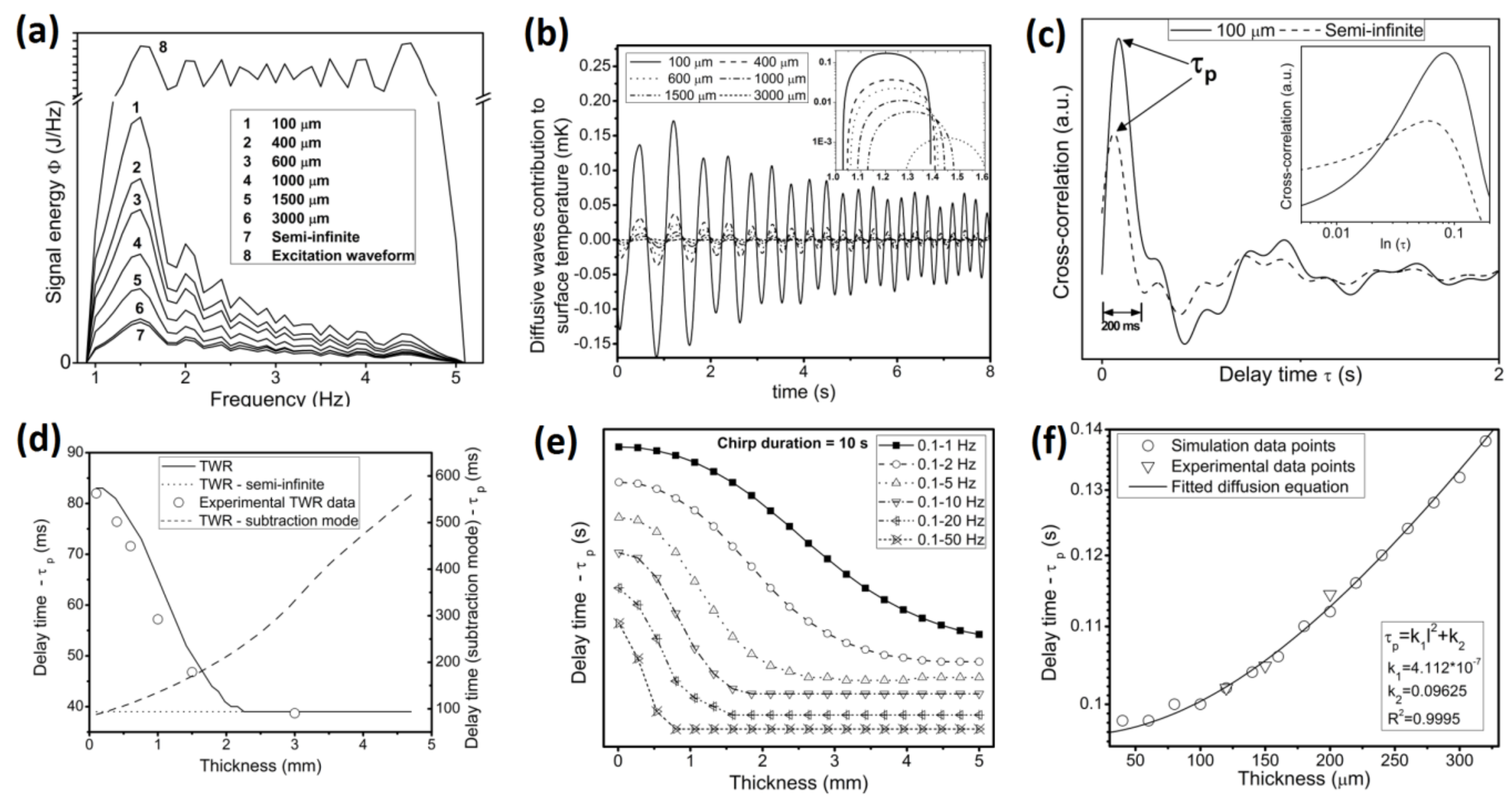
Figure 3a depicts the energy spectral density of simulated radiometric signals, Equation (5), from steel samples with various thicknesses along with the energy spectral density of the simulated radiometric signal of semi-infinite steel, Equation (6). For the purpose of comparison, the energy spectral density (ESD) of the optical excitation waveform (i.e., of the filter) is also included.
The spectral energy of the radiometric response from the steel sample surface can be divided into two parts: the energy due to excitation generated diffusive waves at the sample surface (surface energy absorption) and the coherently accumulated energy due to back-interface interacted thermal-waves. Surface energy absorption increases the sample surface temperature and therefore produces a radiometric signal whose spectral energy distribution exhibits the damped behavior expected under the envelope of diffusion (a low pass filtering action). On the other hand, the energy due to back-interface interacted thermal-waves in finitely thick opaque solids is delayed (phase-shifted) with respect to the surface absorption energy part. In a semi-infinite sample, the radiometric signal energy (Figure 3a, curve 7) is only due to surface energy absorption and no delayed back-interface interacted thermal-wave contribution is expected. As a result, a relatively uniform ESD is observed, characterized by the diffusive low-pass filtering profile (damping). The surface energy absorption part is also present in the ESD of finite thickness opaque samples. However, the interface interacted thermal-wave part of the ESD in these samples (both back and front interfaces) contribute to the resulting diffusion-wave frequency spectrum. In this sense, the delayed portion of the ESD (subtractive part) becomes a function of sample thickness and can be used as a sensitive parameter to distinguish various thicknesses, Figure 3b. Figure 3a,b suggest that, as the sample thickness decreases, the subtractive mode energy density increases. The energy increase is more pronounced at lower frequencies as low frequency components are less damped during their propagation.
Figure 3c shows the simulated TWR/cross-correlation output signals for 100 μm-thick and semi-infinite steel samples. It can be observed that, as the steel sample thickness increases from 100 μm to infinity, the cross-correlation peak delay time () decreases from 83 ms to 39 ms, as magnified in the figure inset. In addition, since the radiometric signal amplitude decreases as the sample thickness increases, the actual cross-correlation peak values are significantly different between these samples (32% difference). The theoretical TWR cross-correlation peak delay times as a function of sample thickness are plotted in Figure 3d (solid line). Simulations suggest that the TWR output peak delay time decreases as the thickness increases. This is due to the fact that increasing the sample thickness dampens the contribution of thermal-waves from depths other than the surface, such as confined thermal-waves at the steel–air back interface. As a result, the ESD of the TWR signal becomes more similar to that of the semi-infinite sample and the TWR cross-correlation peak delay time approaches that of the semi-infinite sample (dotted line), as expected. The cross-correlation peak delay time of a semi-infinite sample has a non-zero value (39 ms) due to the well-known time shift of the surface temperature oscillation with respect to the incident thermal-wave flux [49]. The dashed line in Figure 3d represents the theoretical variation of the TWR subtractive mode cross-correlation with sample thickness. This simulation suggests the capability of TWR in resolving delayed contributions from much deeper regions in the subtractive mode. It can be observed that, as the sample thickness increases, the contribution is more delayed due to the increase in thermal-wave conduction distance. Figure 3e illustrates the effect of chirp excitation parameters on the TWR output. Simulations suggest that, at a fixed starting frequency (), as frequency modulation sweep rate decreases, the theoretical detection range increases; however, at the same time, the range resolution (slope of lines) between shallow defects decreases. Therefore, the TWR chirp parameters can be tailored to the specifics of an application to yield optimal results. The simulation of TWR responses of absorbers in transparent media, Figure 3f, follows a similar pattern to that of the subtractive mode in opaque materials in that the registered cross-correlation peak delay time increases with increase in depth of the absorber, as expected.
Similar to the conventional lock-in thermography, the continuous wave nature of excitation in TWR allows for definition of phase channel. Tabatabaei et al. [23] introduced the concept of cross correlation phase to the thermal-wave sciences as an emissivity-normalized contrast parameter with enhanced sensitivity. The cross-correlation phase can be found by cross correlating the response with a pre-known signal/filter and its quadrature as:
Note how emissivity, , is cancelled out in the cross-correlation phase channel. Careful interrogation of Equations (3) and (9) indicates that cross-correlation using mono-frequency excitations (i.e., without pulse compression) leads to identical results as conventional lock-in thermography.
The abovementioned theoretical derivations and simulations suggest that four contrast parameters can be defined based on the output of TWR:
- Cross-correlation peak delay time (),
- Cross-correlation peak amplitude,
- Cross-correlation phase at ,
- Cross-correlation phase at .
4.1.2. Instrumentation
The experimental setup for matched-filter thermography can be constructed using either a single point detector or an infrared camera, Figure 4a,b, respectively. In either case, the excitation source is a continuous laser system capable of modulating the intensity of light via an analogue signal input. The sample is usually fixed on a 4 degree-of-freedom stage with its region of interest located at the focus of the infrared light collection system. An elliptic mirror can be used to feed the infrared radiation from the sample surface, located at one focal point of ellipse, to the other focal point of the mirror where the detector resides. For thermography systems, an extension tube can be used between the lens and camera’s detector array to achieve a magnification around unity. Multifunctional data acquisition devices can be used to generate three signals: detector trigger signal, flag signal, and reference/modulation signal. The detector trigger signal determines when data need to be acquired from the detector either as a point reading or acquisition of a frame. Flag pulse train determines the beginning of each modulation cycle (e.g., beginning of each linearly LFM chirp) and is used for coherent averaging of responses for improving SNR. Reference/modulation signal serves as the pre-known waveform/filter and is also responsible for modulating the intensity of light source. Research grade infrared cameras often have the ability to store the flag pulse train and reference/modulation signal information in the header of each acquired frame so that the information can later be retrieved and used in the post-acquisition signal processing.
Figure 4c depicts the block diagram of matched-filter signal processing, which can be utilized in experimental setups to carry out Equations (3) and (9) using the operators/subroutines available in common instrumentation software such as Matlab and LabView. In this diagram, represents the reference signal (i.e., pre-known waveform or filter) and represents the detector signal. For thermography systems, the signal processing algorithm is applied to the time-lapsed signal corresponding to each camera pixel.
4.1.3. Select TWR Experimental Results
One of the commonly used experimental models for characterization of photothermal radiometry systems is an opaque sample with blind holes as it mimics the presence of sharp subsurface defects at varying depths from the interrogation surface. Figure 5a,b show the results of a conventional frequency-domain photothermal radiometry (FD-PTR; analogous to lock-in thermography) carried out at 5 Hz along the centerline of holes with varying distances, , from the interrogation surface. It can be seen that the spatial scan can clearly detect the shallow subsurface holes/defects but not the deep ones. Figure 5c,d, on the other hand, depict the TWR spatial scan along the same lines as those of panels (a) and (b) using same experimental conditions used in the FD-PTR experiments (e.g., laser power, measurement time, etc.). The enhanced dynamic range of TWR can clearly be observed when comparing the performance of the two methodologies in detecting deep subsurface defects. Similar to FD-PTR, the TWR delay time can be fitted to the theoretical model, to estimate the subsurface depth of the holes (Figure 3d; solid line, and open circles, respectively).
The theoretical case of subsurface absorber at depth in a transparent medium can experimentally be modeled using back-painted glass sample of thickness . Experimental TWR results from such samples are presented in Figure 5e. For the front-surface painted glass sample, the presence of the TWR cross-correlation maximum at τ = 0 indicates pure surface absorption (no delayed conductive contribution from underlayers). For the back-surface painted glass samples, as the thickness of the glass increases, the corresponding peak delay time also increases (as predicted by theory; Figure 3f). Furthermore, with an increase in glass thickness, the TWR signal is strongly attenuated as thermal-waves decay exponentially across the glass thickness. The TWR peak delay time, , is directly linked to the depth of the absorber and as such can be fitted to the diffusive equation τp(l) = k1l2 + k2 to approximate the depth of absorbers (Figure 3f; solid line and ∇).
Figure 6 shows the TWR images from a transparent sample with two iso-depth absorbers with different light absorption coefficients. Panels (a)–(c) are the images obtained using cross correlation amplitude, peak delay time, and phase, respectively, and panels (d)–(f) show their horizontal mean profiles, respectively. It can be seen that the amplitude channel is representative of the amount of energy absorption by the two equally deep absorbers (green and black paints), yielding significantly different amplitude values. Consequently, the amplitude channel is not a true measure of the depth of the absorber. However, the peak delay time and phase values are linked to the true depth of the absorbers as they maintain the same value over the two absorbers regardless of their absorption coefficients. In terms of SNR, the amplitude channel is significantly stronger than the peak delay time and phase channels, and therefore the amplitude images should always be used to complement the information obtained from the phase and peak delay time images.
4.2. Thermal Coherence Tomography (TCT)
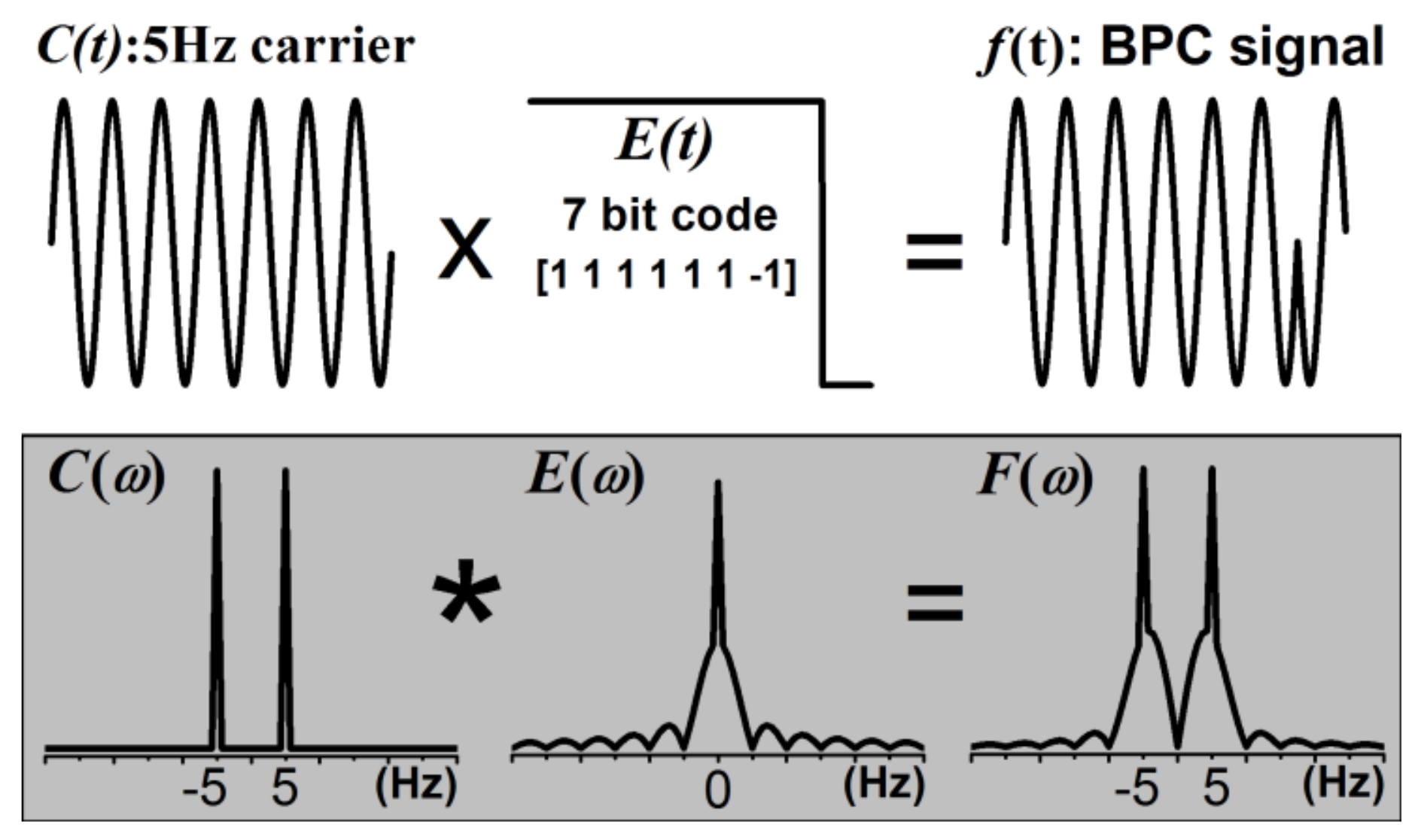
Thermal Coherence Tomography (TCT) is very similar in nature to TWR. The key differentiator of the two techniques is in the pulse compression methodology. That is, TWR incorporates a wideband LFM scheme for pulse compression while TCT uses a narrowband phase modulation scheme known as binary phase coding (BPC) [50]. The BPC signal consists of a single frequency carrier and a binary coded envelope. The narrowband signal is formed either by multiplying these components in the time-domain or alternatively by convolving their spectra in the frequency-domain (Figure 7).
4.2.1. Theory and Modeling
Detailed derivations for analytical expression of a BPC signal and TCT responses of absorbers in turbid media are provided by Tabatabaei and Mandelis in their 2011 publication in the journal of Physical Review Letters [22]. Briefly, the TCT response of absorbers in turbid media can mathematically be modelled as:
where is the local fluence of optical excitation at depth . Note the similarity of the thermal-wave field equation in the frequency-domain to the Helmholtz equation of hyperbolic wave-fields. Equation (10) is an ordinary non-homogenous differential equation system whose solution can be found as superposition of the homogeneous and particular solutions [22]. Figure 8a plots the theoretical CC phase of two extreme cases for a 7-bit binary code as a function of the subsurface absorber depth, , at several carrier frequencies. In both cases, at a given carrier frequency, the deeper the absorber, the larger the amount of phase shift, showing a more delayed contribution from the deeper absorber. Moreover, an increase in the carrier frequency reduces the maximum probing depth due to the reduced thermal diffusion length, as expected. The key point in this figure is the effect of . The infrared radiation captured by the detector is composed of a delayed conductive thermal-wave portion and an instantaneous direct Planck emission. While an increase in the direct emission improves the signal-to-noise ratio of the amplitude channel, it deteriorates the maximum probing depth of the phase channel. This occurs because the direct emissions from absorbers at different depths are instantaneous and therefore all in phase, dominating the depth-dependent phase information of the conductive portion and consequently limiting the maximum probing depth, as observed in Figure 8a.
Figure 8b shows how the height (peak amplitude channel) and location (peak delay time channel) of the CC signal peak behave as a function of the absorber depth at various carrier frequencies. Generally, a shallower absorber results in a higher amplitude and shifts the CC peak location to shorter delay times to manifest a less attenuated thermal-wave source closer to the interrogated surface. In other words, matched-filtering localizes the energy of the long-duty BPC excitation under a narrow peak whose location on the delay time axis is linked to the depth of the source and allows one to construct iso-delay images. As such, TCT can be considered as the diffusion equivalent of optical coherence tomography (OCT). Moreover, while the amplitude channel has by far the highest SNR, its reliability depends on the illumination and sample surface conditions because, unlike phase and peak delay time, it is not an emissivity normalized quantity. Another interesting feature of TCT imaging is the effect of code length. While increasing the code length does not alter the CC phase and peak delay time curves of Figure 8, it increases the pulse compression ratio, i.e., increases the amplitude of the CC peaks and SNR.
4.2.2. Select TCT Experimental Results
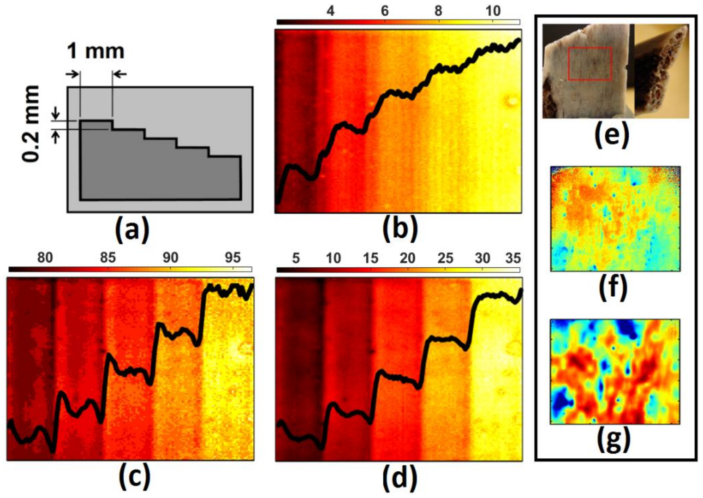
Figure 9a schematically shows the cross-section of a black plastic step wedge sample, simulating absorbers at different depths in a turbid medium. Figure 9b shows the conventional lock-in thermography phase image obtained at 3 Hz along with its mean profile over the steps. It can be seen that, although LI imaging can detect all the steps, it loses its depth resolution over deeper steps due to the diffuse nature of thermal waves. On the other hand, TCT imaging at the same modulation frequency and experimental conditions (averaging, laser power, etc.) maintains excellent resolution down to the deepest step in both peak delay time and phase images, Figure 9c,d respectively. This experiment clearly demonstrates that, compared to lock-in thermography, matched-filter thermography yields a more localized response in a diffusive field and improves the axial resolution while probing deep into the sample.
Figure 9e depicts the optical image of the interrogated surface of a goat bone along with its cross section. The optical image shows that the spongy trabecular bone is covered by the more dense cortical bone on the surface. Figure 9f shows the TCT phase image obtained at 10 Hz. Due to the relatively short thermal diffusion length at this frequency, the phase image reveals the structure of the cortical bone. However, reducing the excitation frequency to 1 Hz, and due to the depth selective nature of matched-filter thermography, the underlying trabecular structure can clearly be revealed (Figure 9g).
4.3. LIT vs. TWR vs. TCT
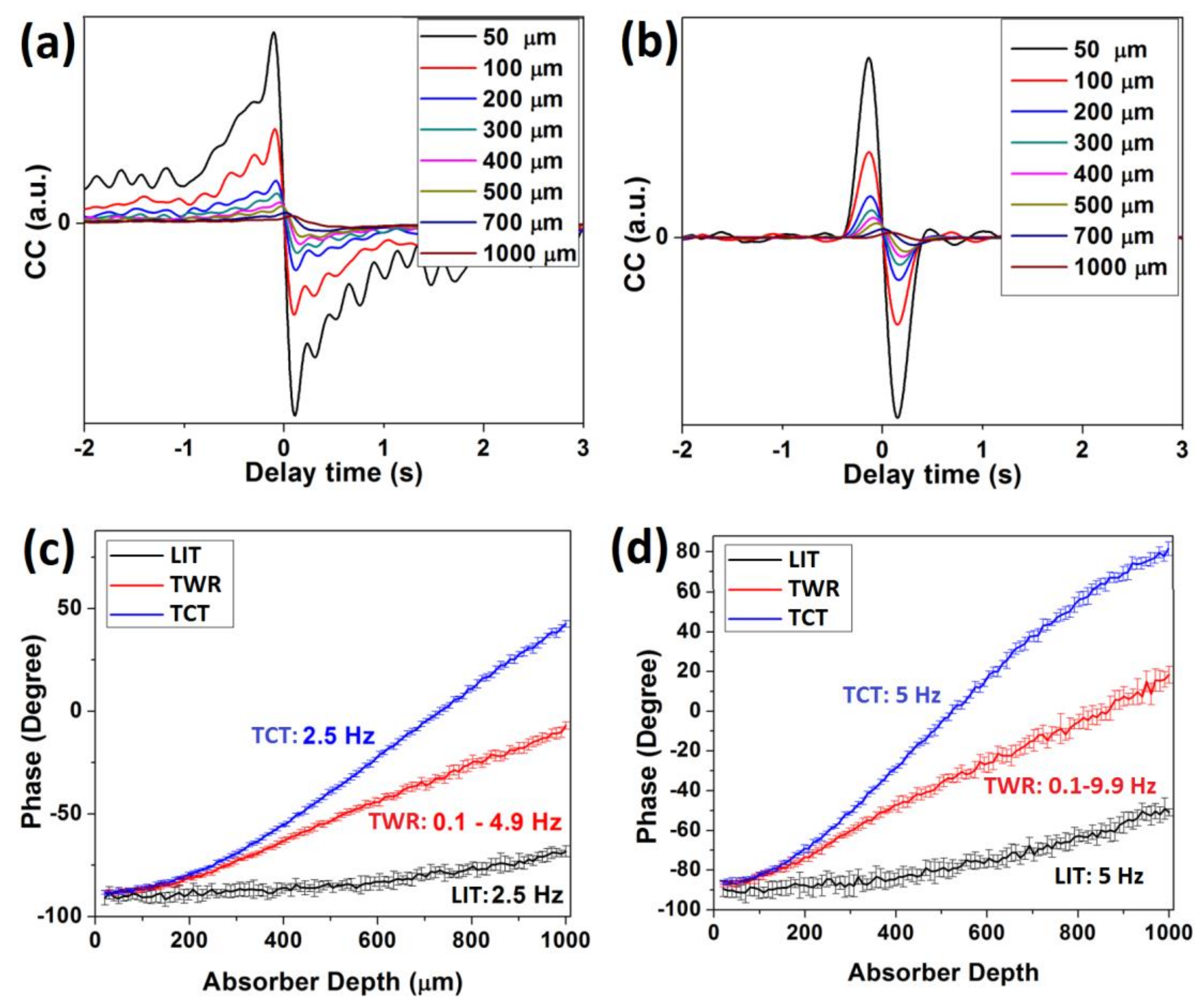
Although linear frequency modulation (chirp) and binary phase coding are both pulse compression techniques used for improving the axial/depth resolution of the matched filter, their implementation in thermal-wave fields yields different characteristics. Figure 10a plots the simulated responses of absorbers at various depths inside a turbid medium using TWR (0.1 Hz–4.9 Hz, 6.4 s). The TCT responses of the same simulated sample to an excitation at 2.5 Hz carrier frequency (i.e., the center frequency of TWR simulation) are depicted in Figure 10b. Comparison of these figures clearly shows that the narrow band nature of TCT results in more localized responses with minimal side lobes. These simulations suggest that, under similar experimental conditions, TCT is expected to outperform TWR in terms of depth resolution and SNR.
Figure 10c,d lie at the heart of this review paper in which the simulated performances of LIT, TWR, and TCT are compared. The spectra of the simulated responses were superposed with white noise (SNR = 1) to obtain more realistic results and simulations were repeated 10 times at each absorber depth for measurement of error bars. All other simulation conditions were kept the same. Figure 10c,d clearly shows the improvement of axial/depth resolution (the slope of the lines) when changing the modulation scheme from single frequency to LFM and finally to BPC modulation. Moreover, due to the higher SNR of matched filtering, the size of the error bars are smaller in TWR and TCT compared to that of the LIT.
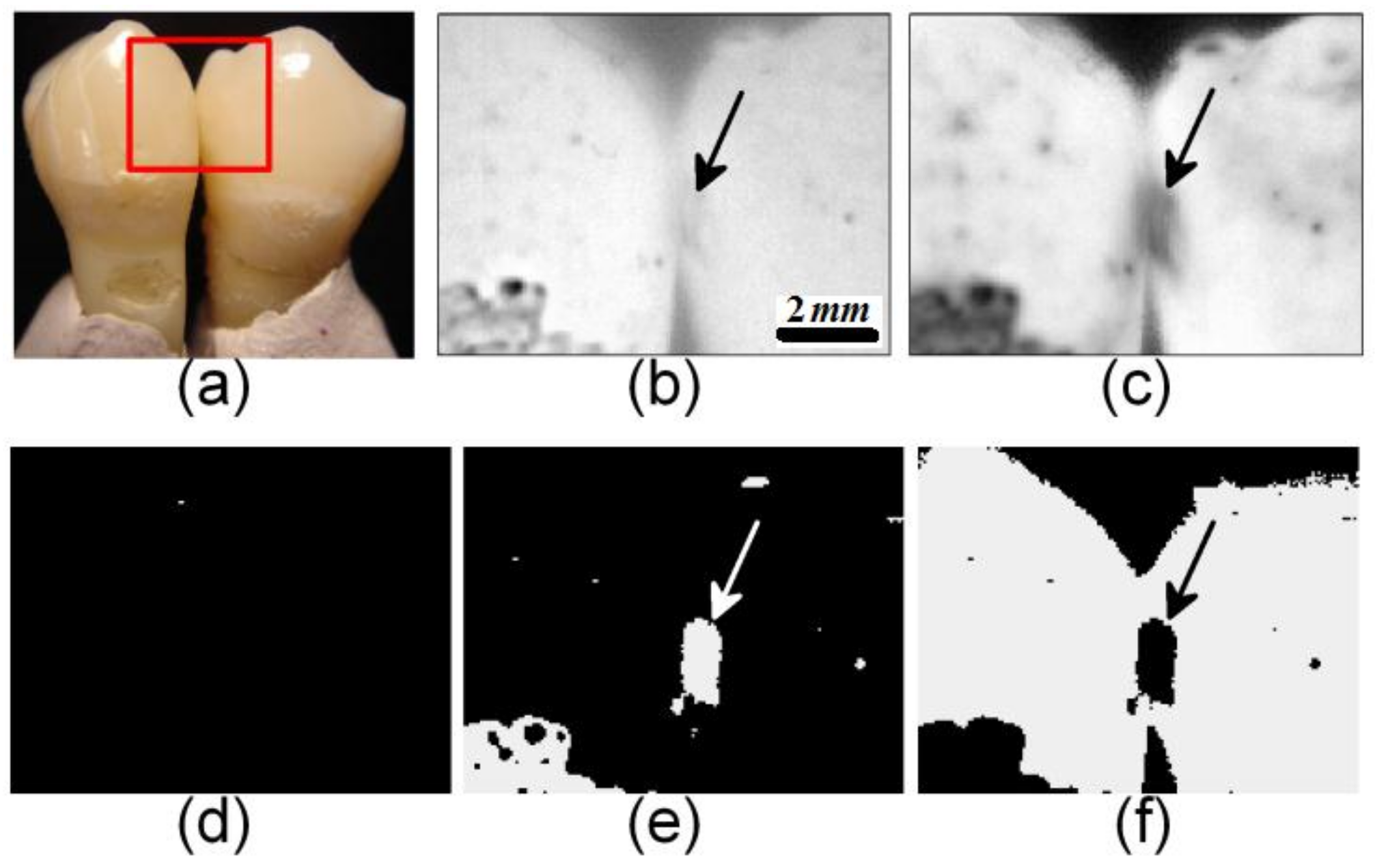
Figure 11 shows experimental results obtained from a teeth matrix. The contacting surface of the teeth has been demineralized (thus absorbs light) to simulate the challenging clinical scenario of interproximal early caries in the field of Dentistry. Comparison of LIT and TCT phase images, panels (b) and (c), formed under identical experimental conditions, clearly demonstrates the enhanced axial resolution of the TCT over LIT. Quantitative analysis of these images suggests a 275% increase in contrast between interproximal caries and the surrounding intact areas in TCT over that of LIT. Moreover, the enhancement of depth resolution in TCT allows one to construct iso-delay images in which thermal contributions from over and under layers are effectively suppressed. Figure 11d–f show thermal coherence tomographic images obtained through mathematical delaying of the filter by 2.7 ms, 29.7 ms, and 45.9 ms, respectively, and registering signals coherent to such delayed filters. No heat source can be observed in the first (i.e., shallowest) slice, while the deepest slice shows healthy enamel areas. Defects and caries shift the thermal-wave centroid closer to the interrogated surface (compared to the surrounding healthy enamel) and, as a result, are revealed in the intermediate slice (Figure 11e).
The results of Figure 11, experimentally, demonstrate that, by improving the axial resolution, TCT allows for deconvolution of thermal responses of subsurface defects from those of the non-defective regions.
5. Future Directions
To date, most of the research in the field of matched-filter thermography has been focused on exploring the advantages of the matched-filter approach over conventional thermography techniques through theoretical modeling and experimentation on standardized samples. Optimization of excitation and signal detection parameters have also been explored. Future directions desired in the field include: standardization of methodologies developed so far through consensus reports or development of standard procedures by regulating bodies such ISO or ASTM; development of strategies and methodologies for quantification of defect and/or material properties from matched-filter responses; and development of strategies for lowering the cost of thermography systems to enable translation/commercialization to industry and medicine.
6. Summary
This paper reviews the basic principles and experimental results of matched-filter thermography such as the thermal-wave responses to matched-filter thermography using two major pulse compression techniques (i.e., linear frequency modulation and binary phase coding) from both theoretical and experimental perspectives. Both simulations and experimental works reported to date suggest that incorporation of matched-filtering in thermography allows one to maintain good axial resolution while inspecting deep into opaque and turbid media, overcoming the classic limitation of conventional pulsed and lock-in thermography. Moreover, recent works in the field suggest that scanning the matched-filter allows one to create iso-delay images, and thus enables deconvolution of thermal responses of defective regions from those of the non-defective regions.
Acknowledgments
N.T. is grateful to the Natural Sciences and Engineering Research Council of Canada for the award of a Discovery Grant (RGPIN-2015-03666), to the Canadian Institutes of Health Research for the award of a Collaborative Health Research Projects Grant (DAN381313), and to the Lassonde School of Engineering and the York University for their financial support.
Conflicts of Interest
The author declares no conflict of interest. The funding sponsors had no role in the design of the study; in the collection, analyses, or interpretation of data; in the writing of the manuscript, and in the decision to publish the results.
References
- Milne, J.M.; Reynolds, W.N. The Non-Destructive Evaluation of Composites and Other Materials by Thermal Pulse Video Thermography; SPIE; Cambridge Symposium: Cambridge, UK, 1984; p. 4. [Google Scholar]
- Cheng, L.; Tian, G.Y. Surface Crack Detection for Carbon Fiber Reinforced Plastic (CFRP) Materials Using Pulsed Eddy Current Thermography. IEEE Sens. J. 2011, 11, 3261–3268. [Google Scholar] [CrossRef]
- Wu, D.; Salerno, A.; Malter, U.; Aoki, R.; Kochendörfer, R.; Kächele, P.; Woithe, K.; Pfister, K.; Busse, G. Inspection of aircraft structural components using lockin-thermography. Quant. Infrared Thermogr. QIRT 1996, 96, 251–256. [Google Scholar]
- Breitenstein, O.; Langenkamp, M.; Altmann, F.; Katzer, D.; Lindner, A.; Eggers, H. Microscopic lock-in thermography investigation of leakage sites in integrated circuits. Rev. Sci. Instrum. 2000, 71, 4155–4160. [Google Scholar] [CrossRef]
- Telenko, S.A.; Vargas, G.; Nelson, J.S.; Milner, T.E. Coherent thermal wave imaging of subsurface chromophores in biological materials. Phys. Med. Biol. 2002, 47, 657–671. [Google Scholar] [CrossRef] [PubMed]
- Lee, P.; Ho, K.K.Y.; Lee, P.; Greenfield, J.R.; Ho, K.K.Y.; Greenfield, J.R. Hot fat in a cool man: Infrared thermography and brown adipose tissue. Diabetes Obes. Metab. 2011, 13, 92–93. [Google Scholar] [CrossRef] [PubMed]
- Tabatabaei, N.; Mandelis, A.; Amaechi, B.T. Thermophotonic lock-in imaging of early demineralized and carious lesions in human teeth. J. Biomed. Opt. 2011, 16, 071402. [Google Scholar] [CrossRef] [PubMed]
- Tabatabaei, N.; Mandelis, A.; Dehghany, M.; Michaelian, K.H.; Amaechi, B.T. On the sensitivity of thermophotonic lock-in imaging and polarized Raman spectroscopy to early dental caries diagnosis. J. Biomed. Opt. 2012, 17, 025002. [Google Scholar] [CrossRef] [PubMed]
- Ojaghi, A.; Parkhimchyk, A.; Tabatabaei, N. First step toward translation of thermophotonic lock-in imaging to dentistry as an early caries detection technology. J. Biomed. Opt. 2016, 21, 96003. [Google Scholar] [CrossRef] [PubMed]
- Razani, M.; Parkhimchyk, A.; Tabatabaei, N. Lock-in thermography using a cellphone attachment infrared camera. AIP Adv. 2018, 8, 035305. [Google Scholar] [CrossRef]
- Ojaghi, A.; Parkhimchyk, A.; Tabatabaei, N. Long-Wave Infrared Thermophotonic Imaging of Demineralization in Dental Hard Tissue. Int. J. Thermophys. 2016, 37, 85. [Google Scholar]
- Ojaghi, A.; Pallapa, M.; Tabatabaei, N.; Rezai, P. High-sensitivity interpretation of lateral flow immunoassays using thermophotonic lock-in imaging. Sens. Actuators A Phys. 2018, 273, 189–196. [Google Scholar] [CrossRef]
- Ko, A.C.-T.; Choo-Smith, L.-P.I.; Hewko, M.D.; Leonardi, L.; Sowa, M.G.; Dong, C.C.C.S.; Williams, P.; Cleghorn, B. Ex vivo detection and characterization of early dental caries by optical coherence tomography and Raman spectroscopy. J. Biomed. Opt. 2005, 10, 16. [Google Scholar] [CrossRef] [PubMed]
- Amaechi, B.T.; Higham, S.M.; Podoleanu, A.G.; Rogers, J.A.; Jackson, D.A. Use of optical coherence tomography for assessment of dental caries: Quantitative procedure. J. Oral Rehabilit. 2001, 28, 1092–1093. [Google Scholar] [CrossRef]
- Wijesinghe, R.; Cho, N.; Park, K.; Jeon, M.; Kim, J. Bio-Photonic Detection and Quantitative Evaluation Method for the Progression of Dental Caries Using Optical Frequency-Domain Imaging Method. Sensors 2016, 16, 2076. [Google Scholar] [CrossRef] [PubMed]
- Breitenstein, O.; Warta, W.; Langenkamp, M. Lock-In Thermography; Springer: Berlin, Germany, 2003. [Google Scholar]
- Jäckel, P.; Netzelmann, U. The influence of external magnetic fields on crack contrast in magnetic steel detected by induction thermography. Quant. InfraRed Thermogr. J. 2013, 10, 237–247. [Google Scholar] [CrossRef]
- Krstulovic-Opara, L.; Klarin, B.; Neves, P.; Domazet, Z. Thermal imaging and Thermoelastic Stress Analysis of impact damage of composite materials. Eng. Fail. Anal. 2011, 18, 713–719. [Google Scholar] [CrossRef]
- Mendioroz, A.; Celorrio, R.; Salazar, A. Ultrasound excited thermography: An efficient tool for the characterization of vertical cracks. Meas. Sci. Technol. 2017, 28, 112001. [Google Scholar] [CrossRef]
- Wu, D.; Salerno, A.; Malter, U.; Aoki, R.; Woithe, K.; Pfister, K.; Busse, G. Inspection of Aircraft Structural Components Using Lockin-Thermography; AIPnD: Brescia, Italy, 1997. [Google Scholar]
- Tabatabaei, N.; Mandelis, A. Thermal-wave radar: A novel subsurface imaging modality with extended depth-resolution dynamic range. Rev. Sci. Instrum. 2009, 80, 034902. [Google Scholar] [CrossRef] [PubMed]
- Tabatabaei, N.; Mandelis, A. Thermal Coherence Tomography Using Match Filter Binary Phase Coded Diffusion Waves. Phys. Rev. Lett. 2011, 107, 165901. [Google Scholar] [CrossRef] [PubMed]
- Tabatabaei, N.; Mandelis, A.; Amaechi, B.T. Thermophotonic radar imaging: An emissivity-normalized modality with advantages over phase lock-in thermography. Appl. Phys. Lett. 2011, 98, 163706. [Google Scholar] [CrossRef]
- Mulaveesala, R.; Tuli, S. Theory of frequency modulated thermal wave imaging for nondestructive subsurface defect detection. Appl. Phys. Lett. 2006, 89, 191913. [Google Scholar] [CrossRef]
- Mulaveesala, R.; Vaddi, J.S.; Singh, P. Pulse compression approach to infrared nondestructive characterization. Rev. Sci. Instrum. 2008, 79, 094901. [Google Scholar] [CrossRef] [PubMed]
- Tabatabaei, N.; Mandelis, A. Thermal Coherence Tomography: Depth-Resolved Imaging in Parabolic Diffusion-Wave Fields Using the Thermal-Wave Radar. Int. J. Thermophys. 2012, 33, 1989–1995. [Google Scholar] [CrossRef]
- Turin, G. An introduction to matched filters. IRE Trans. Inf. Theory 1960, 6, 311–329. [Google Scholar] [CrossRef]
- Vleck, J.H.V.; Middleton, D. A Theoretical Comparison of the Visual, Aural, and Meter Reception of Pulsed Signals in the Presence of Noise. J. Appl. Phys. 1946, 17, 940–971. [Google Scholar] [CrossRef]
- Kirkbright, G.F.; Miller, R.M. Cross-correlation techniques for signal recovery in thermal wave imaging. Anal. Chem. 1983, 55, 502–506. [Google Scholar] [CrossRef]
- Mandelis, A. Frequency modulated (FM) time delay photoacoustic and photothermal wave spectroscopies. Technique, instrumentation, and detection. Part I: Theoretical. Rev. Sci. Instrum. 1986, 57, 617–621. [Google Scholar] [CrossRef]
- Mandelis, A.; Borm, L.M.L.; Tiessinga, J. Frequency modulated (FM) time delay photoacoustic and photothermal wave spectroscopies. Technique, instrumentation, and detection. Part II: Mirage effect spectrometer design and performance. Rev. Sci. Instrum. 1986, 57, 622–629. [Google Scholar] [CrossRef]
- Mandelis, A.; Borm, L.L.M.; Tiessinga, J. Frequency modulated (FM) time delay photoacoustic and photothermal wave spectroscopies. Technique, instrumentation, and detection. Part III: Mirage effect spectrometer, dynamic range, and comparison to pseudo-random-binary-sequence (PRBS) method. Rev. Sci. Instrum. 1986, 57, 630–635. [Google Scholar] [CrossRef]
- Liu, J.; Gong, J.; Qin, L.; Wang, H.; Wang, Y. Study of inspection on metal sheet with subsurface defects using linear frequency modulated ultrasound excitation thermal-wave imaging (LFM-UTWI). Infrared Phys. Technol. 2014, 62, 136–142. [Google Scholar] [CrossRef]
- Wang, F.; Liu, J.; Liu, Y.; Wang, Y. Research on the fiber lay-up orientation detection of unidirectional CFRP laminates composite using thermal-wave radar imaging. NDT E Int. 2016, 84, 54–66. [Google Scholar] [CrossRef]
- Velazquez-Hernandez, R.; Melnikov, A.; Mandelis, A.; Sivagurunathan, K.; Rodriguez-Garcia, M.E.; Garcia, J. Non-destructive measurements of large case depths in hardened steels using the thermal-wave radar. NDT E Int. 2012, 45, 16–21. [Google Scholar] [CrossRef]
- Wang, F.; Liu, J.; Liu, Y.; Wang, Y.; Gong, J. Detection of Fiber Layer-Up Lamination Order of CFRP Composite Using Thermal-Wave Radar Imaging. Int. J. Thermophys. 2016, 37, 97. [Google Scholar] [CrossRef]
- Gong, J.; Liu, J.; Qin, L.; Wang, Y. Investigation of carbon fiber reinforced polymer (CFRP) sheet with subsurface defects inspection using thermal-wave radar imaging (TWRI) based on the multi-transform technique. NDT E Int. 2014, 62, 130–136. [Google Scholar] [CrossRef]
- Yang, R.; He, Y. Pulsed inductive thermal wave radar (PI-TWR) using cross correlation matched filtering in eddy current thermography. Infrared Phys. Technol. 2015, 71, 469–474. [Google Scholar] [CrossRef]
- Busse, G.; Wu, D.; Karpen, W. Thermal wave imaging with phase sensitive modulated thermography. J. Appl. Phys. 1992, 71, 3962–3965. [Google Scholar] [CrossRef]
- Kaiplavil, S.; Mandelis, A. Highly depth-resolved chirped pulse photothermal radar for bone diagnostics. Rev. Sci. Instrum. 2011, 82, 29. [Google Scholar] [CrossRef] [PubMed]
- Kaiplavil, S.; Mandelis, A. Truncated-correlation photothermal coherence tomography for deep subsurface analysis. Nat. Photonics 2014, 8, 635–642. [Google Scholar] [CrossRef]
- Kaiplavil, S.; Mandelis, A.; Wang, X.; Feng, T. Photothermal tomography for the functional and structural evaluation, and early mineral loss monitoring in bones. Biomed. Opt. Express 2014, 5, 2488–2502. [Google Scholar] [CrossRef] [PubMed]
- Kaiplavil, S.; Mandelis, A.; Amaechi, B.T. Truncated-correlation photothermal coherence tomography of artificially demineralized animal bones: Two- and three-dimensional markers for mineral loss monitoring. J. Biomed. Opt. 2014, 19, 026015. [Google Scholar] [CrossRef] [PubMed]
- Tavakolian, P.; Sivagurunathan, K.; Mandelis, A. Enhanced truncated-correlation photothermal coherence tomography with application to deep subsurface defect imaging and 3-dimensional reconstructions. J. Appl. Phys. 2017, 122, 1239–1247. [Google Scholar] [CrossRef]
- Dua, G.; Mulaveesala, R. Applications of barker coded infrared imaging method for characterisation of glass fibre reinforced plastic materials. Electron. Lett. 2013, 49, 1071–1073. [Google Scholar] [CrossRef]
- Mulaveesala, R.; Arora, V. Complementary coded thermal wave imaging scheme for thermal non-destructive testing and evaluation. Quant. InfraRed Thermogr. J. 2017, 14, 44–53. [Google Scholar] [CrossRef]
- Arora, V.; Mulaveesala, R. Application of golay complementary coded excitation schemes for non-destructive testing of sandwich structures. Opt. Lasers Eng. 2017, 93, 36–39. [Google Scholar] [CrossRef]
- Geetika, D.; Ravibabu, M.; Juned, A.S. Effect of spectral shaping on defect detection in frequency modulated thermal wave imaging. J. Opt. 2015, 17, 025604. [Google Scholar]
- Mandelis, A. Diffusion-Wave Fields: Mathematical Methods and Green Functions; Springer: New York, NY, USA, 2013. [Google Scholar]
- Rohling, H.; Plagge, W. Mismatched-filter design for periodic binary phased signals. IEEE Trans. Aerosp. Electron. Syst. 1989, 25, 890–897. [Google Scholar] [CrossRef]
Figure 1.
Simulated filter, noisy response, and matched-filter output for: (a–c) single-frequency response of a single reflector; (d–f) single-frequency response of two reflectors; (g–i) Linear frequency modulation (LFM) response of single reflector; LFM response of two reflectors.
Figure 1.
Simulated filter, noisy response, and matched-filter output for: (a–c) single-frequency response of a single reflector; (d–f) single-frequency response of two reflectors; (g–i) Linear frequency modulation (LFM) response of single reflector; LFM response of two reflectors.

Figure 2.
Schematic models of (a) an opaque sample with blind holes of various depths and (b) a turbid sample with absorber at various depths [21].
Figure 2.
Schematic models of (a) an opaque sample with blind holes of various depths and (b) a turbid sample with absorber at various depths [21].

Figure 3.
Simulated (a) spectral responses and (b) Thermal-wave radar (TWR) subtractive surface temperature evolution over blind holes of different thicknesses; (c) simulated TWR outputs for 100 µm thick and semi-infinite steel samples; (d) variation of TWR peak delay time with opaque sample thickness in normal and subtraction modes; (e) effect of TWR excitation waveform parameters on detectability of defects; (f) variation of TWR peak delay time with absorber depth in turbid medium [21].

Figure 4.
Schematic presentation of TWR experimental setups using (a) a single detector [23] and (b) an infrared camera [23], (c) signal processing block diagram of TWR [23].
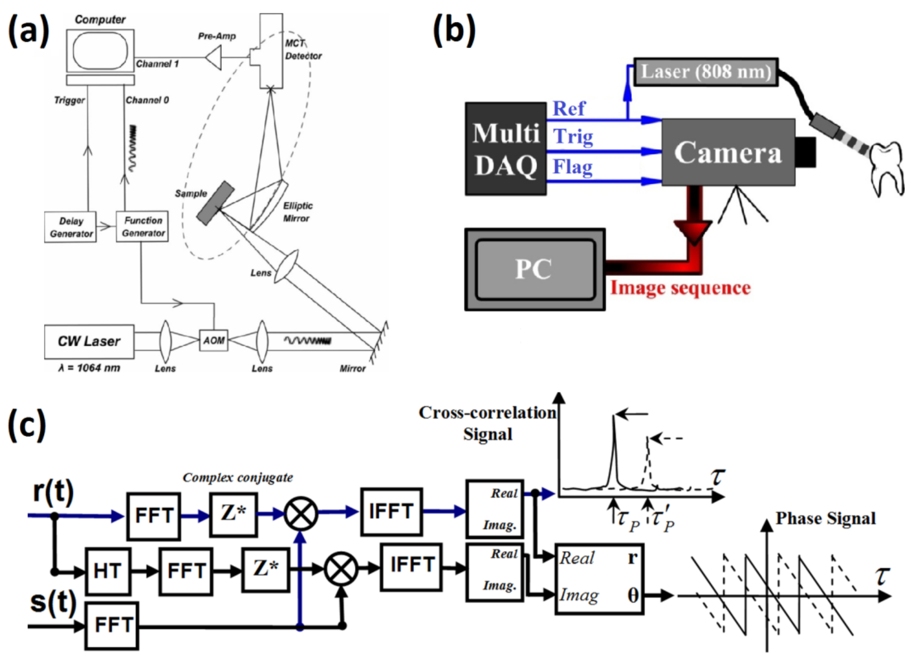
Figure 5.
Experimental results obtained using (a,b) single-frequency photothermal radiometry and (c,d) TWR in an opaque sample with blind holes. Remaining thickness of holes are depicted in the insert; (e) experimental TWR responses from glass slides of various thicknesses painted on the black on the front or back surface [21].
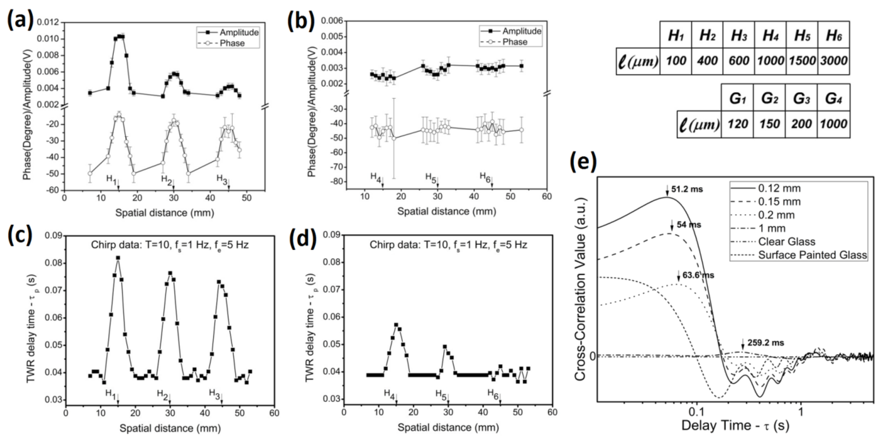
Figure 6.
TWR imaging of transparent sample with iso-depth absorbers of different absorption coefficients using (a) Cross-correlation (CC) amplitude (unit: a.u.); (b) CC peak delay time (unit: millisecond); (c) CC phase (unit: degree) and their mean horizontal profiles; (d–f), respectively. Chirp parameters: 0.01–1 Hz in 6 s.
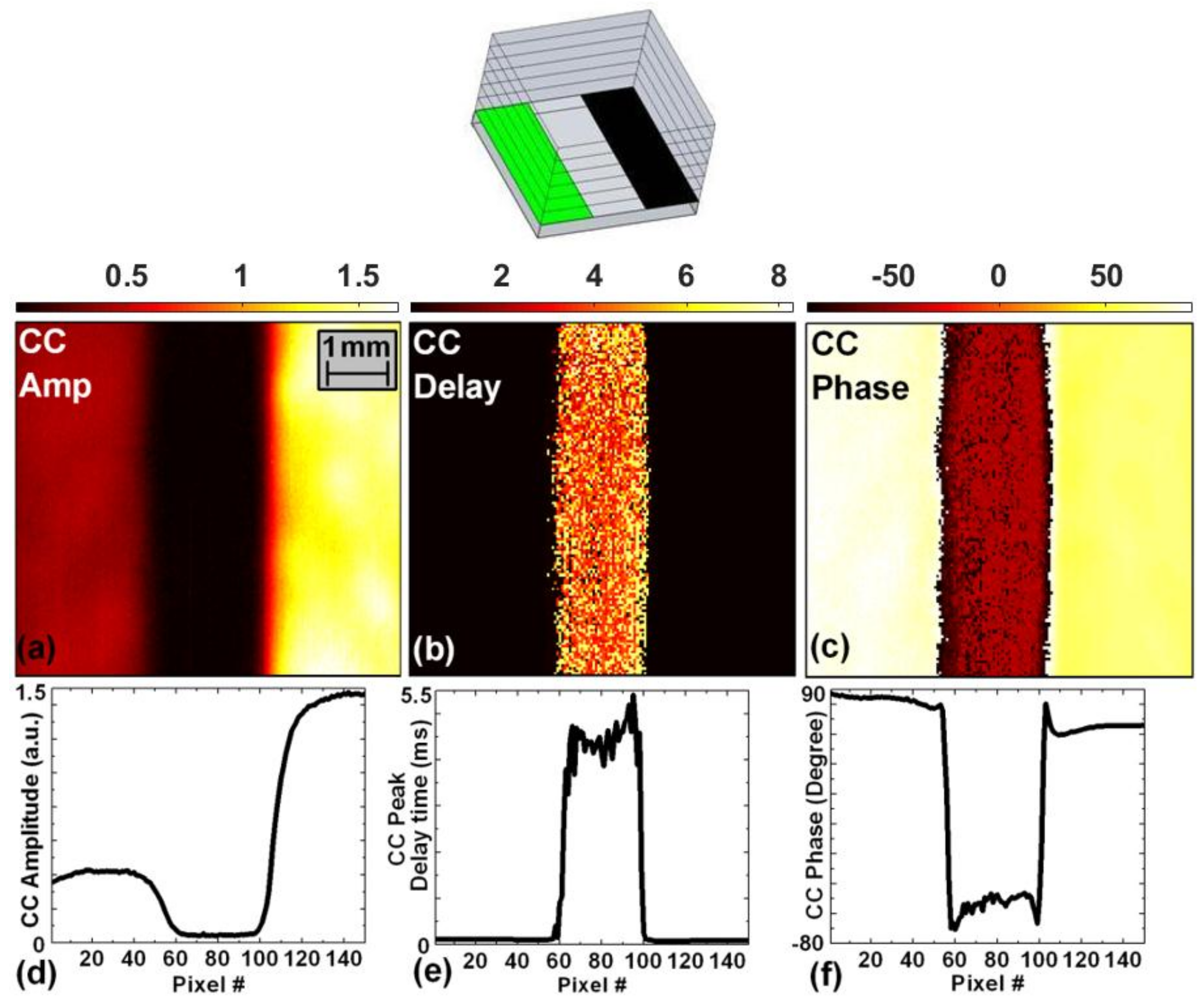
Figure 7.
Schematic procedure of Binary Phase Coding (BPC) signal construction in time (top) and frequency (bottom) domains for a 7-bit code and 5 Hz carrier [22].
Figure 7.
Schematic procedure of Binary Phase Coding (BPC) signal construction in time (top) and frequency (bottom) domains for a 7-bit code and 5 Hz carrier [22].

Figure 8.
Theoretical CC (a) phase; (b) peak delay time (left and bottom axis) and amplitude (right and top axis) curves as a function of the subsurface absorber depth using properties of dental enamel: μa = 100 [m−1], μs = 6000 [m−1], g = 0.96, r = 0.65, k = 0.9 [Wm−1k−1], α = 5 × 10⁻⁷ [m2s−1]. The numbers accompanying the curves determine the carrier frequency according to the inset of part (a) [22].

Figure 9.
(a) cross section of step wedge light-absorbing inclusion in a turbid medium; (b) conventional lock-in thermography (LIT) phase (unit: degree); (c) BPC peak delay time (unit: millisecond); and (d) BPC phase images (unit: degree) of the step wedge sample using thermal coherence tomography (TCT) (16-bit code). The curve in each image shows the mean horizontal profile of the corresponding contrast parameter; (e) pictures of the interrogated surface and cross section of a goat bone; TCT phase images of goat bone at (f) 10 Hz and (g) 1 Hz carrier frequencies [22].

Figure 10.
Simulated (a) TWR (0.1 Hz–4.9 Hz, 6.4 s) and (b) TCT (2.5 Hz, 16-bit coding) responses of turbid sample containing absorbers at several depths. Comparison of simulated phase responses using LIT, TWR, and TCT for absorbers in turbid medium. Turbid medium properties: μa = 100 [m−1], μs = 6000 [m−1], g = 0.96, r = 0.65, k = 0.9 [Wm−1k−1], α = 5 × 10⁻⁷ [m2s−1].

Figure 11.
(a) teeth matrix with hidden inter-proximal early caries. The rectangle shows the imaged area; (b) conventional LIT and (c) BPC phase images; TCT images obtained at (d) 2.7ms; (e) 29.7 ms; and (f) 45.9 ms delay times. The white color depicts the pixels coherent to the delayed matched filter. The arrow indicates the hidden interproximal caries [22].
© 2018 by the authors. Licensee MDPI, Basel, Switzerland. This article is an open access article distributed under the terms and conditions of the Creative Commons Attribution (CC BY) license (http://creativecommons.org/licenses/by/4.0/).
Share and Cite
MDPI and ACS Style
Tabatabaei, N. Matched-Filter Thermography. Appl. Sci. 2018, 8, 581. https://doi.org/10.3390/app8040581
AMA Style
Tabatabaei N. Matched-Filter Thermography. Applied Sciences. 2018; 8(4):581. https://doi.org/10.3390/app8040581
Chicago/Turabian StyleTabatabaei, Nima. 2018. "Matched-Filter Thermography" Applied Sciences 8, no. 4: 581. https://doi.org/10.3390/app8040581
Note that from the first issue of 2016, this journal uses article numbers instead of page numbers. See further details here.