Optimal Piezoelectric Potential Distribution for Controlling Multimode Vibrations


Dipartimento di Ingegneria, Università degli Studi Roma Tre, Via della Vasca Navale, 79, 00146 Roma, Italy
*
Author to whom correspondence should be addressed.
Appl. Sci. 2018, 8(4), 551; https://doi.org/10.3390/app8040551
Submission received: 15 March 2018
/
Revised: 29 March 2018
/
Accepted: 30 March 2018
/
Published: 3 April 2018
(This article belongs to the Section Mechanical Engineering)
Abstract
:Vibration damping is prominent in engineering; in fact, vibrations are related to many phenomena (e.g., the fatigue of structural elements). The advent of smart materials has significantly increased the number of available solutions in this field. Among smart materials, piezoelectric materials are most promising. However, their efficiency depends on their placement. There are many studies on their optimal placement for damping a particular mode, but few account for multimodal vibrations damping. In a previous work, an analytical method was proposed to find the optimal placement of piezoelectric plates to control the multimode vibrations of a cantilever beam. In this study, the efficiency of the above method has been improved, considering all plates active simultaneously, regardless of the eigenmodes that are excited, and changing, instead of the plates, the potential distribution. The method results indicate the optimal potential distribution for different excited eigenmodes. The results have been compared with those obtained by experimental tests and numerical simulations, exhibiting very good agreement.
1. Introduction
Vibrations in flexible and lightweight structures are often a matter of concern for mechanical and aeronautical engineers since they promote the formation of cracks that weaken the mechanical components and lower their fatigue resistance. In order to increase their efficiency, the aerospace and mechanical industries have made extensive use of lightweight, robust, and low-cost materials. In gas turbine engines, for example, the vibrations result from the interaction between the fluid and the blades, and vibration reduction systems are widely used to increase the fatigue life of mechanical components [1,2,3,4]. Damping systems can be classified into passive and active: The former exhibit good effectiveness, low complexity, and low cost, but show a small bandwidth. The latter present a large bandwidth and can adapt their features to time-dependent loads, so these are more efficient than a passive system. Smart materials developed in the last several decades have shown a great potential for monitoring and control applications and, among these piezoelectric materials, are the most frequently used when a high frequency and a high transient response is required [5,6]. These materials are unique because their mechanical behavior is related to their electric behavior and vice versa [7]. In particular, the strains induce an electric field (a direct effect) and vice versa (an inverse effect). This peculiarity enhanced its applicability in many engineering sectors. One of the materials most commonly used in vibration control applications is lead zirconate titanate (PZT) [8,9]. However, the efficiency of the PZT plates, to damp single-mode or multimode vibrations, depends strictly on their placement. PZT element optimal placement usually concerns the minimization or maximization of an objective function [10,11]. Early studies on single-mode attenuation were carried out by [7]. The evidence reveals that the element should be placed in the highest average deformation area, and further studies seem to support this result [12,13]. If a cantilever beam is considered, the maximum damping effect occurs when the element is placed close to the joint [14,15,16]. In the simply supported beam case, it has been demonstrated by [17] that the maximum attenuation of a single mode occurs if the PZT lies in the region between the nodal lines. The studies of Barboni et al. [18] show that, in order to excite a specific single flexural mode of an Euler–Bernoulli beam, the actuator must be placed within two consecutive zero curvature points. Further studies have been performed to identify the optimal size and positioning of two pairs of PZT plates, in the case of different constraint conditions [19]. Other researchers analyzed the interaction between damping efficacy and the material and bonding layer thicknesses [20], and the outcomes suggest that the actuators have to be placed in an extensive strain zone. Single-mode and multimodal vibrations were examined by [21]. Their work focused on two pairs of piezoelectric actuators placed on a beam, and a new index of control has been proposed.
In this paper, the concept of the optimal placement is traced back to the concept of the optimal potential distribution, which is the potential distribution on all the piezoelectric plates that cover all the beam, where maximum damping is achieved. In this way, a more efficient system is obtained. In fact, in this manner, the piezoelectric plates will always work to damp the vibrations (in every condition and combination of modes) and have the potential that changes its distribution so that they can always work in optimal conditions. In a previous paper [22], one of the authors proposed a new method to damp the multimodal vibrations. In this work, a further new model is developed and verified by experimental tests and numerical simulations. The results show that there is good agreement between those of the model and those of the experimental tests and numerical simulations.
2. Governing Equations for a Piezoelectric Coupled Beam
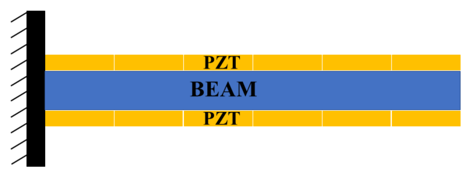
In Figure 1, a scheme of the piezoelectric coupled beam is reported.
Where , , and indicate the work of external, inertial, applied, and piezoelectric forces, respectively, the virtual work principle can be written as
The calculus of has been confirmed by many studies (one of the first studies in this regard was conducted by Crawley et al. ([7]) in 1987), and experimental evidence shows that, in the case of perfectly bonded material interfaces, the stresses that a plate applies to the beam are concentrated at the ends of the plate. Therefore, by applying two harmonic voltages opposite in the phase between the upper plate and the lower plate, such action can be modeled by a couple of flexural moments M concentrated at their ends (Figure 2).
If
the flexural moment can be written as ([7])
and will be
where represents the points where the potential changes its sign, so that will be or depending on the potential distribution on the plate i (Figure 2). The optimization problem can be traced back to the research of the optimal distribution of the or, in other words, to the research of the optimal distribution of the points .
By introducing the inertial, internal, and external forces in Equation (1) and applying the modal analysis technique, the following equilibrium equation is obtained
where M and K are, respectively, the mass and the stiffness matrix, X is the vector of the modal amplitudes, and the vector B is
where .
If the viscous damping is added, Equation (5) becomes:
Assuming that are the orthonormal modes, it follows that is the identity matrix and that is the natural frequencies matrix . If is related to the Rayleigh damping () where , Equation (7) can be written as
Since the flexural eigenmode of the cantilever beam achieves its maximum displacement amplitude at the free end, this point has been chosen as a reference point for the vibrations of the whole cantilever beam. Indicating with and the free end displacement due to, respectively, the load F and the piezoelectric load, the total displacement can be written as as a consequence of the linearity of the system. Choosing a suitable spectrum load, it is possible to activate the piezoelectric plate to obtain opposite in phase with respect to , so that, indicating with , and the amplitudes of the relative displacements, . In this paper, the optimal potential distribution has been considered as the one that minimizes the amplitude of so that the optimal distribution will be the one that, for the same V, maximizes . It can be demonstrated that ([22]), without taking into account the transient part,
where are the excited modes.
Choosing a load that excites two modes, indicating with and the excited modes and considering a parameter r that takes into account the distribution of the load between the two eigenfrequencies, the following can be written:
To achieve the maximum efficiency (or, as mentioned above, in order to obtain opposite in phase to ), the spectrum of the potential distribution has been chosen with the same characteristics of the load ([22]) and parameterized by the same parameter:
Substituting Equation (11) in Equation (9),
which can be written in the form
where has been chosen to cover the entire beam with the piezoelectric plates. In order to find the other points , it is helpful to introduce the following function:
This is obtained by a linear combination of two oscillating functions and presents an alternating maximum and minimum. It can be observed that the optimal potential distribution is obtained when the points coincide with the extrema of . In particular, considering that the function assumes its maximum positive value in ,
it is convenient to choose in Equation (13). Moreover, comparing with Equation (13), it can be noticed that, to obtain the maximum value of , must coincide with the first minimum of closer to , choosing , the point must coincide with the first maximum of closer to , choosing , etc. In this manner, will be
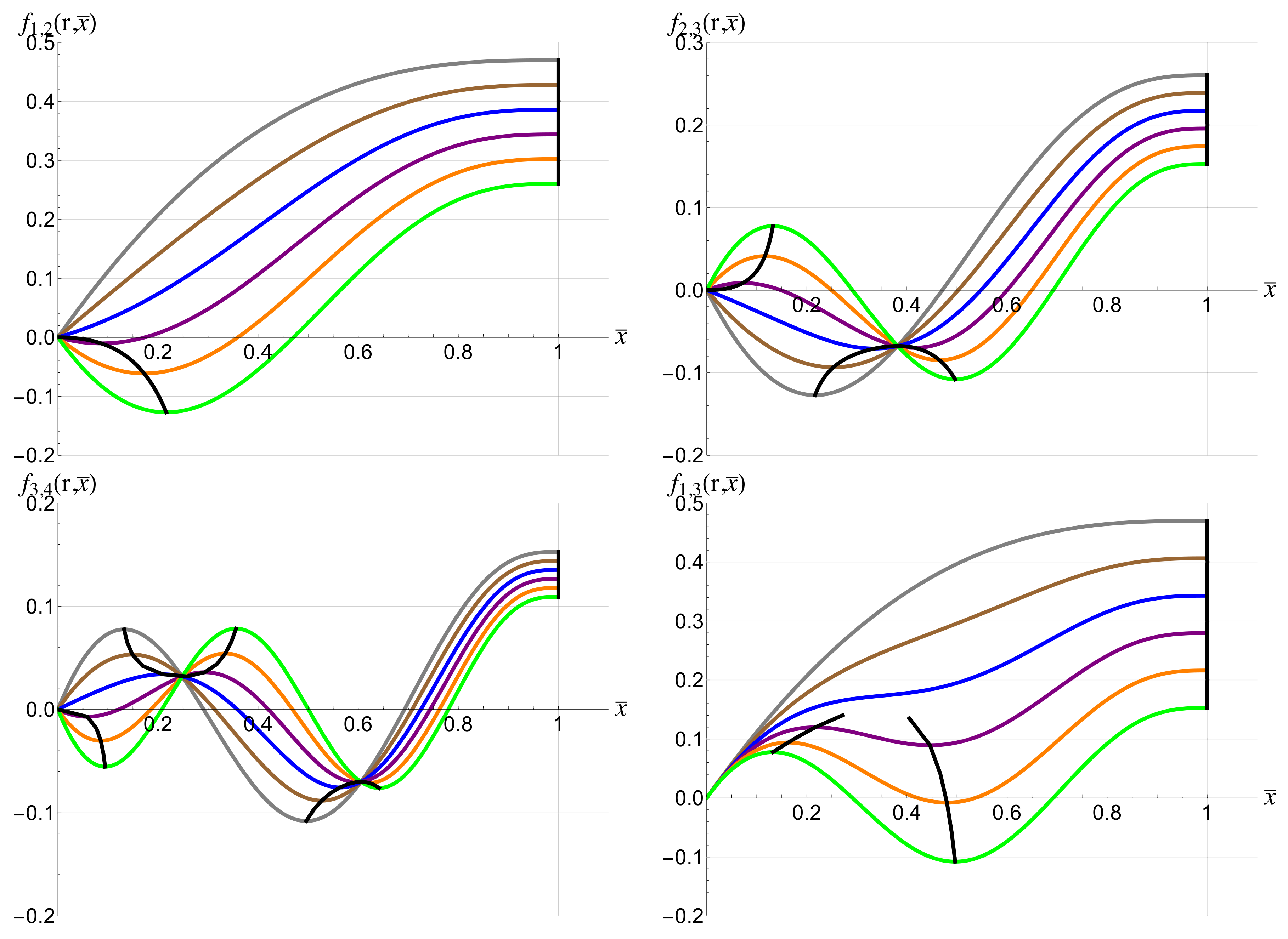
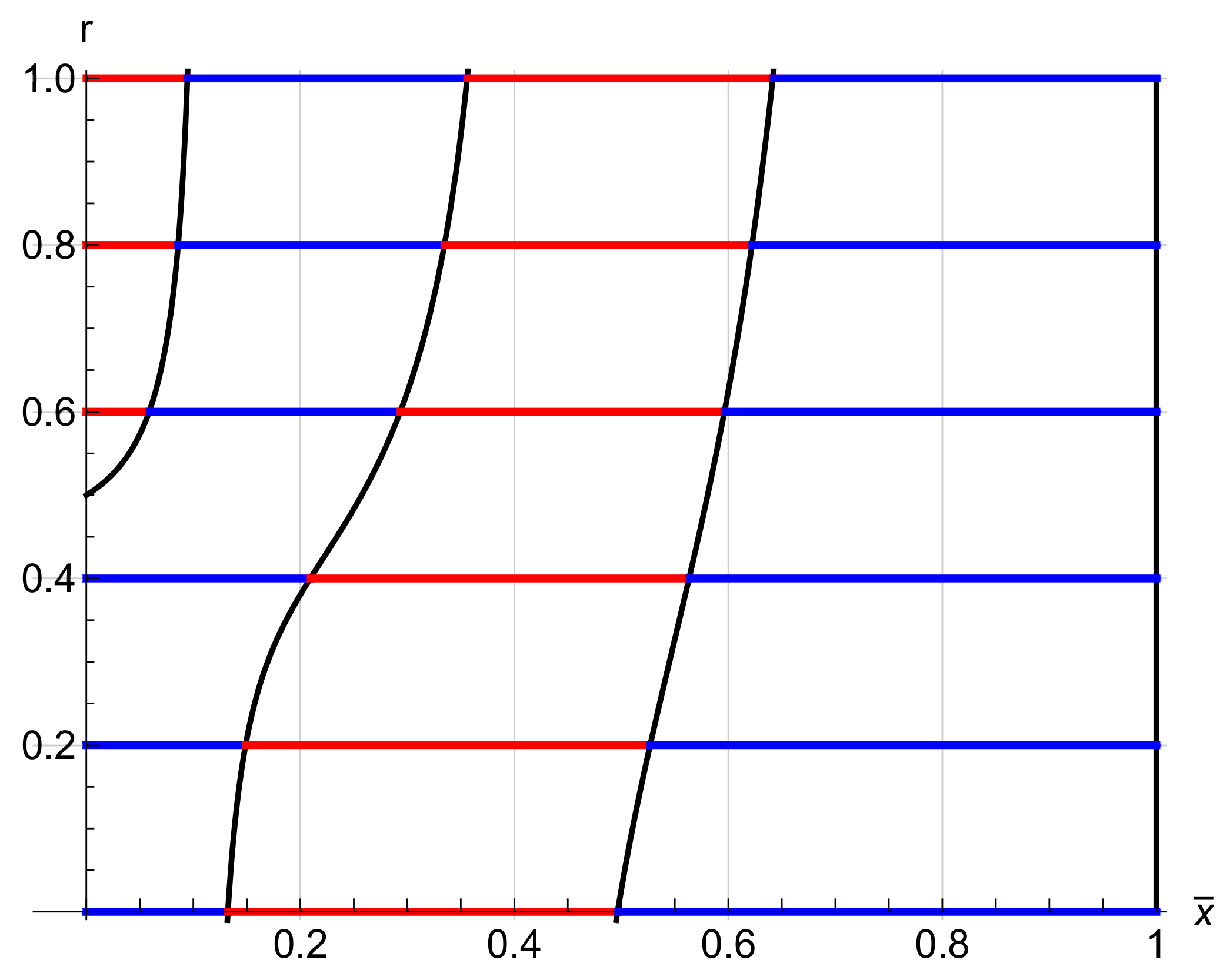
In Figure 3, the functions for different combinations of the first four eigenmodes, and various values of r, are reported. The black lines represent the “paths” of an extrema point when r changes, i.e., at the intersections between the black lines, and identifies the point where the potential must change its sign.
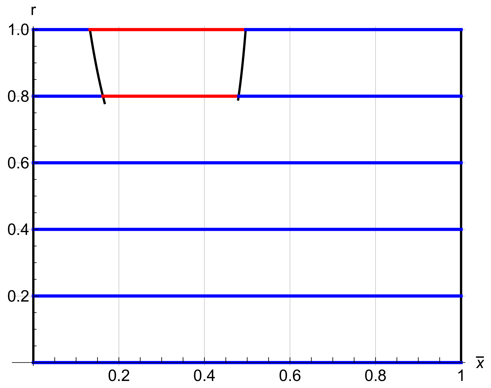
In what follows, for the sake of example, the coupling between the first two modes is considered, and the black curves in the plane are represented.
3. Experimental and Numerical Tests
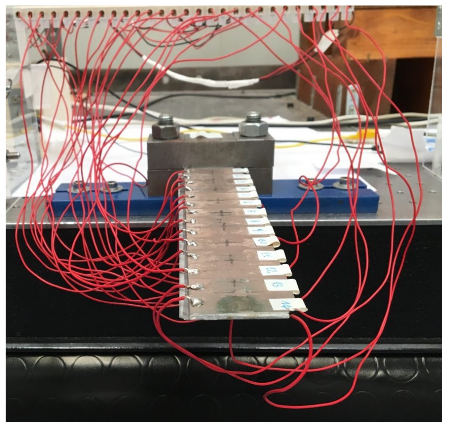
In order to test the model, numerical and experimental investigations were carried out. An experimental workbench was developed and two arrays of 13 PZT plates (PPs) were attached by means of an epoxy glue on both sides of an aluminium alloy cantilever beam. The dimensions of beam and PZT elements are summarized in Table 1, while a picture of the beam coupled with the PPs is shown in Figure 6.
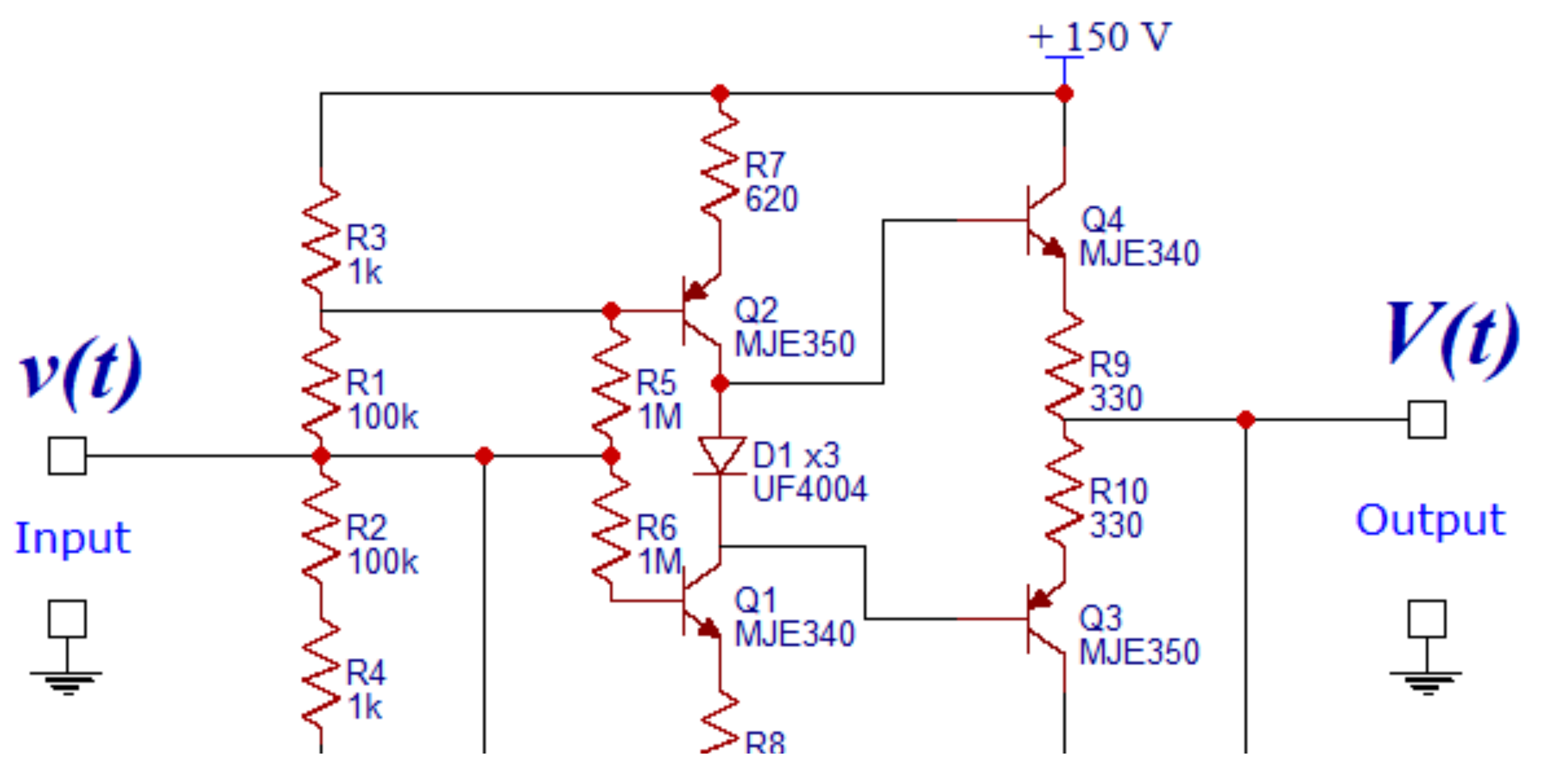
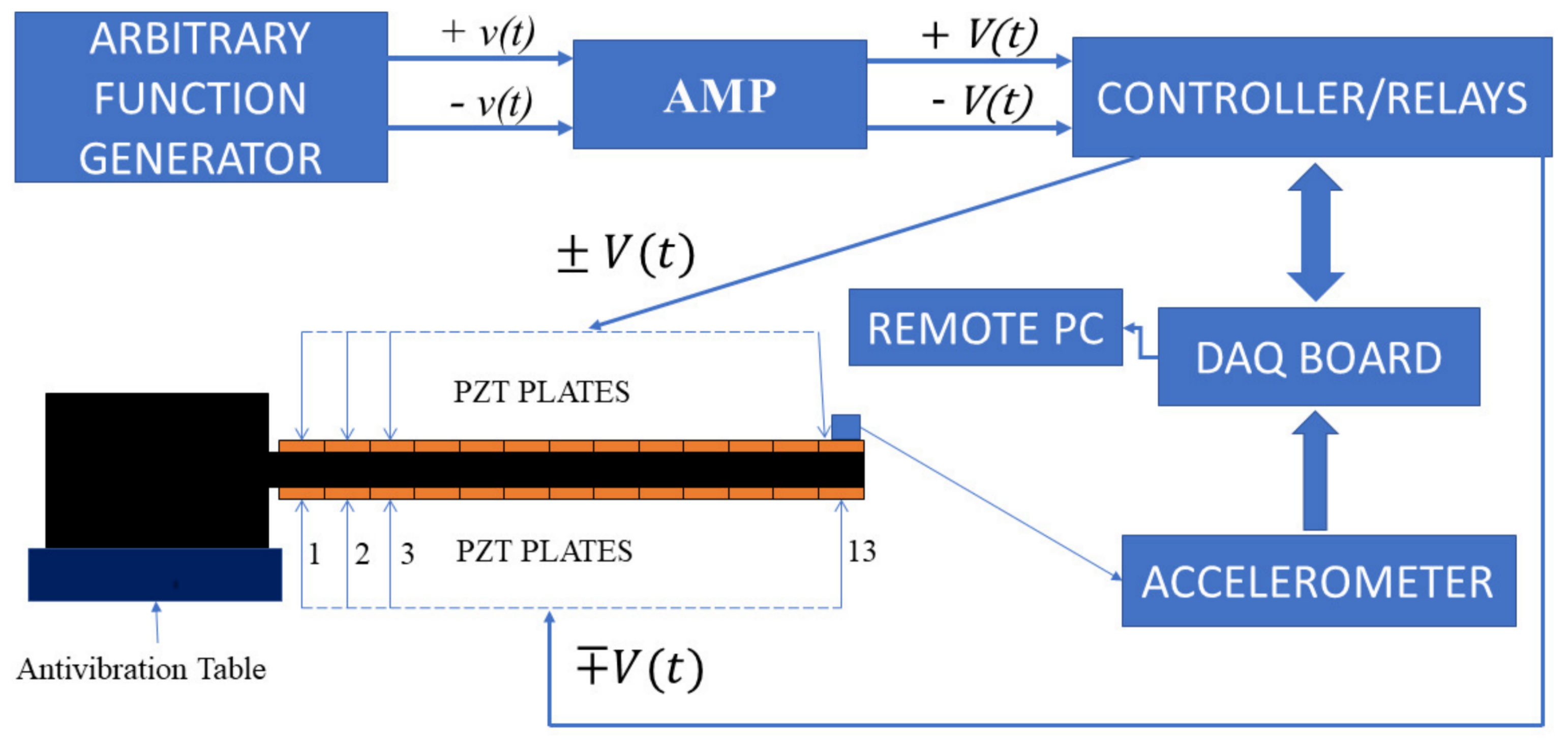
By means of an ad hoc developed power supply circuit, the voltage of Equation (11) is provided to each piezo plate. Every PP is wired to a mechanical relay that is actuated by a micro controller. The relays can switch independently the sign of each PP supply voltage in order to execute a specific PZT activation pattern (i.e., the potential distribution of Table 2. The voltage is provided by an arbitrary function generator (Yokogawa FG420) and properly amplified and inverted by two amplifier circuits specifically developed by the authors. The circuit diagram of the amplifiers is shown in Figure 7 and provides appropriate voltages to actuate the piezoelectric plates. It basically consists of two pairs of complementary transistors (MJE340, MJE350), 10 resistors, and three fast diodes; such a circuit is able to achieve an amplification factor of 10 up to 300 . These features, along with their inexpensiveness and their ease of implementation, make these amplifiers particularly suitable for piezoelectric plate actuation. An ICP micro-accelerometer (PCB 352A56) was placed at the free end of the beam and a data acquisition board (NI USB 6251), and a Labview subroutine was used for collecting and processing the measured data. The sampling rate was set at 15 kHz and 4 s of acceleration was acquired for each PP activation pattern. The FFT analysis of the measured data was performed for each PP activation pattern, so that the amplitudes of the acceleration at and could be assessed. Finally, the total tip displacement was calculated for each PP activation pattern in order to identify the optimal experimental potential distributions of the PPs. The overall measurement chain scheme is illustrated in Figure 8.
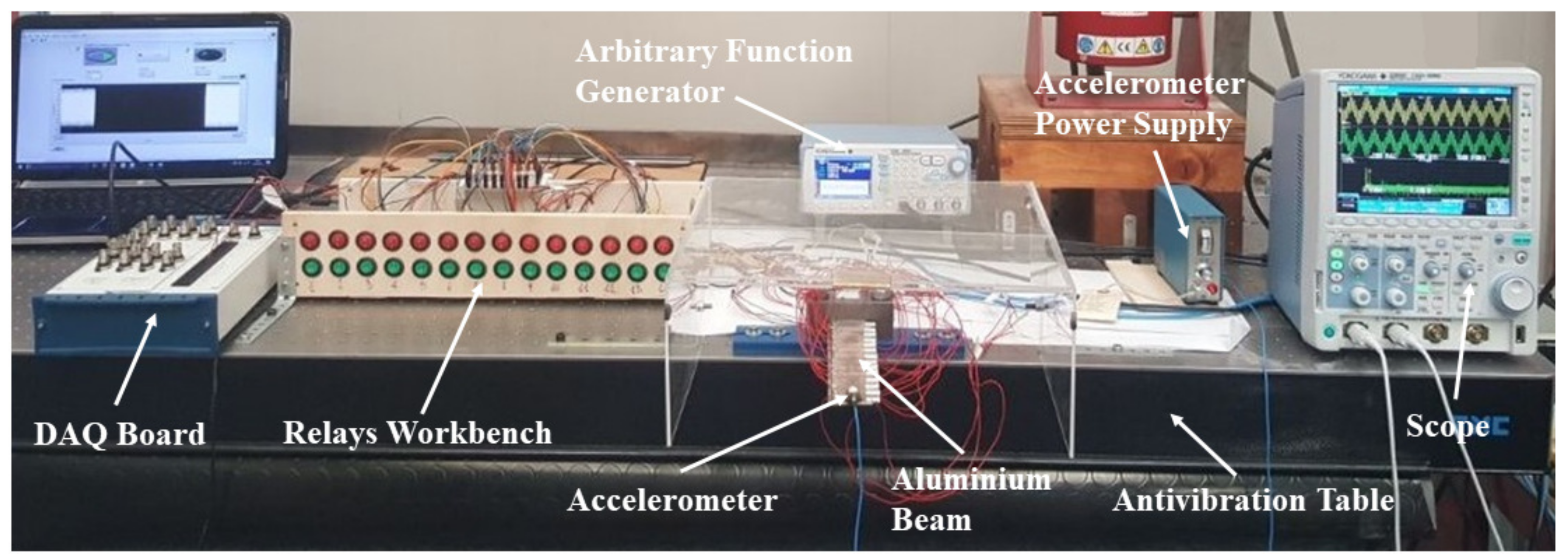
The experimental trials were repeated several times for every PP activation pattern, and four combinations of and were tested. The r ratio (the parameter r takes into account the distribution of the load between the two eigenfrequencies (see Equation (10))) was varied by step of 0.1 from 0 to 1. The actual experimental setup is shown in Figure 9, and its uncertainty (i.e., the accelerometer, the acquisition board, the power supply system, and the data processing) is estimated to be 5% according to previous studies [23,24].
A COMSOL® FEM code was chosen to conduct the numerical simulations. The first four modes, and their pairings, were considered. For every combination (Table 2), and every value of r, the amplitude displacement at the free end of the beam was calculated by the frequency response function. Among all of these, the potential distribution, which implied the maximum amplitude, was considered optimal. The characteristics of the beam and of the piezoelectric elements are reported in Table 1.
4. Results and Discussion
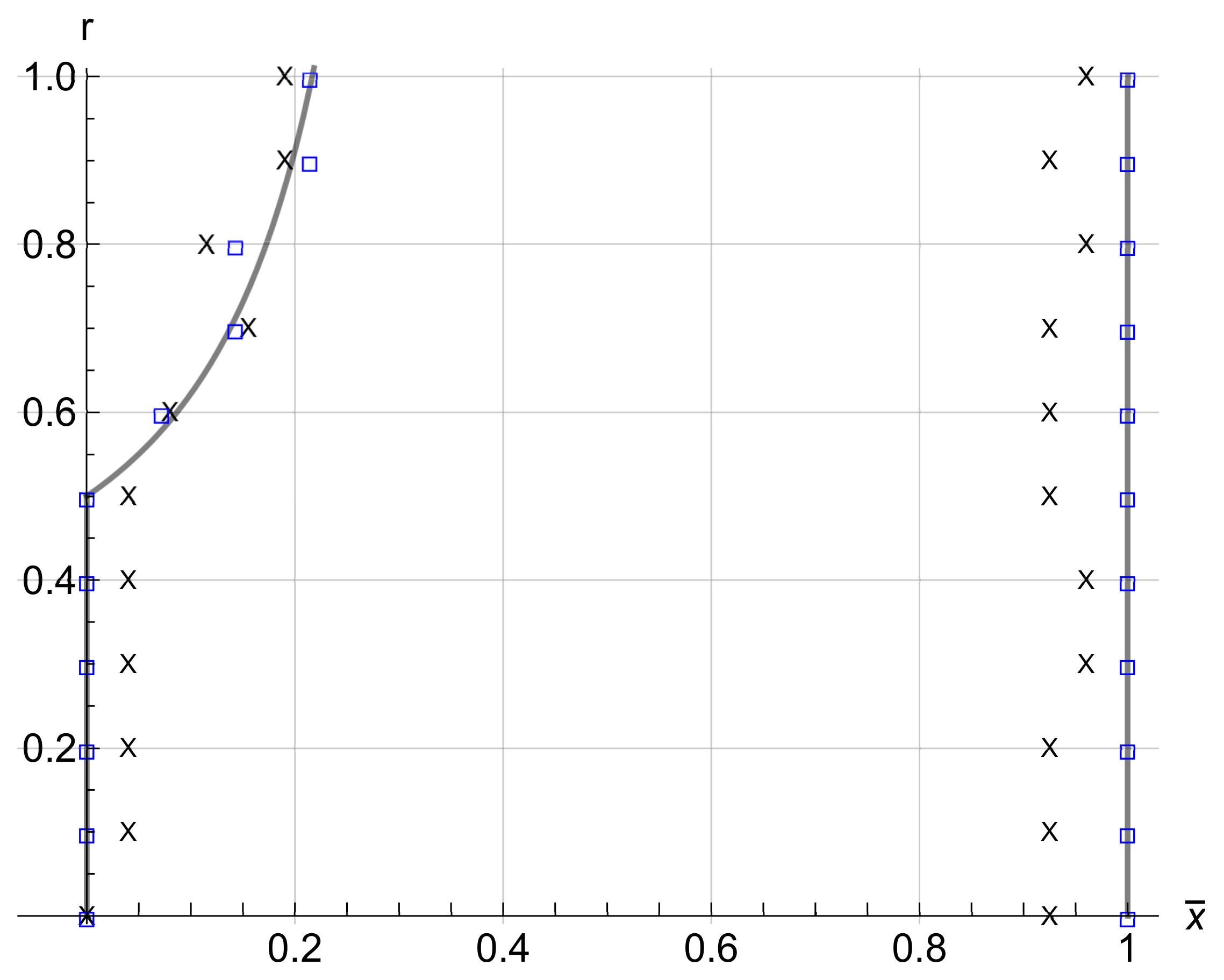
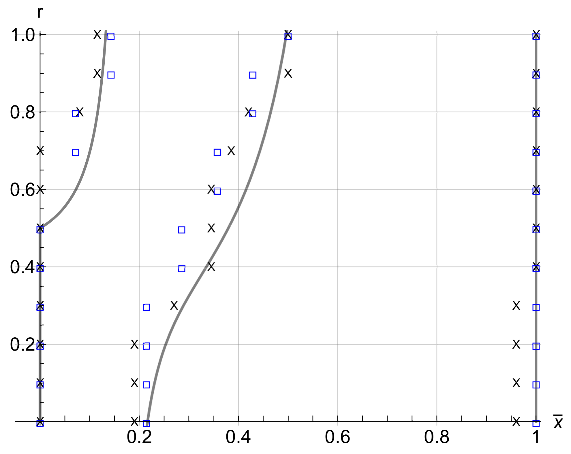
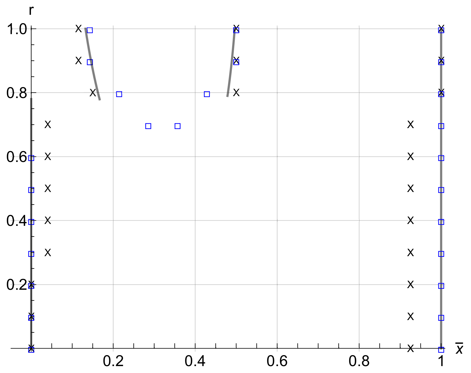
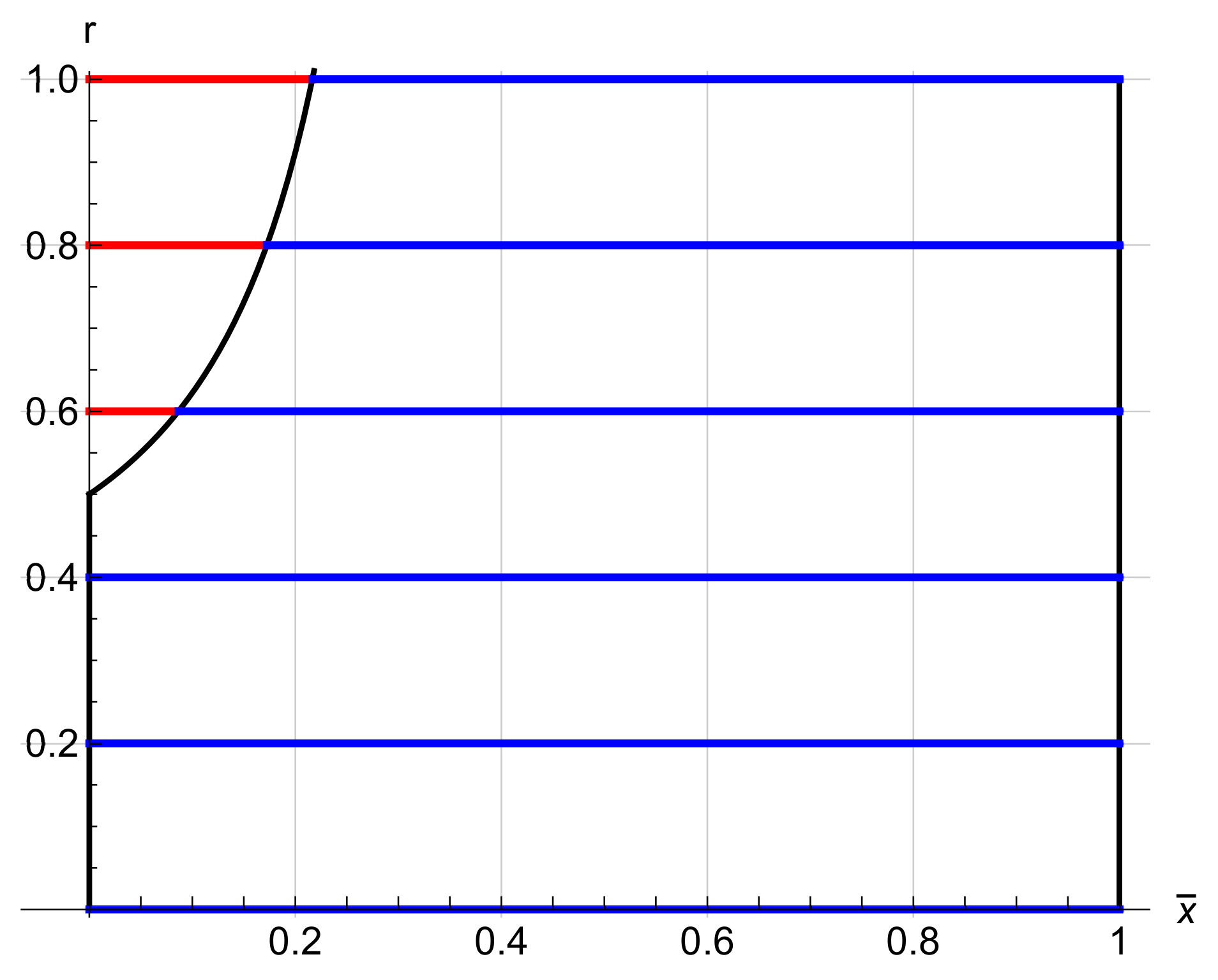
The model, numerical, and experimental results are reported in Figure 10, Figure 11, Figure 12 and Figure 13. It can be observed that there is a good agreement between the numerical and experimental results and those predicted by the model. However, the position evaluation error is due to two principal factors. The first is that the model proposed is a continuum model, which implies that it includes the possibility to change the sign of the potential at every point x. On the other hand, the numerical and experimental simulations inevitably provide a discrete approach, and the sign can be changed only in a discrete number of points. In the specimen piezoelectric coupled beam described above, there are 13 points where the sign can be changed, and these do not always coincide with those provided by the continuum model. In the worst cases, the continuum model points are in the center of one of the 13 couples of the piezoelectric plates. In this case, the error committed is , which is the maximum error within the considered domain. In some cases, this error is larger, but this happens only at the boundary of the domain in for and . The reason for this is due to the shape of and in (Figure 3) and the uncertainty of the measuring equipment (estimated about as described above). In fact, all functions have the first derivative equal to zero in , but and are quite flat for a long interval near . Since the difference in between two different potential combinations is connected with the difference that the assume in these configurations, if this difference is below the , the measuring equipment is not capable of capturing it and the position evaluation error can be considerable (Figure 14). In Figure 10, Figure 11, Figure 12 and Figure 13, it can be observed that, when the modal order number increases the number of the “line changing sign”, the corresponding number of points also increases. In fact, increasing the modal order number increases the number of the extrema of the derivative of the flexural displacement or, in other words, the extrema of the section rotation of the beam (the Euler Bernoulli beam is considered here). Equation (12) shows that the maximum efficiency of the piezoelectric plates is obtained when the sign change occurs in these extrema points. In Figure 15, Figure 16, Figure 17 and Figure 18, some configurations with the potential distribution (lines of the same color represent areas with the same sign) are represented. The increase of with r is due to the fact that, when r rises, the flexural deformation switches from the modal shape to .
5. Conclusions
In this paper, research on the optimal placement of piezoelectric plates for damping flexural vibrations is conjoined with research on the optimal potential distribution. In this way, a more efficient system is obtained, because PZT plates can always work and make a contribution for every combination of loads. In this regard, a new mathematical model, an improvement on an existing method, is proposed. The model outcomes are compared with the results of numerical simulations and experimental data, and a good agreement among them was found. Future works will focus on the implementation of the model in cases of rotating cantilever beams. The interest in these studies could be, e.g., the damping of the blade vibrations in turbomachinery [25,26,27,28].
Author Contributions
Fabio Botta designed and developed the model. Andrea Rossi, Fabio Botta, and Andrea Scorza carried out the experimental tests. Fabio Botta carried out the numerical simulations.
Conflicts of Interest
The authors declare no conflict of interest.
Abbreviations
| B | control vector |
| C | damping matrices |
| piezoelectric coefficient | |
| Young’s modulus of the piezoelectric material | |
| Young’s modulus of the beam | |
| K | stiffness matrices |
| beam length | |
| M | piezoelectric bending moment |
| M | mass matrices |
| r | ratio of the j-th component of the tension |
| piezoelectric thickness | |
| beam thickness | |
| V | voltage applied to the piezoelectric plates |
| w | vertical displacement |
| virtual vertical displacement | |
| damping coefficient | |
| i-th flexural mode of the cantilever beam | |
| adimensional length of the beam: | |
| points where the potential changes its sign | |
| natural frequency |
References
- Poursaeidi, E.; Salavatian, M. Fatigue grow simulation in a generator fan blade. Eng. Fail. Anal. 2009, 16, 888–898. [Google Scholar] [CrossRef]
- Witek, L. Experimental crack propagation and failure analysis of the first stage compressor blade subject to vibration. Eng. Fail. Anal. 2009, 16, 2163–2170. [Google Scholar] [CrossRef]
- Kubiac, S.J.; Urquiza, G.B.; Garcia, C.J.; Sierra, E.F. Failure analysis of steam turbine last stage blade tenon and shroud. Eng. Fail. Anal. 2007, 14, 1476–1487. [Google Scholar] [CrossRef]
- Motta, V.; Malzacher, L.; Peitsch, D. Numerical Assessment of Virtual Control Surfaces for Load Alleviation on Compressor Blades. Appl. Sci. 2018, 8, 125. [Google Scholar] [CrossRef]
- Yan, B.; Wang, K.; Hu, Z.; Wu, C.; Zhang, X. Shunt Damping Vibration Control Technology: A Review. Appl. Sci. 2017, 7, 494. [Google Scholar] [CrossRef]
- Guo, K.; Xu, Y. Random Vibration Suppression of a Truss Core Sandwich Panel Using Independent Modal Resonant Shunt and Modal Criterion. Appl. Sci. 2017, 7, 496. [Google Scholar] [CrossRef]
- Crawley, E.F.; de Luis, J. Use of piezoelectric actuators as elements of intelligent structures. AIAA J. 1987, 25, 1373–1385. [Google Scholar] [CrossRef]
- Kim, B.; Yoon, J.-Y. Enhanced Adaptive Filtering Algorithm Based on Sliding Mode Control for Active Vibration Rejection of Smart Beam Structures. Appl. Sci. 2017, 7, 750. [Google Scholar] [CrossRef]
- Lou, J.; Liao, J.; Wei, Y.; Yang, Y.; Li, G. Experimental Identification and Vibration Control of A Piezoelectric Flexible Manipulator Using Optimal Multi-Poles Placement Control. Appl. Sci. 2017, 7, 309. [Google Scholar] [CrossRef]
- Frecker, M.I. Recent Advances in Optimization of Smart Structures and Actuators. J. Intell. Mater. Syst. Sruct. 2003, 14, 207–216. [Google Scholar] [CrossRef]
- Gupta, V.; Sharma, M.; Nagesh, T. Optimization Criteria for Optimal Placement of Piezoelectric Sensors and Actuators on a Smart Structure: A Technical Review. J. Intell. Mater. Syst. Sruct. 2010, 21, 1227–1243. [Google Scholar] [CrossRef]
- Dhuri, K.D.; Seshu, P. Piezo actuator placement and sizing for good control effectiveness and minimal change in original system dynamics. Smart Mater. Struct. 2006, 15, 1661–1672. [Google Scholar] [CrossRef]
- Kumar, K.R.; Narayanan, S. Active vibration control of beams with optimal placement of piezoelectric sensor/actuator pairs. Smart Mater. Struct. 2008, 17, 055008. [Google Scholar] [CrossRef]
- Demetriou, M.A. A Numerical Algorithm for the Optimal Placement of Actuators and Sensors for Flexible Structures. In Proceedings of the American Control Conference, Chicago, IL, USA, 28–30 June 2000; pp. 2290–2294. [Google Scholar]
- Bruant, I.; Coffignal, G.; Lene, F.; Verge, M. A methodology for determination of piezoelectric actuator and sensor location on beam structures. J. Sound Vib. 2001, 245, 861–882. [Google Scholar] [CrossRef]
- Sunar, M.; Rao, S.S. Distribuited Modeling and Actuator Location for Piezoelectric Control System. AIAA J. 1996, 34, 2209–2211. [Google Scholar] [CrossRef]
- Yang, Y.; Zhanli, J.; Soh, C.K. Integrated optimal design of vibration control system for smart beams using genetic algorithms. J. Sound Vib. 2005, 119, 487–508. [Google Scholar] [CrossRef]
- Barboni, R.; Mannini, A.; Fantini, E.; Gaudenzi, P. Optimal placement of PZT actuators for the control of beam dynamics. Smart Mater. Struct. 2000, 9, 110–120. [Google Scholar] [CrossRef]
- Aldraihem, O.J.; Singh, T.; Wetherhold, R.C. Optimal Size and Location of Piezoelectric Actuator/Sensors: Practical Considerations. J. Guid. Control Dyn. 2000, 23, 509–515. [Google Scholar] [CrossRef]
- Baz, A.; Poh, S. Performance of an active control system with piezoelectric actuators. J. Sound Vib. 1988, 126, 327–343. [Google Scholar] [CrossRef]
- Wang, Q.; Wang, C.M. Optimal placement and size of piezoelectric patches on beams from the controllability perspective. Smart Mater. Struct. 2000, 9, 558–567. [Google Scholar] [CrossRef]
- Botta, F.; Dini, D.; Schwingshackl, C.; di Mare, L.; Cerri, G. Optimal Placement of Piezoelectric Plates to Control Multimode Vibrations of a Beam. Adv. Acoust. Vib. 2013, 2013. [Google Scholar] [CrossRef]
- Rossi, A.; Orsini, F.; Scorza, A.; Botta, F.; Sciuto, S.A.; Di Giminiani, R. A preliminary characterization of a whole body vibration platform prototype for medical and rehabilitation application. In Proceedings of the 2016 IEEE International Symposium on Medical Measurements and Applications (MeMeA), Benevento, Italy, 15–18 May 2016. art. no. 7533721. [Google Scholar]
- Rossi, A.; Orsini, F.; Scorza, A.; Botta, F.; Sciuto, S.A.; Di Giminiani, R. A preliminary uncertainty analysis of acceleration and displacement measurements on a novel WBV platform for biologic response studies. In Proceedings of the 2016 IEEE International Symposium on Medical Measurements and Applications (MeMeA), Benevento, Italy, 15–18 May 2016. art. no. 7533722. [Google Scholar]
- Hohl, A.; Neubauer, M.; Schwarzendahl, S.M.; Panning, L.; Wallaschek, J. Active and semiactive Vibration Damping of Turbine Blades with Piezoceramics. Proc. SPIE 2009, 7288, 72881H1–72881H10. [Google Scholar]
- Goltz, I.; Bohmer, H.; Nollau, R.; Belz, J.; Grueber, B.; Seume, J.R. Piezo-electric actuation of rotor blades in an axial compressor with Piezoceramics. In Proceedings of the 8th European Conference on Turbomachinery (ETC), Graz, Austria, 23–27 March 2009. [Google Scholar]
- Provenza, A.J.; Morrison, C.R. Control of fan blade vibrations using piezoelectric and bi-directional telemetry. In Proceedings of the ASME Turbo Expo, Vancouver, BC, Canada, 6–10 June 2011. [Google Scholar]
- Lin, S.M.; Lin, J.M. Vibration of Rotating Smart Beam. AIAA J. 2007, 4, 382–389. [Google Scholar] [CrossRef]
Figure 1.
The piezoelectric coupled beam.

Figure 2.
Actions of the piezoelectric plate on the beam.
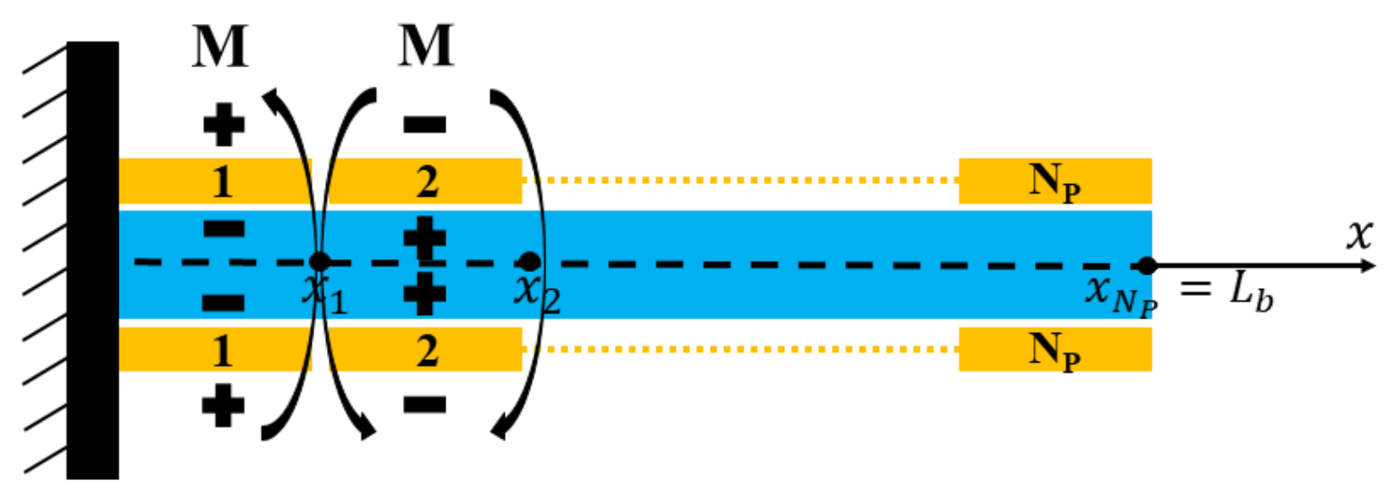
Figure 3.
The functions for different combinations of the first four eigenmodes. grey: r = 0.0; brown: r = 0.2; blue: r = 0.4; purple: r = 0.6; orange: r = 0.8; green: r = 1.0; black: extrema line points.
Figure 3.
The functions for different combinations of the first four eigenmodes. grey: r = 0.0; brown: r = 0.2; blue: r = 0.4; purple: r = 0.6; orange: r = 0.8; green: r = 1.0; black: extrema line points.

Figure 4.
—the optimal potential distribution for coupling between the first two modes.
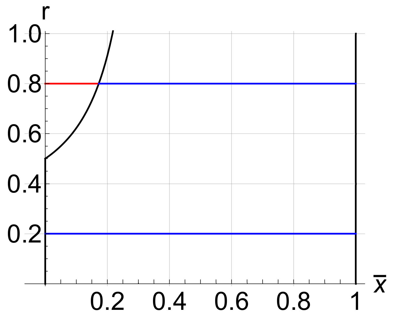
Figure 5.
—the optimal potential distribution for and .

Figure 6.
A detail of the aluminium beam coupled with two arrays of 13 PZT plates (PPs).

Figure 7.
Measurement chain and experimental workbench functional scheme.

Figure 8.
The authors’ amplifier circuit that drives the piezoelectric plates (the resistances are expressed in ).
Figure 8.
The authors’ amplifier circuit that drives the piezoelectric plates (the resistances are expressed in ).

Figure 9.
Experimental setup.

Figure 10.
Coupling between the first and second modes. ![Applsci 08 00551 i001]() = model solution; = FEM simulations; × = experimental results.
= model solution; = FEM simulations; × = experimental results.
 = model solution; = FEM simulations; × = experimental results.
Figure 10.
Coupling between the first and second modes. ![Applsci 08 00551 i001]() = model solution; = FEM simulations; × = experimental results.
= model solution; = FEM simulations; × = experimental results.
= model solution; = FEM simulations; × = experimental results.
Figure 11.
Coupling between the second and third modes. ![Applsci 08 00551 i001]() = model solution; = FEM simulations; × = experimental results.
= model solution; = FEM simulations; × = experimental results.
= model solution; = FEM simulations; × = experimental results.
Figure 11.
Coupling between the second and third modes. ![Applsci 08 00551 i001]() = model solution; = FEM simulations; × = experimental results.
= model solution; = FEM simulations; × = experimental results.
= model solution; = FEM simulations; × = experimental results.
Figure 12.
Coupling between the third and fourth modes. ![Applsci 08 00551 i001]() = model solution; = FEM simulations; × = experimental results.
= model solution; = FEM simulations; × = experimental results.
= model solution; = FEM simulations; × = experimental results.
Figure 12.
Coupling between the third and fourth modes. ![Applsci 08 00551 i001]() = model solution; = FEM simulations; × = experimental results.
= model solution; = FEM simulations; × = experimental results.
= model solution; = FEM simulations; × = experimental results.
Figure 13.
Coupling between the first and third modes. ![Applsci 08 00551 i001]() = model solution; = FEM simulations; × = experimental results.
= model solution; = FEM simulations; × = experimental results.
= model solution; = FEM simulations; × = experimental results.
Figure 13.
Coupling between the first and third modes. ![Applsci 08 00551 i001]() = model solution; = FEM simulations; × = experimental results.
= model solution; = FEM simulations; × = experimental results.
= model solution; = FEM simulations; × = experimental results.
Figure 14.
Uncertainty of the position due to error in the measuring equipment.
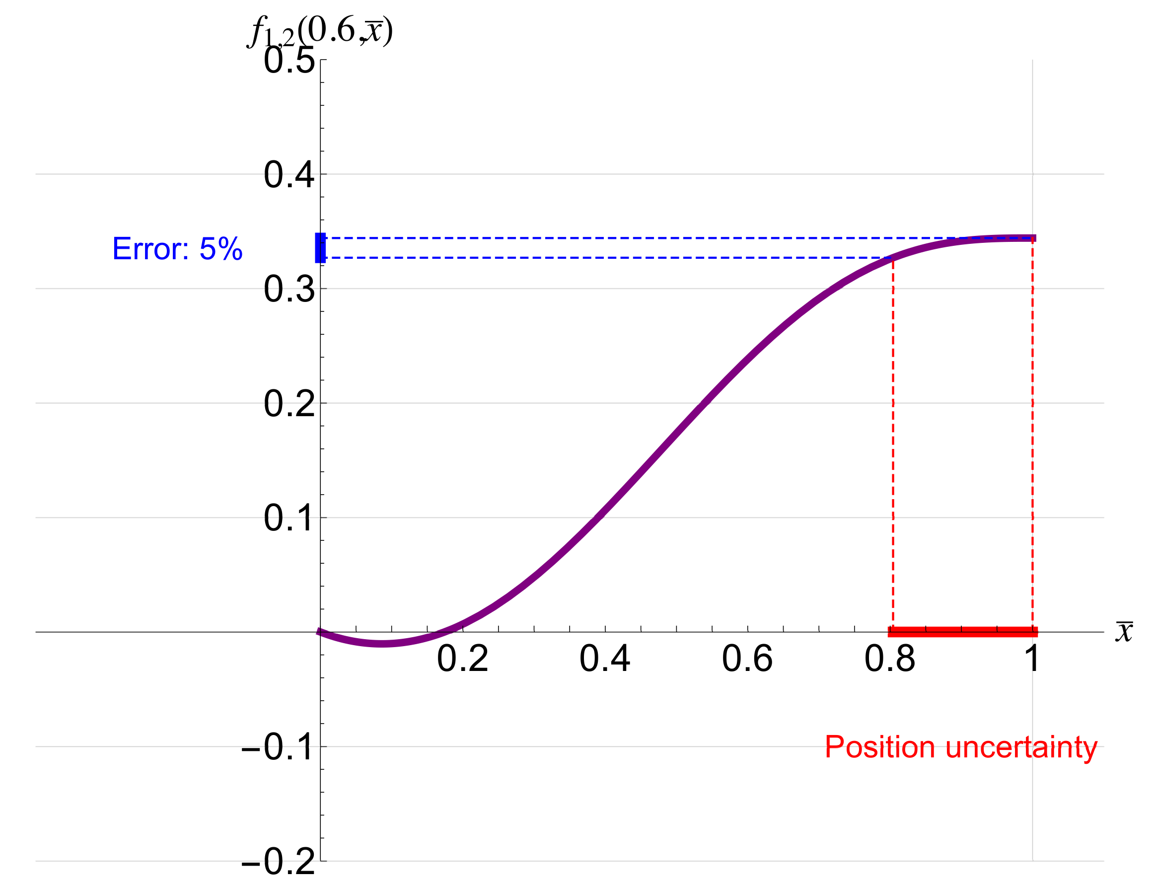
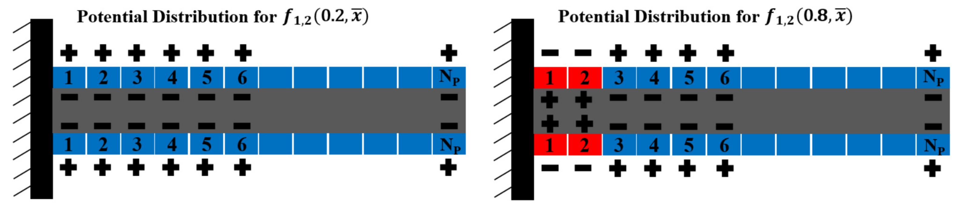
Figure 15.
Potential distribution when there is a coupling between the first and second modes.

Figure 16.
Potential distribution when there is a coupling between the second and third modes.
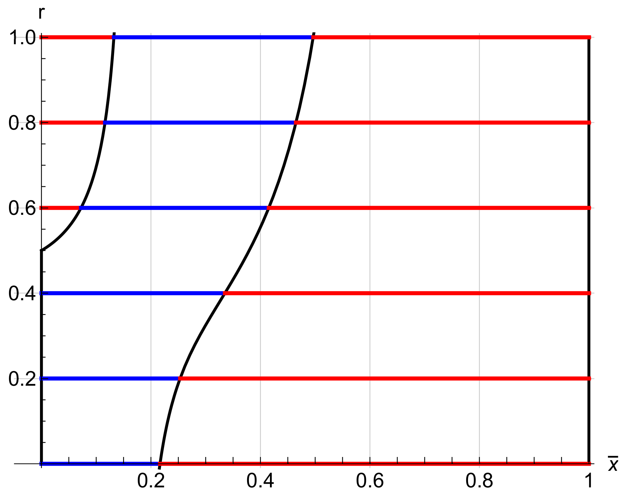
Figure 17.
Potential distribution when there is a coupling between the third and fourth modes.

Figure 18.
Potential distribution when there is a coupling between the first and third modes.

Table 1.
Cantilever beam and lead zirconate titanate (PZT) plate specifications, and lengths are expressed in mm.
Table 1.
Cantilever beam and lead zirconate titanate (PZT) plate specifications, and lengths are expressed in mm.
| Material | Length | Width | Thickness | |
|---|---|---|---|---|
| Beam | Aluminium | 185 | 36 | 1.5 |
| PZT plate | PIC 255 (PI Ceramic) | 40 | 14 | 0.5 |
Table 2.
Combinations of the potential distribution.
| Combination\Plates Couple | 1 | 2 | 3 | 4 | 5 | 6 | 7 | 8 | 9 | 10 | 11 | 12 | 13 |
|---|---|---|---|---|---|---|---|---|---|---|---|---|---|
| 1 | +1 | +1 | +1 | +1 | +1 | +1 | +1 | +1 | +1 | +1 | +1 | +1 | +1 |
| 2 | +1 | +1 | +1 | +1 | +1 | +1 | +1 | +1 | +1 | +1 | +1 | +1 | −1 |
| 3 | +1 | +1 | +1 | +1 | +1 | +1 | +1 | +1 | +1 | +1 | +1 | −1 | +1 |
| 4 | +1 | +1 | +1 | +1 | +1 | +1 | +1 | +1 | +1 | +1 | +1 | −1 | −1 |
| 5 | +1 | +1 | +1 | +1 | +1 | +1 | +1 | +1 | +1 | +1 | −1 | +1 | +1 |
| ... | ... | ... | ... | ... | ... | ... | ... | ... | ... | ... | ... | ... | ... |
| −1 | −1 | −1 | −1 | −1 | −1 | −1 | −1 | −1 | −1 | −1 | −1 | −1 |
© 2018 by the authors. Licensee MDPI, Basel, Switzerland. This article is an open access article distributed under the terms and conditions of the Creative Commons Attribution (CC BY) license (http://creativecommons.org/licenses/by/4.0/).
Share and Cite
MDPI and ACS Style
Botta, F.; Scorza, A.; Rossi, A. Optimal Piezoelectric Potential Distribution for Controlling Multimode Vibrations. Appl. Sci. 2018, 8, 551. https://doi.org/10.3390/app8040551
AMA Style
Botta F, Scorza A, Rossi A. Optimal Piezoelectric Potential Distribution for Controlling Multimode Vibrations. Applied Sciences. 2018; 8(4):551. https://doi.org/10.3390/app8040551
Chicago/Turabian StyleBotta, Fabio, Andrea Scorza, and Andrea Rossi. 2018. "Optimal Piezoelectric Potential Distribution for Controlling Multimode Vibrations" Applied Sciences 8, no. 4: 551. https://doi.org/10.3390/app8040551
Note that from the first issue of 2016, this journal uses article numbers instead of page numbers. See further details here.