A Hybrid Metaheuristic for Multi-Objective Scientific Workflow Scheduling in a Cloud Environment

1
School of Computer Science and Engineering, South China University of Technology, Guangzhou 510006, China
2
Department of Computer Science, University of Education, Lahore 54770, Pakistan
*
Author to whom correspondence should be addressed.
Appl. Sci. 2018, 8(4), 538; https://doi.org/10.3390/app8040538
Submission received: 27 February 2018
/
Revised: 22 March 2018
/
Accepted: 28 March 2018
/
Published: 31 March 2018
Abstract
:Cloud computing has emerged as a high-performance computing environment with a large pool of abstracted, virtualized, flexible, and on-demand resources and services. Scheduling of scientific workflows in a distributed environment is a well-known NP-complete problem and therefore intractable with exact solutions. It becomes even more challenging in the cloud computing platform due to its dynamic and heterogeneous nature. The aim of this study is to optimize multi-objective scheduling of scientific workflows in a cloud computing environment based on the proposed metaheuristic-based algorithm, Hybrid Bio-inspired Metaheuristic for Multi-objective Optimization (HBMMO). The strong global exploration ability of the nature-inspired metaheuristic Symbiotic Organisms Search (SOS) is enhanced by involving an efficient list-scheduling heuristic, Predict Earliest Finish Time (PEFT), in the proposed algorithm to obtain better convergence and diversity of the approximate Pareto front in terms of reduced makespan, minimized cost, and efficient load balance of the Virtual Machines (VMs). The experiments using different scientific workflow applications highlight the effectiveness, practicality, and better performance of the proposed algorithm.
1. Introduction
Cloud computing has emerged as an effective distributed computing utility which may be used for deploying large and complex scientific workflow applications [1,2]. Workflows decompose complex, data-intensive applications into smaller tasks and execute those tasks in serial or parallel depending on the nature of the application. A workflow application is represented graphically using a Directed Acyclic Graph (DAG) to reflect the interdependencies among the workflow’s tasks, where the nodes represent computational tasks of the workflow and the directed edges between the nodes determine data dependencies (that is, data transfers), control dependencies (that is, order of execution), and precedence requirements between the tasks. However, resource allocation and scheduling of tasks of a given workflow in a cloud environment are issues of great importance.
Optimization of workflow scheduling is an active research area in the Infrastructure as a Service (IaaS) cloud. It is an NP-complete problem, so building an optimum workflow scheduler with reasonable performance and computation speed is very challenging in the heterogeneous distributed environment of clouds [3].
A Multi-objective Optimization Problem (MOP) is characterized by multiple conflicting objectives that require simultaneous optimization. Unlike single objective optimization, there is no single feasible solution that optimizes all objective functions; instead, a set of non-dominated solutions with optimal trade-offs known as Pareto optimal solutions can be found for MOPs. The set of all Pareto optimal solutions in the objective space is called the Pareto front [4]. Many existing studies deal with cloud workflow scheduling as a single or bi-objective optimization problem without considering some important requirements of the users or the providers. Therefore, it is highly desirable to formulate scheduling of the workflow applications as a MOP taking into account the requirements from the user and the service provider. For example, the cloud workflow scheduler might wish to consider user’s Quality of Service (QoS) objectives, such as makespan and cost, as well as provider’s objectives, such as efficient load balancing over the Virtual Machines (VMs).
Predict Earliest Finish Time (PEFT) [5] is an efficient heuristic in terms of makespan proposed for task scheduling in heterogeneous systems. This heuristic assign priorities to tasks and schedules them in a priority order to the known-best VM. However, list-based heuristics are only locally optimal. Therefore, a metaheuristic approach can be very effective to achieve better optimization solutions for workflow scheduling in the cloud. However, each metaheuristic algorithm has its own merits and demerits. Therefore, hybrid approaches have shown to produce better results [6,7] as they combine heuristic rules with metaheuristic algorithms and have attracted much attention in recent years to solve multi-objective workflow scheduling problems in the cloud.
Symbiotic Organisms Search (SOS) [8] was proposed as a nature-inspired metaheuristic optimization algorithm that was inspired by the interactive behavior between organisms in an ecosystem to live together and survive. SOS is a simply structured, powerful, easy to use, and robust algorithm for solving global optimization problems. The SOS algorithm has strong global exploration, faster convergence capability, and requires only common controlling parameters, such as population size and initialization. Recently, a discrete version of SOS [9] was proposed for scheduling a bag of tasks in the cloud environment.
This paper proposes a hybrid metaheuristic for multi-objective workflow scheduling in a cloud based on the list-based heuristic algorithm PEFT and the discrete version of the metaheuristic algorithm SOS to achieve optimum convergence and diversity of the Pareto front. The two conflicting objectives of the proposed scheme Hybrid Bio-inspired Metaheuristic for Multi-objective Optimization (HBMMO) are to minimize makespan and to reduce cost along with the efficient utilization of the VMs. Therefore, the proposed multi-objective approach based on a Pareto optimal non-dominated solution considers the users’ as well as providers’ requirements for workflow scheduling in the cloud.
The remaining sections of the paper are organized as follows. Section 2 discusses the background and investigates related work in the recent literature. Section 3 presents the system model and the problem formulation of the proposed method. After that, Section 4 describes the proposed algorithm. Then, the results of a simulation and its analysis are discussed in Section 5. Finally, Section 6 presents the main conclusions of the study.
2. Related Work
Several heuristic and metaheuristic algorithms have tried to address workflow scheduling in the cloud environment using different strategies [10,11,12,13,14]. Critical Path On a Processor (CPOP), Heterogeneous Earliest Finish Time (HEFT) [10], Heterogeneous Critical Parent Trees (HCPT), High Performance Task Scheduling (HPS), Performance Effective Task Scheduling (PETS), Lookahead, and PEFT [5] are some of the well-known list-based scheduling heuristics. All of them attempt to find suitable schedule maps on the basis of some pre-defined rules and problem size. Hence, they are only locally optimal and infeasible for large and complex workflow scheduling problems in the cloud. Recently, Anwar and Deng (2018) [15] proposed a model, Dynamic Scheduling of Bag of Tasks based workflows (DSB), for scheduling large and complex scientific workflows on elastic, heterogeneous, scalable, and dynamically provisioned VMs. It minimizes the financial cost under a deadline constraint. However, all of them consider the optimization of a single objective only.
The metaheuristic-based techniques are used to find near-optimal solutions for these complex workflow scheduling problems. Recently, a number of nature-inspired metaheuristic-based techniques, such as Artificial Bee Colony (ABC), Ant Colony Optimization (ACO), the Bat Algorithm (BA), Cuckoo Search (CS), Differential Evolution (DE), the Firefly Algorithm (FA), the Genetic Algorithm (GA), Harmony Search (HS), the Immune Algorithm (IA), the League Championship Algorithm (LCA), the Lion Optimization Algorithm (LOA), the Memetic Algorithm (MA), Particle Swarm Optimization (PSO), and Simulated Annealing (SA) [16] have been applied in solving the task scheduling problem.
A metaheuristic algorithm can be improved in terms of the quality of the solution or convergence speed by combining it with another population-based metaheuristic algorithm or some local search-based metaheuristic algorithm [17]. Domanal et al. (2017) [18] proposed a hybrid bio-inspired algorithm for task scheduling and resource management of cloud resources in terms of efficient resource utilization, improved reliability, and reduced average response time. Pooranian et al. (2015) [19] hybridized a gravitational emulation local search strategy with particle swarm optimization to improve the obtained solution. Abdullahi and Ngadi (2016) [20] proposed an SA-based SOS in order to improve the convergence rate and quality of solution.
The MOP is a very promising direction to tackle the problem of workflow scheduling in the cloud. Zhang (2014) [21] used the MOP approach based on a Pareto optimal non-dominated solution for the workflow scheduling problem in the cloud. Zhu et al. (2016) [2] proposed an evolutionary multi-objective scheduling for cloud (EMS-C) algorithm to solve the workflow scheduling problem on the IaaS platform. Extensions of HEFT [10], the Pareto Optimal Scheduling Heuristic (POSH) [22], and Multi-Objective Heterogeneous Earliest Finish Time (MOHEFT) [3] were designed to provide users with a set of trade-off optimal solutions for scheduling workflows in the cloud. A multi-objective heuristic algorithm, Min-min based time and cost tradeoff (MTCT), was proposed by Xu et al. (2016) [23]. A scheduling approach, the Balanced and file Reuse-Replication Scheduling (BaRRS) algorithm, was proposed to select the optimal solution based on makespan and cost [24]. However, they focus on only two objectives.
Recently, some hybrid multi-objective algorithms have been used by combining the good features of two or more approaches: adaptive hybrid PSO [25], the hybrid multi-objective population migration algorithm [26], Multi-Objective SOS (MOSOS) with an adaptive penalty function [27], non-dominance sort-based Hybrid PSO (HPSO) [28], and Fragmentation-Based Genetic Algorithm (FBGA) [29]. Although there has been considerable research conducted on Pareto-based optimal methods [30,31,32], further study is needed to enhance the convergence and diversity of the approximate Pareto front in the context of cloud computing.
3. Problem Description for the Proposed Methodology
Table 1 summarizes important notations and their definitions used throughout this paper.
3.1. System Model
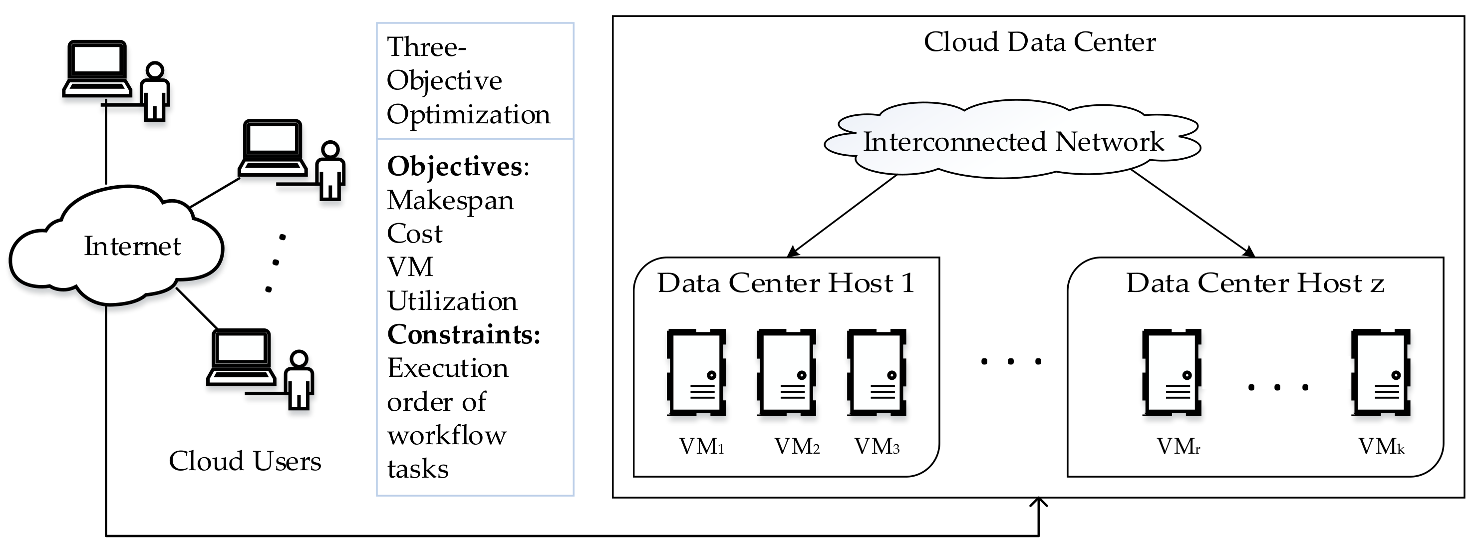
The cloud data center used in this study is represented by a set of heterogeneous VMs, where such that , as shown in Figure 1. Each VM has its own processing speed measured in Millions of Instruction Per Second (MIPS), memory in Megabytes (MB), storage space in MB, bandwidth in Megabits per second (Mbps), and cost per unit of time.
Tasks of scientific workflow applications can be represented by a DAG, , where is the set of vertices representing different tasks of the workflow, and is the set of directed edges between the vertices representing dependencies and precedence constraints. An edge between the tasks and , indicates the precedence constraint that the task cannot start its execution before finishes and sends all the needed output data to task . In this case, task is considered one of the immediate predecessors of task , and task is considered one of the immediate successors of task . Task can have multiple predecessor and multiple successor tasks, denoted as and of , respectively. A task is considered as a ready task when all its predecessors have finished execution. Each task is assumed to have a workload, denoted by , which is the runtime of the task on a specific VM type. Also, each edge has a weight that indicates the data transfer size of the output data from to , denoted by . Any task without a predecessor task is called the entry task , and a task with no successor task is called the exit task , i.e., and respectively. In this work, we assume that the given workflow has single and . So, if a given workflow has more than one entry or exit task, then a virtual or task with , , , , , and is added to the DAG.
3.2. Assumptions
The current study considers the following assumptions similar to the work presented by Anwar and Deng (2018) [15].
- (1)
- The workflow application is assumed to be executed in a single cloud data center, so that one possible source of execution delay, storage cost, and data transmission cost between data centers is eliminated.
- (2)
- An on-demand pricing model is considered, where any partial utilization of the leased VM is charged as a full time period.
- (3)
- The communication time for the tasks executed on the same VM is assumed to be zero.
- (4)
- The scheduling of tasks is considered to be non-preemptive, which means that a task cannot be interrupted while being executed until it has completed its execution.
- (5)
- Each task can be assigned to a single VM, and a VM can process several tasks.
- (6)
- Multi-tenant scenarios are not considered, i.e., each VM can only run one task at a time.
- (7)
- The processing capacity of a VM is provided either from the IaaS provider or can be calculated based on the work reported by Ostermann et al. (2010) [33]. The estimation times are scaled by the processing capacity of VM instances, i.e., 1 s of each task in a workflow runs for 1 s on a VM instance with one Elastic Compute Unit (ECU). Note that an ECU is the central processing unit (CPU) performance unit defined by Amazon. The processing capacity of an ECU (based on [email protected] GHz performing 4 flops per Hz) was estimated at 4.4 GFLOPS (Giga Floating Point Operations Per Second) [33].
- (8)
- When a VM is leased, a boot time of 97 seconds for proper initialization is considered based on the measurements reported by Mao and Humphrey (2011) [34] for the Amazon EC2 cloud.
- (9)
3.3. Multi-Objective Optimization
A MOP has multiple conflicting objectives which need to be optimized simultaneously. Therefore, the goal is to find good trade-off solutions that represent the best possible compromises among the objectives. A MOP problem can be formulated as:
subject to
wherein represents the decision space. consist of objective functions. Since multi-objective optimization usually involve conflicting objectives, so there is no single solution which can optimize all objectives simultaneously. Hence, the desired solution is considered to be any possible solution which is optimal for one or more objectives. For this purpose, the concept of Pareto dominance is mostly employed. Given two solutions , solution Pareto dominates or Pareto dominates if and only if,
where is the th objective function of solution in dimensional space. A solution is denoted as Pareto optimal if and only if such that Pareto dominates , that is, it is not dominated by any other solution within the decision space. The set of all Pareto optimal solutions is termed as the Pareto set and its image in the objective space is called the Pareto front. Workflow scheduling in the cloud can be seen as a MOP whose goal is to find a set of good trade-off solutions enabling the user to select the desired trade-off amongst the objectives.
3.4. Problem Formulation
The objectives of the proposed work are to minimize the makespan, cost, and degree of imbalance among the VMs. In the workflow scheduling problem, the fitness of a solution is the trade-off between the three objectives.
The cloud workflow scheduling problem can be formulated as follows:
subject to
The fitness function is defined by Equations (3)–(6), where , , and indicate minimizing the three objectives, namely makespan, cost, and degree of imbalance among the VMs, respectively. Equation (7) indicates that the makespan of a workflow depends on the finish time of the exit task. Equation (8) defines the execution time of task on VM considering the VM’s performance variability which represent the potential uncertainties, variation, or degradation in CPU performance and network resources due to the multi-tenant, heterogeneous, shared, and virtualized nature of real cloud environments. In other words, it is the amount by which the speed of a VM may degrade. Ultimately, it may result in a degradation in execution time of tasks. Equation (9) calculates the communication time between the tasks and , which represents the ratio of data transfer size from task to to the smallest bandwidth between the VMs and . and are VMs on which and are executed, respectively. When successive tasks execute on the same VM, . Equation (10) represents the start time () of task to be executed on VM . It is computed based on the available time of the VM () for the execution of the task, the maximum value of the sum of the finish time of all its predecessors, and the communication time between its predecessors and itself. After is decided to run on , will be updated as the finish time of the immediate predecessor task that has been executed on the same VM. Specifically, when is the entry task of the application, the start time can be computed as the available time of VM where is mapped during resource allocation. The finish time () of task executed on VM is defined by Equation (11). The total execution cost for the workflow is defined in Equation (12). Equation (13) ensures the precedence constraint that a task can only start execution after its predecessor task has finished and all the required input data is received. Equation (14) measures the degree of imbalance of all leased VMs based on the Euclidean distance. Obviously, minimizing this value will result in higher utilization of VMs. Equation (15) defines the utilization rate of VM . Equation (16) ensures that a task can be assigned to exactly one VM and can be executed only once. Equation (17) guarantees that a task cannot be interrupted while being executed until it has completed its execution.
4. Proposed Work
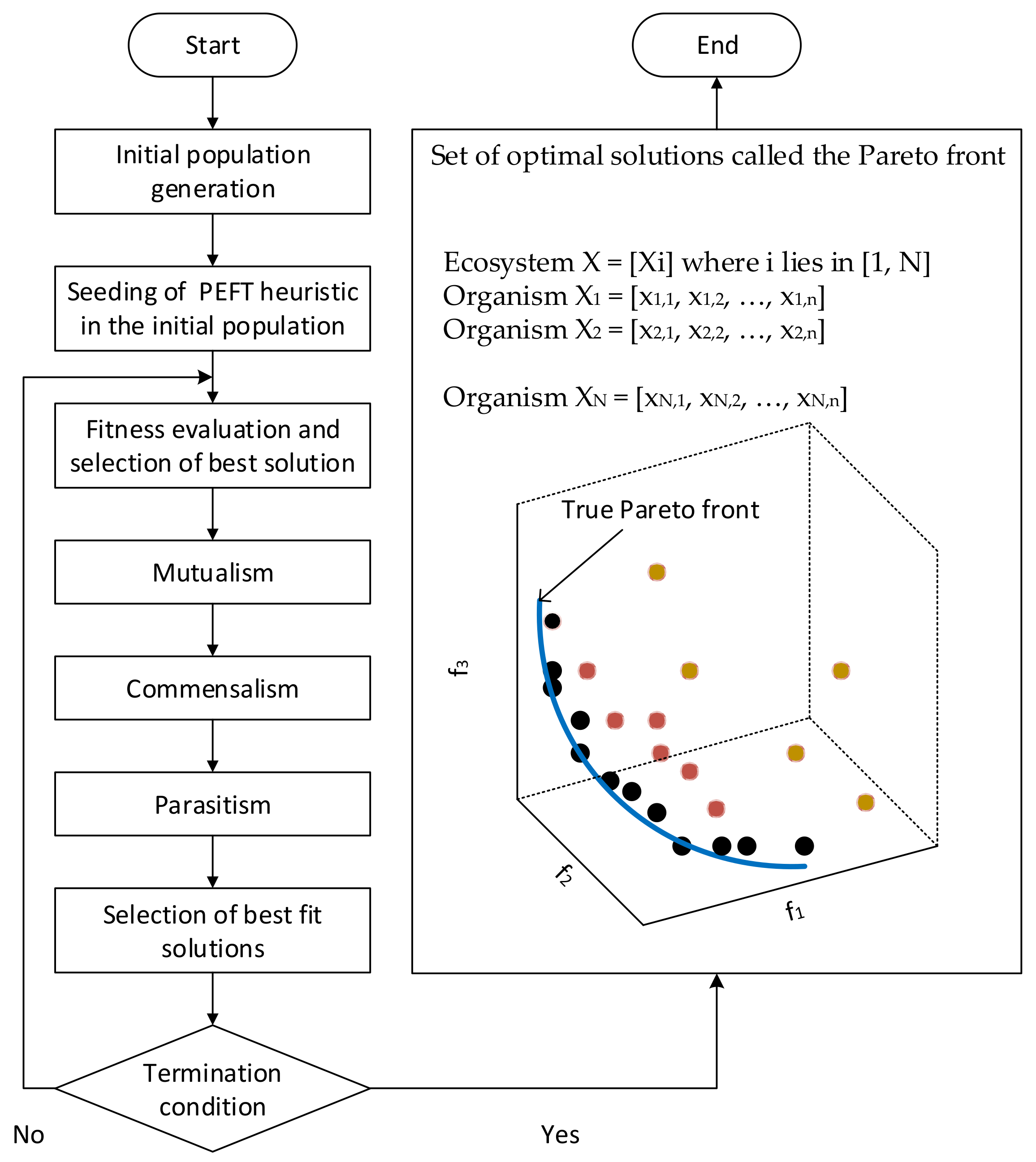
This section describes the proposed multi-objective workflow method HBMMO, which optimizes the scheduling of workflow tasks in the cloud environment. In this section, we show how we extended the discrete version of SOS in order to achieve the required objectives of minimizing both the makespan and the cost of executing workflows on the cloud and efficiently balance the load of the VMs. The flow diagram of the proposed algorithm is shown in Figure 2 and the pseudo code of our proposed HBMMO technique is presented in Algorithm 1. The following subsections represent the phases of the proposed algorithm.
4.1. Initialization
The first task of the proposed optimization model is generating a population of solution candidates, called an ecosystem, using different initialization schemes, where each candidate solution is called an organism. These organisms of the initial population include a schedule generated by the PEFT heuristic, and the remaining schedules are randomly generated under the condition that each organism satisfies all dependencies. The organisms generated by the PEFT heuristic could be used as an approximate endpoint of the Pareto front. The user is required to provide all the necessary inputs, including the size of the ecosystem, the number of VMs, and the number of objective functions. The PEFT heuristic provides guidance to the algorithm that improves the performance of the proposed method and allows for faster convergence to suboptimal solutions. By utilizing the PEFT heuristic, better initial candidate solutions may be obtained. The organisms adjust their position in the solution space through the three phases of the SOS algorithm. Each organism of the ecosystem represents a valid feasible schedule of the entire workflow and an organism’s length equals the size of the given workflow. Let be the number of organisms, be the number of tasks in a given workflow, and be the number of VMs for executing the workflow tasks, then the ecosystem is expressed as . The position of the organism, expressed as a vector of the element, can be given as
where such that . In other words, represents a task-VM mapping scheme of the workflow while preserving the precedence constraints. Table 2 shows an example of an organism for mapping of 10 tasks on 4 VMs. The best position identified by all organisms so far is represented by . Each organism of the ecosystem represents a mapping of the tasks of a given workflow to the VMs while keeping the precedence constraints. So, each organism represents a potential solution to the problem at hand in the solution space for the submitted workflow and the proposed algorithm is used to find the optimal solution.
4.2. Fitness Evaluation
At each iteration of the algorithm, the relationship among organisms (i.e., solutions) is decided based on the desired optimization fitness function using their corresponding positions according to Equation (3). Then, the organism with the best fitness value is updated.
4.3. Optimization
The optimization strategy is performed by applying the three search and update phases (i.e., mutualism, commensalism, and parasitism) to represent the symbiotic interaction between the organisms. The non-dominated organisms found along these phases are stored in an elite ecosystem. The three phases of the symbiotic relationships are described as follows.
4.3.1. Mutualism
The mutualism between organism and a randomly selected organism with is modeled in Equations (19)–(20).
where is known as the ‘Mutual Vector’, which represents the mutualistic characteristics between organism and to increase their survival advantage, R is a vector of uniformly distributed random numbers between 0 and 1, denotes the organism with the best objective fitness value in terms of the maximum level of adaptation in the ecosystem, and and are the adaptive benefit factors to represent the level of benefit to each of the two organisms and , respectively, which varies automatically during the search process. The adaptive benefit factors in [39] are shown as, ; ; and . The organisms are updated only if their new fitness is better than their pre-interaction fitness. Otherwise, and are discarded while and survive to the next population generation.
After mutualism, the elite ecosystem is shown in Equation (21).
4.3.2. Commensalism
The commensalism between organisms and with is modeled in Equation (22).
where is a vector of uniformly distributed random numbers between −1 and 1, and denotes the benefit given to by . The organism is updated by only if its new fitness is better than its pre-interaction fitness. Otherwise, is discarded while survives to the next population generation. After commensalism, the elite ecosystem is shown in Equation (23).
4.3.3. Parasitism
The parasitism between organism and a randomly selected organism with is implemented as follows.
Let be given a role similar to the anopheles mosquito through the creation of an artificial parasite termed as a Parasite Vector () in the search space by fine-tuning the stochastically selected attributes of organism in order to differentiate with . A random organism is selected as a host to and their fitness values are evaluated. If has better fitness value than , then is replaced by ; otherwise, will no longer be able to survive in the ecosystem. After parasitism, the elite ecosystem is shown in Equation (24).
4.4. Selection of Best Fit Solutions
The solutions from the elite ecosystem after the optimization process are combined together as given by Equation (25).
The size of the combined population is larger than the number of organisms in the ecosystem. The fitness of each organism in the ecosystem is checked for dominance with other members using Step IVB. Then, only organisms with higher ranks are selected based on fast non-dominated sorting and crowding distance [40] for the next generation. The solutions are selected based on the non-domination ranks in the front to which they belong. If there are more solutions with the same value of dominance, then the solution whose crowding distance is higher is selected for the next generation. The solution with the higher crowding distance value is less crowded by other solutions and signifies better density to preserve the diversity of the region. Each objective function is normalized prior to computing the crowding distance. Note that the size of the ecosystem comprising the best solutions is kept the same, that is . The solution with the highest rank is selected as the best solution for the next generation.
In the proposed work, the fitness evaluation function is normalized for converting all of the objectives into the minimized problems in the range [0, 1] and for maximizing the spread of the solutions across the Pareto front. The normalized fitness function value across objective functions of the solution is defined as
where is the th objective function value for solution , and and are the minimum and maximum values of the th objective function in the ecosystem.
The crowding distance is used to select the solutions who have the same rank in the front. The crowding distance of the two boundary solutions is assigned an infinite value. The crowding distance of an intermediate th solution in a non-dominated solution set is defined as the average distance of the two adjacent solutions on its either side along each of the objectives, denoted as , which is mathematically given in Equation (27).
where is the number of non-dominated solutions obtained, is an objective function value of a solution in the non-dominated set , is the th objective function value of the th solution in the set ; and the metrics and are the maximum and minimum normalized values of the th objective function in the same set, respectively. Here, the non-dominated solutions with the smallest and the largest objective function values, referred to as boundary solutions, are assigned an infinite distance value so that they are always selected.
4.5. Termination Condition
The termination condition is an important factor that can determine the final solutions from the simulation. In this study, the algorithm terminates when a maximum iterations criterion is satisfied. When the optimization process ends, the final set of all optimal solutions in the objective space, called the Pareto front, is presented to the user. According to the scenario presented in this study, a candidate solution is Pareto front if either it is at least as good as all other solutions for all the three objectives , , and , or it is better than all other solutions for at least one of these objectives.
| Algorithm 1. Hybrid Bio-inspired Metaheuristic for Multi-objective Optimization (HBMMO) for Scientific Workflow Scheduling in the Cloud. | |
| Input: | Workflow and set of VMs |
| Output: | Pareto optimal set of solutions |
| 1 | //Initialization phase (Section 4.1) |
| 2 | Initialize parameters |
| 3 | Initialize population with randomly generated solutions where each solution satisfies all constraints |
| 4 | Replace one of the organism by mapping generated by PEFT algorithm |
| 5 | Initialize |
| 6 | while termination criteria not fulfilled do |
| 7 | //Fitness evaluation phase (Section 4.2) |
| 8 | Evaluate the fitness of each organism //according to Equation (3) |
| 9 | Select the best solution as |
| 10 | //Optimization phase (Section 4.3) |
| 11 | //Apply Mutualism (Section 4.3.1) |
| 12 | Randomly select where |
| 13 | Update organisms and //according to Equations (19)–(20) |
| 14 | //Commensalism (Section 4.3.2) |
| 15 | Update //according to Equation (22) |
| 16 | //Parasitism (Section 4.3.3) |
| 17 | Randomly select where |
| 18 | Create a parasite vector () |
| 19 | if fitness of is better than then |
| 20 | accept to replace |
| 21 | else reject and keep |
| 22 | end if |
| 23 | //Selection of best fit solution phase (Section 4.4) |
| 24 | Generate the combined population |
| 25 | Calculate normalized fitness values for each objective //according to Equation (26) |
| 26 | Apply the non-dominated sort to find the solutions in fronts , where is min s.t. |
| 27 | for each front do |
| 28 | for each objective function do |
| 29 | for each // size of |
| 30 | Evaluate crowding distance of //according to Equation (27) |
| 31 | Sort according to crowding distance in descending order |
| 32 | end for |
| 33 | Calculate total crowding distance value for every front |
| 34 | end for |
| 35 | end for |
| 36 | Store the best solution as Pareto set in each generation |
| 37 | end while |
5. Performance Evaluation
5.1. Experimental Setup
The proposed HBMMO was implemented by conducting simulation experiments using an extension of CloudSim [41] called the WorkflowSim-1.0 toolkit [42], which is a modern framework aimed for modeling and simulating scientific workflow scheduling in cloud computing environments. It provides a higher layer of workflow management and also adds functionalities required to support the analysis of various scheduling overheads. Table 3 gives the parameters used in the simulation setup.
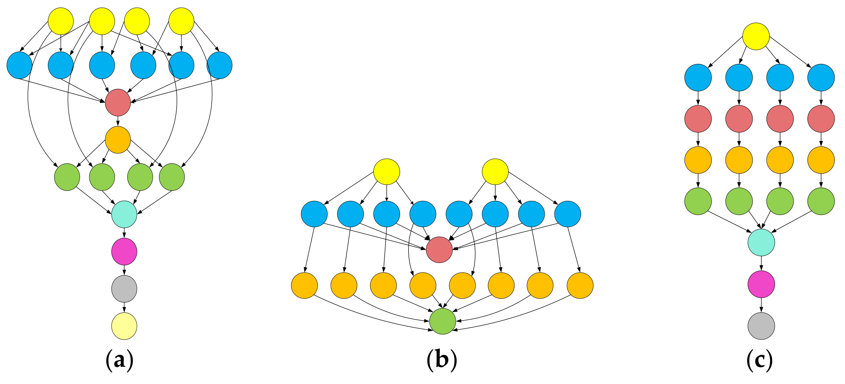
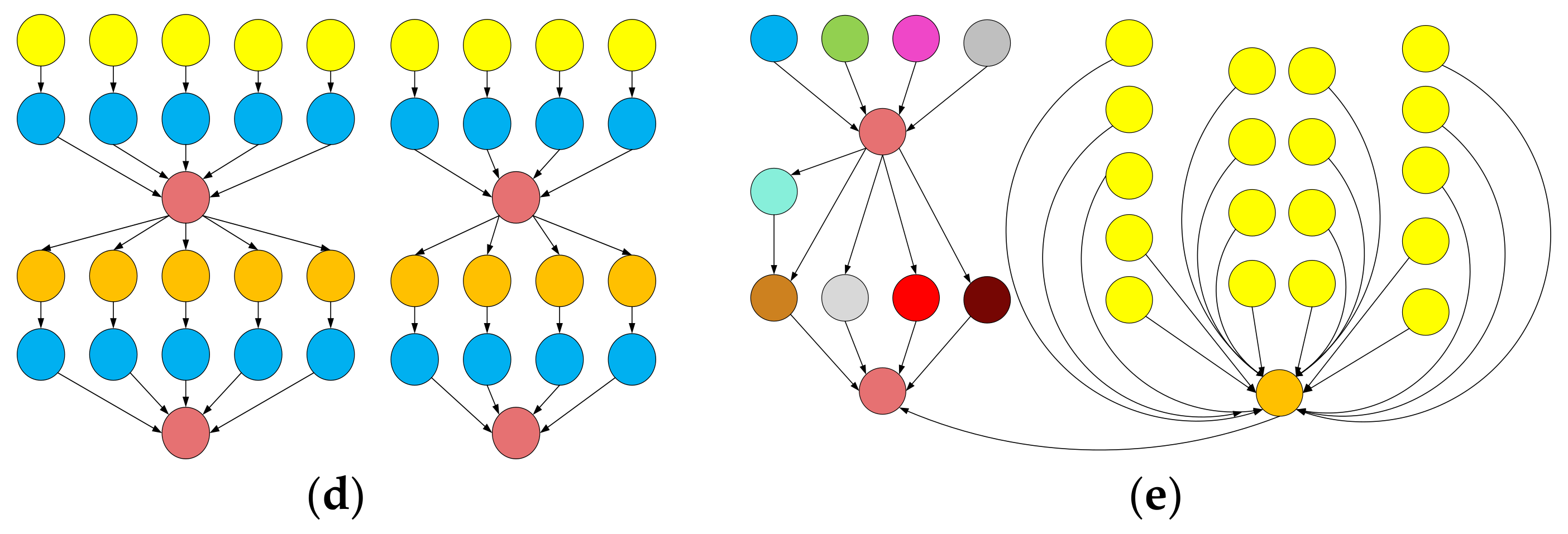
Experimentation was carried out with different real workflow applications published by Pegasus project, including Montage, CyberShake, Epigenomics, LIGO Inspiral Analysis, and SIPHT [43,44]. Montage is an input/output (I/O)-intensive astronomical application for constructing custom mosaics of the sky. CyberShake is a data-intensive application for generating probabilistic seismic hazard curves for a region. Epigenomics is a CPU-intensive workflow for automating various operations in genome sequence processing. LIGO Inspiral Analysis is a CPU-intensive workflow used for gravitational physics. SIPHT is a computation-intensive workflow used in bioinformatics for automating the search for untranslated RNA (sRNA) encoding-genes for bacterial replicons. Datasets of all the mentioned workflows are provided in the form of DAX files (https://confluence.pegasus.isi.edu/display/pegasus/WorkflowGenerator) in XML format. They are later converted to DAG-based workflows by using workflow management system framework tools, such as Pegasus [44]. Figure 3 shows the simplified representations of small instances of workflows used in our experiments and the characteristics of these workflows are presented in Table 4.
5.2. Evaluation Metrics
The performance analysis of the proposed algorithm is carried out with existing state-of-the-art algorithms using the following metrics.
5.2.1. Inverted Generational Distance ()
The inverted generational distance evaluates the proximity between the optimal solutions obtained by the proposed algorithm (that is, the obtained Pareto front) and the true Pareto front [40]. is mathematically given by [40] in Equation (28).
where is the number of non-dominated solutions obtained in the objective space along the Pareto front, and is the Euclidean distance (in objective space) between each solution and the nearest member of the true Pareto front. A result of indicates that all the optimal solutions generated by the proposed algorithm are in the true Pareto front; any other result represents its deviation from the true Pareto front. Therefore, a smaller value of generational distance (GD) reveals a better performance of the achieved solution set. In other words, closer proximity between the obtained Pareto front and the true Pareto front signifies better solutions.
5.2.2. Hypervolume ()
This metric indicates the volume of the objective space covered between the obtained Pareto front and a reference point [45]. For calculating hypervolume, first a vector of non-dominated solutions is generated as an approximation of the actual Pareto front, while the solutions dominated by this vector are discarded. A hypercube is created for each non-dominated solution obtained by the algorithms. Then, a union of all hypercubes is taken. is mathematically given in Equation (29).
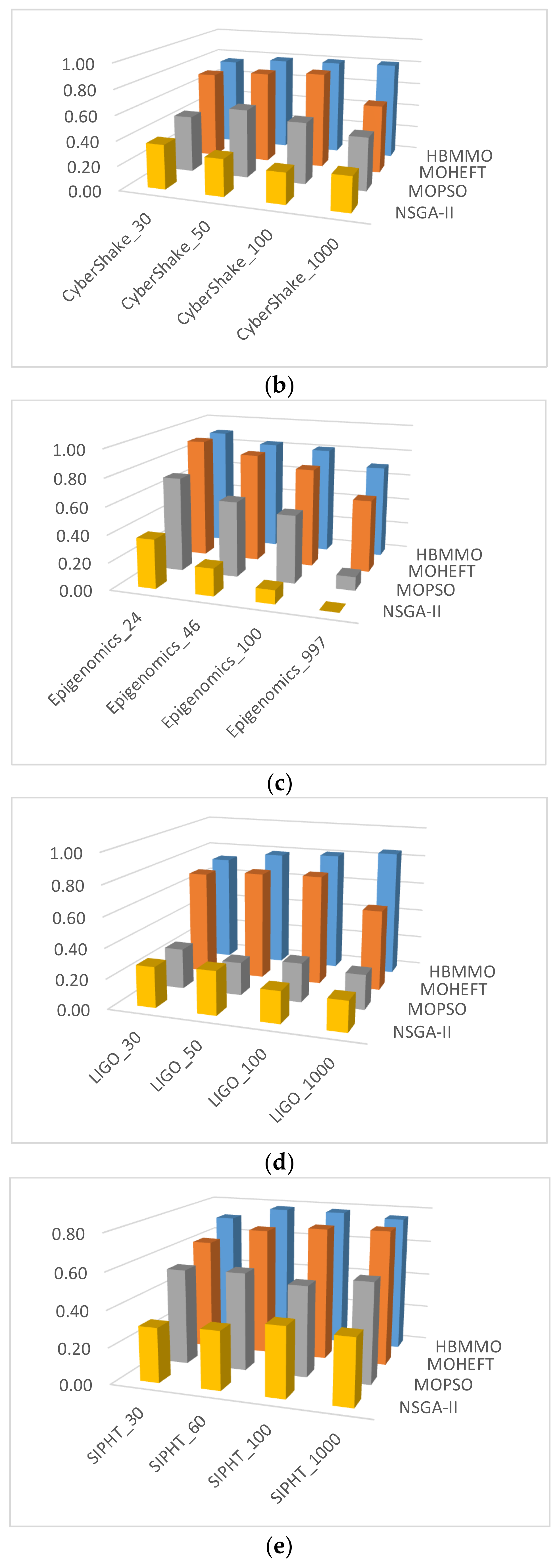
where is the hypercube for each solution . This metric is useful for providing combined information about the convergence and diversity of the Pareto optimal solutions. Algorithms that result in solutions with a large value of are desirable, because a larger value signifies that the solution set is close to the Pareto front and also has a good distribution. A result of indicates that there is no solution close to the true Pareto front and the corresponding algorithm fails to produce the optimal solution set. For the purpose of comparison between algorithms, the objective values of the obtained solutions are separately normalized between the interval [0, 1], with 1 representing the optimal value, before calculating the . In this study, a reference point (1, 1, 1) is selected in the calculations of .
5.3. Simaulation Results
The proposed HBMMO algorithm was evaluated against a set of well-known techniques to solve multi-objective optimization problem, including NSGA-II [40], MOPSO [46], and MOHEFT [3]. For the purpose of comparison, all algorithms employed the same number of evaluation functions. The parametric values for NSGA-II are set as: population size , maximum iterations , crossover rate , and mutation rate ; for MOPSO: population size , learning factors and , and inertia weight ; and for MOHEFT: number of trade-off solutions . To achieve the Pareto optimal solutions with the algorithms, the scheduling is repeated 50 times for each algorithm. The results are obtained by taking the average. The VMs are selected randomly such that the fastest VM is three times faster than the slowest one as well as three times more expensive.
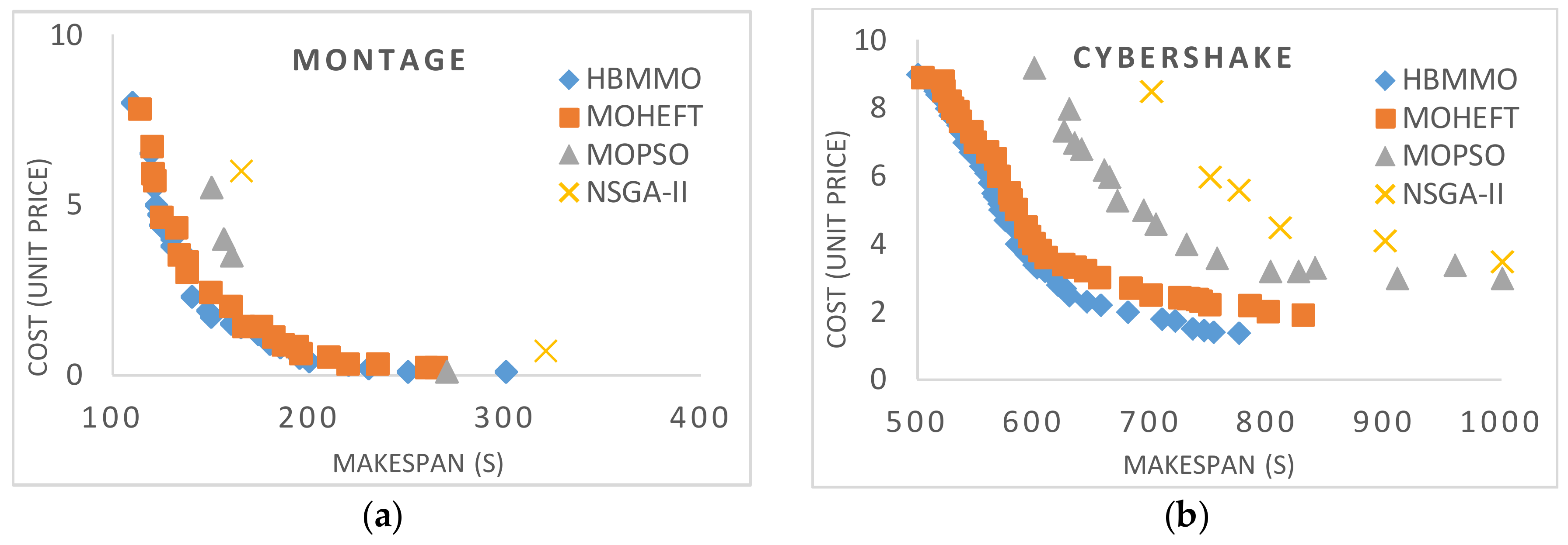
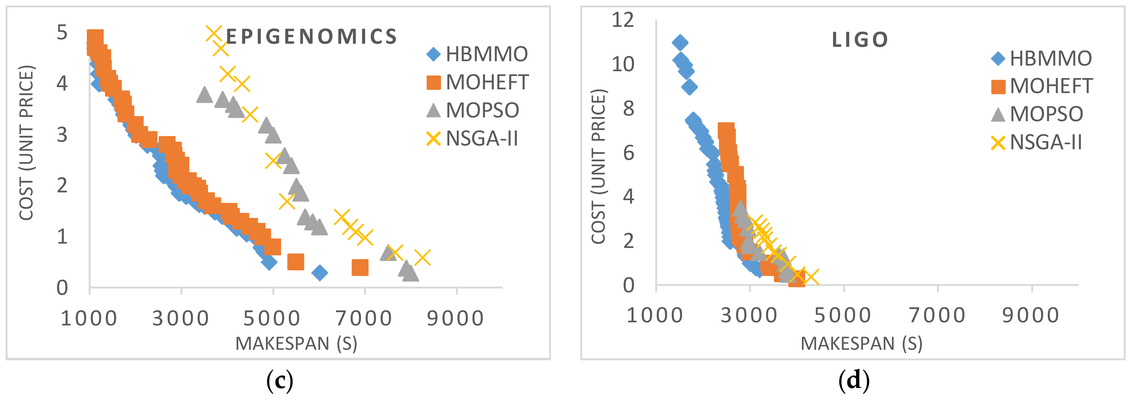
Figure 4 shows the multi-objective non-dominated solutions obtained for Montage, CyberShake, Epigenomics, and LIGO workflows, respectively. It shows that a lower makespan is correlated with a higher cost and vice versa. We can see that the solutions obtained using HBMMO have a better search ability due to the uniform distribution of solutions than those of MOHEFT, MOPSO, and NSGA-II. It can be seen that the Pareto fronts obtained using HBMMO are superior for all of the workflow instances under consideration. Even in the case of CyberShake, where MOHEFT performs significantly better, HBMMO is still able to maintain better convergence and a uniform distribution of solutions.
Figure 5 shows the results obtained by computing the mean GD for Montage with 25 tasks, CyberShake with 30 tasks, Epigenomics with 24 tasks, LIGO Inspiral Analysis with 30 tasks, and SIPHT with 30 tasks. It is observed that the GD value for the proposed HBMMO algorithm is lower as compared to other algorithms. It implies that the solution set generated by the proposed method has a better ability to converge towards the true Pareto front.
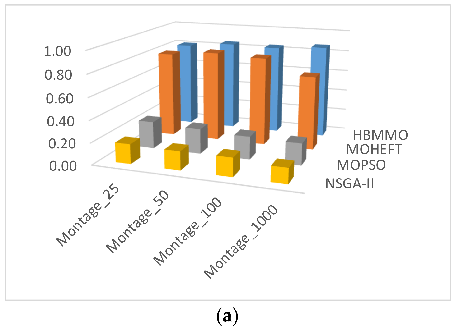
As can be seen from Figure 6, the mean of the HBMMO against the comparative algorithms is statistically better in most of the scenarios. Compared with NSGA-II, the performance gain is over 50% in most of the cases whereas the improvement rate of HBMMO over MOHEFT is slightly better for small- and medium-size workflows. It can be concluded that HBMMO has better search efficiency and can achieve better non-dominated fronts.
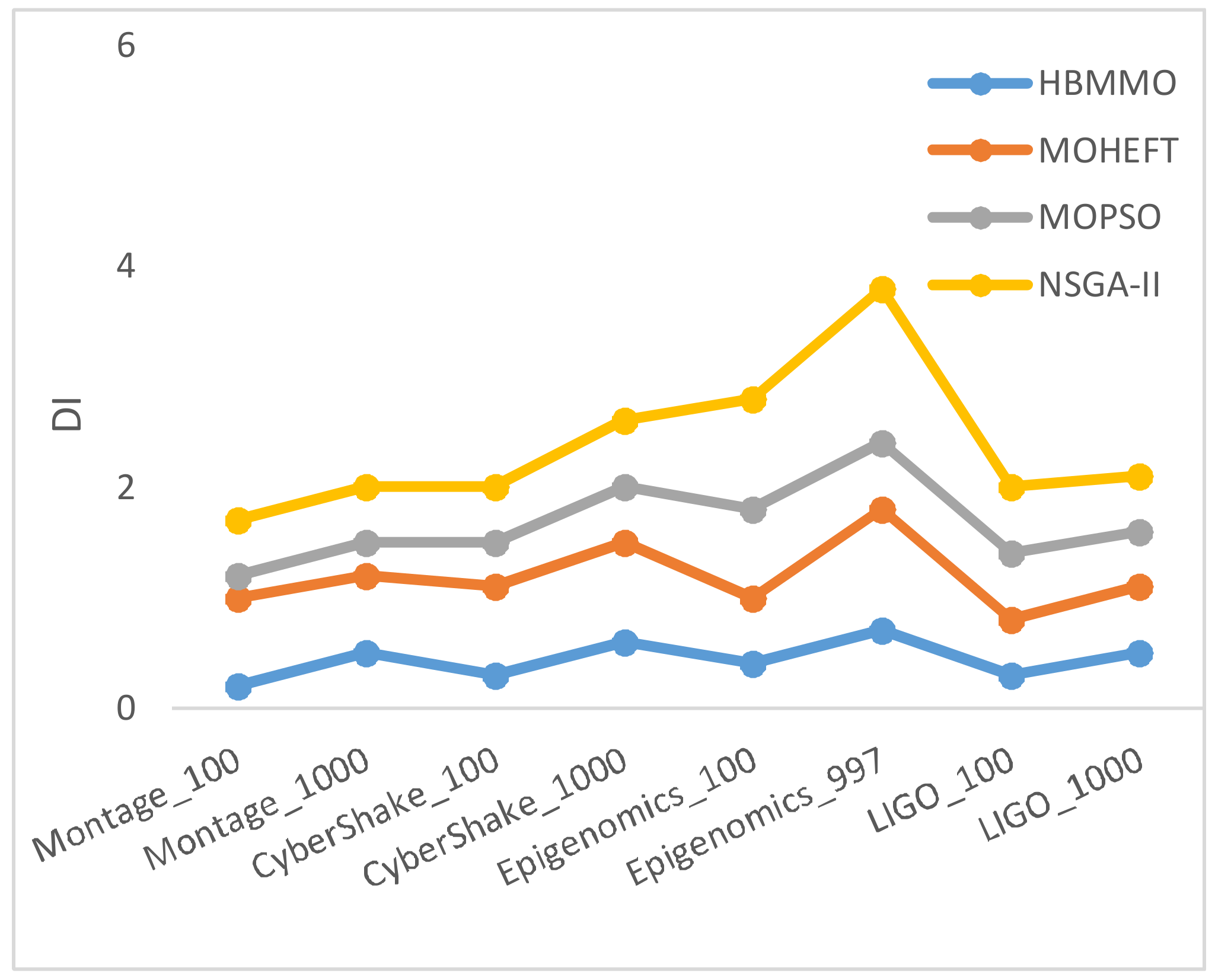
Figure 7 shows a graph of the average Degree of Imbalance () of tasks among VMs. It describes the fairness of the tasks’ distribution across the VMs. HBMMO has the best load distribution of tasks between the VMs. Therefore, the smaller value of DI reveals the better performance of the achieved solution set.
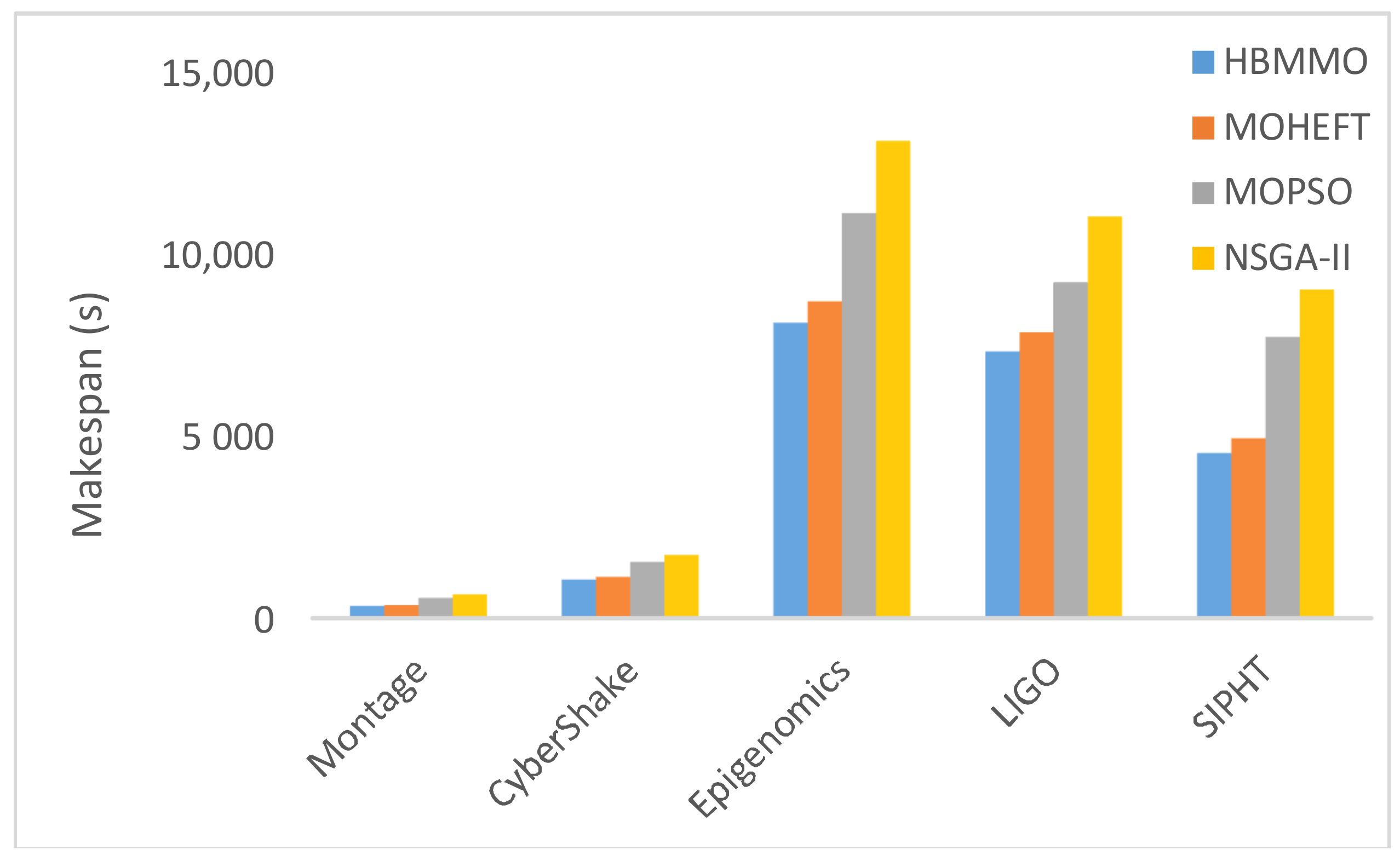
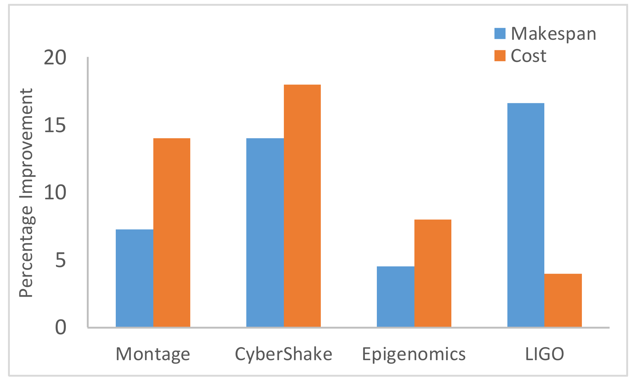
Figure 8 shows that HBMMO achieves a better average makespan than the comparative algorithms for all of the benchmark workflows. Figure 9 shows the improvement rate of HBMMO over the MOHEFT algorithm in terms of makespan and cost of the workflow applications. In the case of makespan, the HBMMO gains an improvement by 7.26%, 14.04%, 4.54%, and 16.6% compared with the MOHEFT, using the Montage, CyberShake, Epigenomics, and LIGO workflows, respectively. The cost of HBMMO was better by 14%, 18%, 8%, and 4% over the MOHEFT algorithm in the case of the Montage, CyberShake, Epigenomics, and LIGO workflows, respectively.
5.4. Analysis of Variance (ANOVA) Test
The statistical significance of the achieved experimental results is validated by applying the one-way ANOVA test [47]. It is used to find out whether there is any significance variation in the means of all groups or not. It includes a null hypothesis and an alternate hypothesis given as
where states that there is no significant difference between the results of the groups and states that there is significant difference between the results of the groups.
Table 5 shows the results for each workflow. It can be seen that the difference between the groups is significant whereas the difference within the groups is trivial. It is clear that the proposed method is statistically significant from the comparative algorithm due to the greater F-statistic and lower p-value. The p-values in the tests are extremely small or close to zero, so they are not given here. Thus, the null hypothesis is rejected and the alternate hypothesis is accepted. Therefore, it is evident that the proposed HBMMO significantly outperforms the other state-of-the-art algorithms.
6. Conclusions and Future Work
In this paper, a novel Hybrid Bio-inspired Metaheuristic for Multi-objective Optimization (HBMMO) algorithm based on a non-dominant sorting strategy for the workflow scheduling problem in the cloud with more than two objectives is proposed and implemented using WorkflowSim. It is a hybridization of the list-based heuristic algorithm PEFT and the discrete version of the metaheuristic algorithm SOS, which aims to minimize the overall makespan, overall execution cost, and inefficient utilization of the VMs. Well-known real-world workflows are selected to evaluate the performance of the proposed method and the results demonstrate that the proposed HBMMO algorithm is highly effective and promising with potentially wide applicability for the scientific workflow scheduling problem in an IaaS cloud, and attains a uniformly distributed solution set with better convergence towards the true Pareto optimal front. In future work, we intend to develop an environment friendly distributed scheduler for VMs between cloud data centers so that energy can be saved and CO2 emissions can be reduced.
Author Contributions
Nazia Anwar carried out the conception and design of the study, performed the experiments, analyzed and interpreted the data, and contributed to drafting and revising the manuscript. Huifang Deng made substantial contributions to the design of the study and the analysis and interpretation of the data and critically reviewed the manuscript. All authors read and approved the final manuscript.
Conflicts of Interest
The authors declare no conflict of interest.
References
- Ostrowski, K.; Birman, K.; Doley, D. Extensible architecture for high-performance, scalable, reliable publish-subscribe eventing and notification. Int. J. Web Serv. Res. 2007, 4, 18–58. [Google Scholar] [CrossRef]
- Zhu, Z.M.; Zhang, G.X.; Li, M.Q.; Liu, X.H. Evolutionary multi-objective workflow scheduling in cloud. IEEE Trans. Parallel Distrib. Syst. 2016, 27, 1344–1357. [Google Scholar] [CrossRef]
- Durillo, J.J.; Prodan, R. Multi-objective workflow scheduling in Amazon EC2. Clust. Comput. 2014, 17, 169–189. [Google Scholar] [CrossRef]
- Coello, C.A.C. Evolutionary multi-objective optimization: A historical view of the field. IEEE Comput. Intell. Mag. 2006, 1, 28–36. [Google Scholar] [CrossRef]
- Arabnejad, H.; Barbosa, J.G. List scheduling algorithm for heterogeneous systems by an optimistic cost table. IEEE Comput. Intell. Mag. 2014, 25, 682–694. [Google Scholar] [CrossRef]
- Choudhary, A.; Gupta, I.; Singh, V.; Jana, P.K. A GSA based hybrid algorithm for bi-objective workflow scheduling in cloud computing. Future Gener. Comput. Syst. 2018. [Google Scholar] [CrossRef]
- Fard, H.M.; Prodan, R.; Fahringer, T. Multi-objective list scheduling of workflow applications in distributed computing infrastructures. J. Parallel Distrib. Comput. 2014, 74, 2152–2165. [Google Scholar] [CrossRef]
- Cheng, M.Y.; Prayogo, D. Symbiotic Organisms Search: A new metaheuristic optimization algorithm. Comput. Struct. 2014, 139, 98–112. [Google Scholar] [CrossRef]
- Abdullahi, M.; Ngadi, M.A.; Abdulhamid, S.M. Symbiotic Organism Search optimization based task scheduling in cloud computing environment. Future Gener. Comput. Syst. 2016, 56, 640–650. [Google Scholar] [CrossRef]
- Topcuoglu, H.; Hariri, S.; Wu, M.Y. Performance-effective and low-complexity task scheduling for heterogeneous computing. IEEE Trans. Parall. Distrib. Syst. 2002, 13, 260–274. [Google Scholar] [CrossRef]
- Beloglazov, A.; Abawajy, J.; Buyya, R. Energy-aware resource allocation heuristics for efficient management of data centers for cloud computing. Future Gener. Comput. Syst. 2012, 28, 755–768. [Google Scholar] [CrossRef]
- Frincu, M.E. Scheduling highly available applications on cloud environments. Future Gener. Comput. Syst. 2014, 32, 138–153. [Google Scholar] [CrossRef]
- Yao, G.S.; Ding, Y.S.; Jin, Y.C.; Hao, K.R. Endocrine-based coevolutionary multi-swarm for multi-objective workflow scheduling in a cloud system. Soft Comput. 2017, 21, 4309–4322. [Google Scholar] [CrossRef]
- Nasonov, D.; Visheratin, A.; Butakov, N.; Shindyapina, N.; Melnik, M.; Boukhanovsky, A. Hybrid evolutionary workflow scheduling algorithm for dynamic heterogeneous distributed computational environment. J. Appl. Logic 2017, 24, 50–61. [Google Scholar] [CrossRef]
- Anwar, N.; Deng, H. Elastic scheduling of scientific workflows under deadline constraints in cloud computing environments. Future Internet 2018, 10, 5. [Google Scholar] [CrossRef]
- Madni, S.H.H.; Latiff, M.S.A.; Coulibaly, Y.; Abdulhamid, S.M. An appraisal of meta-heuristic resource allocation techniques for IaaS cloud. Indian J. Sci. Technol. 2016, 9. [Google Scholar] [CrossRef]
- Singh, P.; Dutta, M.; Aggarwal, N. A review of task scheduling based on meta-heuristics approach in cloud computing. Knowl. Inf. Syst. 2017, 52, 1–51. [Google Scholar] [CrossRef]
- Domanal, S.; Guddeti, R.M.; Buyya, R. A hybrid bio-inspired algorithm for scheduling and resource management in cloud environment. IEEE Serv. Comput. 2017, PP, 99. [Google Scholar] [CrossRef]
- Pooranian, Z.; Shojafar, M.; Abawajy, J.H.; Abraham, A. An efficient meta-heuristic algorithm for grid computing. J. Comb. Optim. 2015, 30, 413–434. [Google Scholar] [CrossRef]
- Abdullahi, M.; Ngadi, M.A. Hybrid symbiotic organisms search optimization algorithm for scheduling of tasks on cloud computing environment. PLoS ONE 2016, 11, e0158229. [Google Scholar] [CrossRef]
- Zhang, F.; Cao, J.W.; Li, K.Q.; Khan, S.U.; Hwang, K. Multi-objective scheduling of many tasks in cloud platforms. Future Gener. Comput. Syst. 2014, 37, 309–320. [Google Scholar] [CrossRef]
- Su, S.; Li, J.; Huang, Q.J.; Huang, X.; Shuang, K.; Wang, J. Cost-efficient task scheduling for executing large programs in the cloud. Parallel Comput. 2013, 39, 177–188. [Google Scholar] [CrossRef]
- Xu, H.; Yang, B.; Qi, W.; Ahene, E. A multi-objective optimization approach to workflow scheduling in clouds considering fault recovery. KSII Trans. Internet Inf. Syst. 2016, 10. [Google Scholar] [CrossRef]
- Casas, I.; Taheri, J.; Ranjan, R.; Wang, L.Z.; Zomaya, A.Y. A balanced scheduler with data reuse and replication for scientific workflows in cloud computing systems. Future Gener. Comput. Syst. 2016, 74, 168–178. [Google Scholar] [CrossRef]
- Hu, H.Z.; Tian, S.L.; Guo, Q.; Ouyang, A.J. An adaptive hybrid PSO multi-objective optimization algorithm for constrained optimization problems. Int. J. Pattern Recognit. Artif. Intell. 2015, 29, 1559009. [Google Scholar] [CrossRef]
- Ouyang, A.J.; Li, K.L.; Fei, X.W.; Zhou, X.; Duan, M.X. A novel hybrid multi-objective population migration algorithm. Int. J. Pattern Recognit. Artif. Intell. 2015, 29, 1559001. [Google Scholar] [CrossRef]
- Panda, A.; Pani, S. A Symbiotic Organisms Search algorithm with adaptive penalty function to solve multi-objective constrained optimization problems. Appl. Soft Comput. 2016, 46, 344–360. [Google Scholar] [CrossRef]
- Verma, A.; Kaushal, S. A hybrid multi-objective Particle Swarm Optimization for scientific workflow scheduling. Parallel Comput. 2017, 62, 1–19. [Google Scholar] [CrossRef]
- Ye, X.; Li, J.; Liu, S.; Liang, J.; Jin, Y. A hybrid instance-intensive workflow scheduling method in private cloud environment. Nat. Comput. 2017, 1–12. [Google Scholar] [CrossRef]
- Goulart, F.; Campelo, F. Preference-guided evolutionary algorithms for many-objective optimization. Inf. Sci. 2016, 329, 236–255. [Google Scholar] [CrossRef]
- Zhu, Z.X.; Xiao, J.; He, S.; Ji, Z.; Sun, Y.W. A multi-objective memetic algorithm based on locality-sensitive hashing for one-to-many-to-one dynamic pickup-and-delivery problem. Inf. Sci. 2016, 329, 73–89. [Google Scholar] [CrossRef]
- Deb, K.; Jain, H. An evolutionary many-objective optimization algorithm using reference-point-based non-dominated sorting approach, Part I: Solving problems with box constraints. IEEE Trans. Evol. Comput. 2014, 18, 577–601. [Google Scholar] [CrossRef]
- Ostermann, S.; Iosup, A.; Yigibasi, N.; Prodan, R.; Fahringer, T.; Epema, D. A performance analysis of EC2 cloud computing services for scientific computing. In Cloud Computing. CloudComp 2009; Lecture Notes of the Institute for Computer Sciences, Social-Informatics and Telecommunications Engineering; Springer: Berlin/Heidelberg, Germany, 2010; Volume 34. [Google Scholar] [CrossRef]
- Mao, M.; Humphrey, M. Auto-scaling to minimize cost and meet application deadlines in cloud workflows. In Proceedings of the International Conference for High Performance Computing, Networking, Storage and Analysis, Seatle, WA, USA, 12–18 November 2011. [Google Scholar] [CrossRef]
- Singh, V.; Gupta, I.; Jana, P.K. A novel cost-efficient approach for deadline-constrained workflow scheduling by dynamic provisioning of resources. Future Gener. Comput. Syst. 2018, 79, 95–110. [Google Scholar] [CrossRef]
- Rodriguez, M.A.; Buyya, R. Budget-driven scheduling of scientific workflows in IaaS clouds with fine-grained billing periods. ACM Trans. Auton. Adapt. Syst. 2017, 12, 5. [Google Scholar] [CrossRef]
- Schad, J.; Dittrich, J.; Quiane-Ruiz, J.A. Runtime measurements in the cloud: Observing, analyzing, and reducing variance. Proc. VLDB Endow. 2010, 3, 460–471. [Google Scholar] [CrossRef]
- Schad, J. Understanding and Managing the Performance Variation and Data Growth in Cloud Computing. Doctoral Thesis, Saarland University, Saarbruken, Germany, May 2015. [Google Scholar]
- Ezugwu, A.E.; Adewumi, A.O. Soft sets based symbiotic organisms search algorithm for resource discovery in cloud computing environment. Future Gener. Comput. Syst. 2017, 76, 33–55. [Google Scholar] [CrossRef]
- Deb, K.; Pratap, A.; Agarwal, S.; Meyarivan, T. A fast and elitist multiobjective genetic algorithm: NSGA-II. IEEE Trans. Evol. Comput. 2002, 6, 182–197. [Google Scholar] [CrossRef]
- Calheiros, R.N.; Ranjan, R.; Beloglazov, A.; de Rose, C.A.F.; Buyya, R. CloudSim: A toolkit for modeling and simulation of cloud computing environments and evaluation of resource provisioning algorithms. Softw. Pract. Exp. 2011, 41, 23–50. [Google Scholar] [CrossRef]
- Chen, W.; Deelman, E. WorkflowSim: A toolkit for simulating scientific workflows in distributed environments. In Proceedings of the 2012 IEEE 8th International Conference on E-Science (e-Science), Chicago, IL, USA, 8–12 October 2012; pp. 1–12. [Google Scholar] [CrossRef]
- Juve, G.; Chervenak, A.; Deelman, E.; Bharathi, S.; Mehta, G.; Vahi, K. Characterizing and profiling scientific workflows. Future Gener. Comput. Syst. 2013, 29, 682–692. [Google Scholar] [CrossRef]
- Deelman, E.; Vahi, K.; Juve, G.; Rynge, M.; Callaghan, S.; Maechling, P.J.; Mayani, R.; Chen, W.; da Silva, R.F.; Livny, M.; et al. Pegasus, a workflow management system for science automation. Future Gener. Comput. Syst. 2015, 46, 17–35. [Google Scholar] [CrossRef]
- Zitzler, E.; Thiele, L.; Laumanns, M.; Fonseca, C.M.; da Fonseca, V.G. Performance assessment of multiobjective optimizers: An analysis and review. IEEE Trans. Evol. Comput. 2003, 7, 117–132. [Google Scholar] [CrossRef]
- Coello, C.A.C.; Pulido, G.T.; Lechuga, M.S. Handling multiple objectives with Particle Swarm Optimization. IEEE Trans. Evol. Comput. 2004, 8, 256–279. [Google Scholar] [CrossRef]
- Muller, K.E.; Fetterman, B.A. Regression and ANOVA: An Integrated Approach Using SAS Software; SAS Institute: Cary, NC, USA, 2002. [Google Scholar]
Figure 1.
Block diagram of proposed workflow scheduling model.

Figure 2.
Flowchart of the proposed model. PEFT: Predict Earliest Finish Time.

Figure 3.
The structure of workflows used for: (a) Montage; (b) CyberShake; (c) Epigenomics; (d) LIGO Inspiral Analysis; (e) SIPHT.
Figure 3.
The structure of workflows used for: (a) Montage; (b) CyberShake; (c) Epigenomics; (d) LIGO Inspiral Analysis; (e) SIPHT.


Figure 4.
Bi-objective Pareto fronts for benchmark workflows: (a) Montage_25; (b) CyberShake_30; (c) Epigenomics_24; (d) LIGO_30.
Figure 4.
Bi-objective Pareto fronts for benchmark workflows: (a) Montage_25; (b) CyberShake_30; (c) Epigenomics_24; (d) LIGO_30.


Figure 5.
Generational distance obtained after 15 runs of the benchmark workflows.
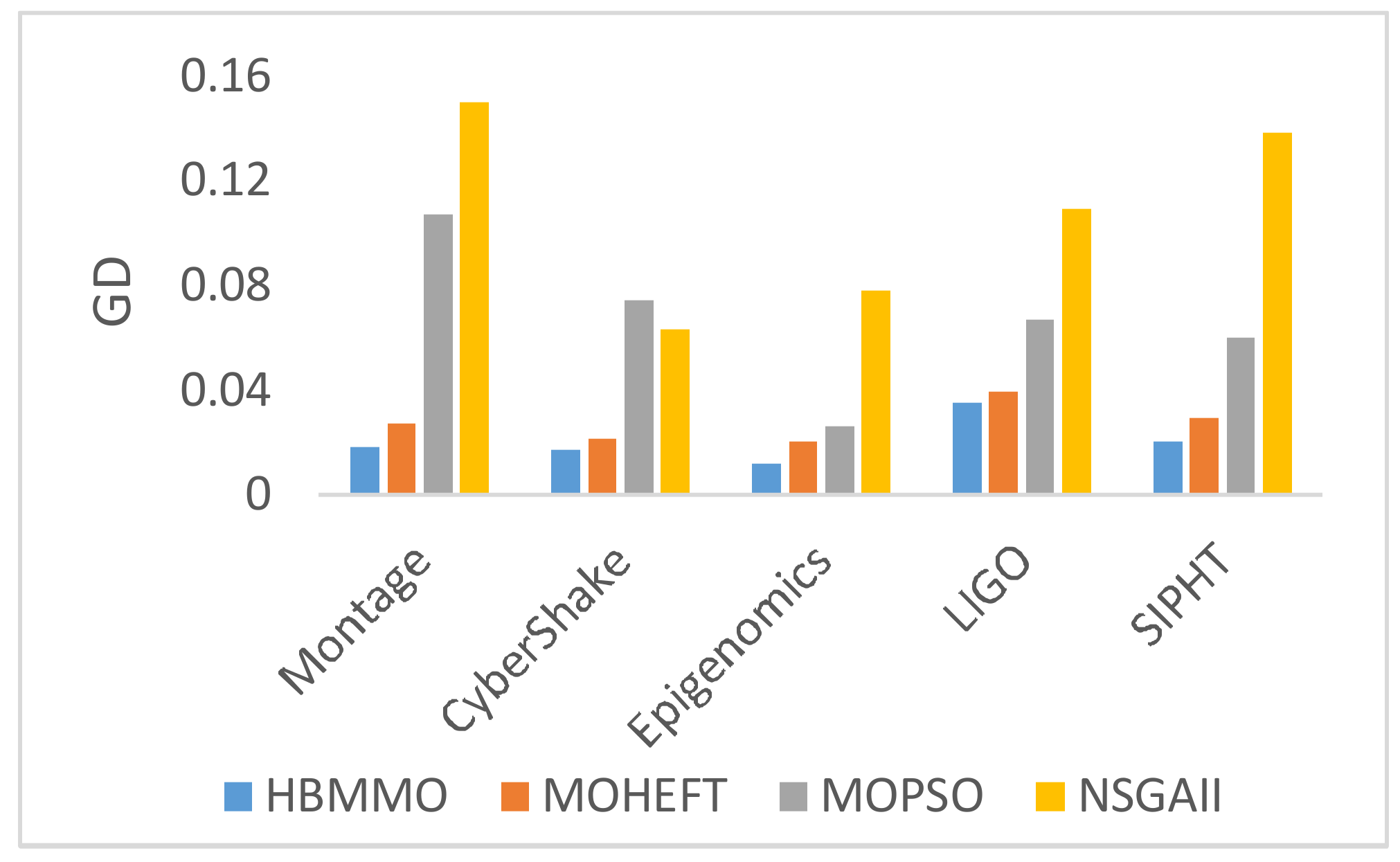
Figure 6.
Comparison of -metric for different algorithms on benchmark workflows: (a) Montage; (b) CyberShake; (c) Epigenomics; (d) LIGO; (e) SIPHT.
Figure 6.
Comparison of -metric for different algorithms on benchmark workflows: (a) Montage; (b) CyberShake; (c) Epigenomics; (d) LIGO; (e) SIPHT.


Figure 7.
Comparison of Degree of Imbalance () of tasks among VMs.

Figure 8.
Comparison of average makespan for different algorithms.

Figure 9.
Comparative analysis of makespan and cost of HBMMO versus MOHEFT on benchmark workflows.


Table 1.
Notations and their semantics.
| Notation | Description |
|---|---|
| Set of tasks of the workflow, represented by vertices of the Directed Acyclic Graph (DAG) | |
| Set of Virtual Machines (VMs) | |
| Number of tasks in a given workflow | |
| Number of available VMs | |
| th task, | |
| th VM, | |
| Entry task of the given workflow | |
| Exit task of the given workflow | |
| Predecessors (or parents set) of | |
| Successors (or children set) | |
| Ecosystem (i.e., population) size, or in other words, the number of organisms (i.e., candidate solutions) in the ecosystem | |
| An ecosystem representing several candidate solutions | |
| th organism of representing a candidate solution corresponding to allocation of the whole workflow tasks over the available VMs | |
| Best organism known so far | |
| An integer representing the VM allocated to the task such that | |
| Number of objective functions | |
| Fitness function, including | |
| Makespan | |
| Cost | |
| Degree of imbalance of VMs | |
| Normalized fitness evaluation function of the solution across the objectives | |
| Binary variable, if task is executed on VM , ; otherwise | |
| Workload (i.e., service length) of task measured by Millions of Instructions (MI) | |
| Central Processing Unit (CPU) computing capacity of VM measured by Millions of Instruction Per Second (MIPS) | |
| Data transfer size from task to | |
| Bandwidth of VM | |
| Start time of task executed on VM | |
| Execution time of task running on VM | |
| Communication time between task and ; if the tasks are executed on same VM, | |
| Finish time of task executed on VM | |
| Available time of VM for the execution of task | |
| Finish time of last task | |
| Cost per interval unit of VM type | |
| Billing interval of VM type | |
| Execution cost of task on VM | |
| Data transfer cost per time unit for VM | |
| VM performance variability | |
| Execution makespan of workflow | |
| Degree of imbalance among VMs | |
| Utilization rate of VM |
Table 2.
Example of an organism representing task-VM mapping.
| Task ID | |||||||||||
| VM ID | 1 | 3 | 2 | 2 | 4 | 1 | 3 | 1 | 3 | 4 | 2 |
Table 3.
Configuration details of simulation studies.
| Parameter | Value |
|---|---|
| Number of tasks | (20–1000) |
| Number of VMs | 8 |
| MIPS | 500–1500 |
| RAM | (512–2048) MB |
| Bandwidth | 1 MBps |
| Number of processors | 2 |
| Population size | 100 |
| Maximum iterations | 500 |
| Number of simulation runs | 50 |
Table 4.
Characteristics of the benchmark workflows.
| Workflow | Number of Nodes | Number of Edges | Mean Data Size (MB) |
|---|---|---|---|
| Montage_25 | 25 | 95 | 3.43 |
| Montage_50 | 50 | 206 | 3.36 |
| Montage_100 | 100 | 433 | 3.23 |
| Montage_1000 | 1000 | 4485 | 3.21 |
| CyberShake_30 | 30 | 112 | 747.48 |
| CyberShake_50 | 50 | 188 | 864.74 |
| CyberShake_100 | 100 | 380 | 849.60 |
| CyberShake_100 | 1000 | 3988 | 102.29 |
| Epigenomics_24 | 24 | 75 | 116.20 |
| Epigenomics_46 | 46 | 148 | 104.81 |
| Epigenomics_100 | 100 | 322 | 395.10 |
| Epigenomics_997 | 997 | 3228 | 388.59 |
| LIGO_30 | 30 | 95 | 9.00 |
| LIGO_50 | 50 | 160 | 9.16 |
| LIGO_100 | 100 | 319 | 8.93 |
| LIGO_1000 | 1000 | 3246 | 8.90 |
| SIPHT_30 | 30 | 91 | 7.73 |
| SIPHT_60 | 60 | 198 | 6.95 |
| SIPHT_100 | 100 | 335 | 6.27 |
| SIPHT_1000 | 1000 | 3528 | 5.91 |
Table 5.
One-way ANOVA test result.
| Workflow | Source of Variation | SS | df | MS | F |
|---|---|---|---|---|---|
| Montage_1000 | Between groups | 5.20 × 10⁻⁷ | 2 | 2.6 × 10⁻⁷ | 9.3 × 10³ |
| Within groups | 7.50 × 10⁻¹⁰ | 27 | 2.8 × 10⁻¹¹ | ||
| Total | 5.2 × 10⁻⁷ | 29 | |||
| CyberShake_1000 | Between groups | 2.9 × 10⁻¹² | 2 | 1.45 × 10⁻¹¹ | 2.3 × 10⁴ |
| Within groups | 1.7 × 10⁻¹⁴ | 27 | 6.3 × 10⁻¹⁶ | ||
| Total | 2.9 × 10⁻¹² | 29 | |||
| Epigenomics_997 | Between groups | 1.3 × 10⁻¹² | 2 | 6.5 × 10⁻¹³ | 1.5 × 10³ |
| Within groups | 1.2 × 10⁻¹⁴ | 27 | 4.4 × 10⁻¹⁶ | ||
| Total | 1.3 × 10⁻¹² | 29 | |||
| LIGO_1000 | Between groups | 6.5 × 10⁻¹¹ | 2 | 3.2 × 10⁻¹¹ | 1.8 × 10³ |
| Within groups | 4.9 × 10⁻¹³ | 27 | 1.8 × 10⁻¹⁴ | ||
| Total | 6.5 × 10⁻¹¹ | 29 | |||
| SIPHT_1000 | Between groups | 2.1 × 10⁻¹⁰ | 2 | 1.05 × 10⁻¹⁰ | 1.2 × 10³ |
| Within groups | 2.4 × 10⁻¹² | 27 | 8.9 × 10⁻¹⁴ | ||
| Total | 2.1 × 10⁻¹⁰ | 29 |
© 2018 by the authors. Licensee MDPI, Basel, Switzerland. This article is an open access article distributed under the terms and conditions of the Creative Commons Attribution (CC BY) license (http://creativecommons.org/licenses/by/4.0/).
Share and Cite
MDPI and ACS Style
Anwar, N.; Deng, H. A Hybrid Metaheuristic for Multi-Objective Scientific Workflow Scheduling in a Cloud Environment. Appl. Sci. 2018, 8, 538. https://doi.org/10.3390/app8040538
AMA Style
Anwar N, Deng H. A Hybrid Metaheuristic for Multi-Objective Scientific Workflow Scheduling in a Cloud Environment. Applied Sciences. 2018; 8(4):538. https://doi.org/10.3390/app8040538
Chicago/Turabian StyleAnwar, Nazia, and Huifang Deng. 2018. "A Hybrid Metaheuristic for Multi-Objective Scientific Workflow Scheduling in a Cloud Environment" Applied Sciences 8, no. 4: 538. https://doi.org/10.3390/app8040538
Note that from the first issue of 2016, this journal uses article numbers instead of page numbers. See further details here.