A Collaborative Multiplicative Holt-Winters Forecasting Approach with Dynamic Fuzzy-Level Component

Abstract

The adoption of forecasting approaches such as the multiplicative Holt-Winters (MHW) model is preferred in business, especially for the prediction of future events having seasonal and other causal variations. However, in the MHW model the initial values of the time-series parameters and smoothing constants are incorporated by a recursion process to estimate and update the level (L_T), growth rate (b_T) and seasonal component (SN_T). The current practice of integrating and/or determining the initial value of L_T is a stationary process, as it restricts the scope of adjustment with the progression of time and, thereby, the forecasting accuracy is compromised, while the periodic updating of L_T is avoided, presumably due to the computational complexity. To overcome this obstacle, a fuzzy logic-based prediction model is developed to evaluate L_T dynamically and to embed its value into the conventional MHW approach. The developed model is implemented in the MATLAB Fuzzy Logic Toolbox along with an optimal smoothing constant-seeking program. The new model, proposed as a collaborative approach, is tested with real-life data gathered from a local manufacturer and also for two industrial cases extracted from literature. In all cases, a significant improvement in forecasting accuracy is achieved.

1. Introduction

In the contemporary world of business, due to frequent technological advancements and operational changes, competition, complexities and challenges have increased drastically [1]. Moreover, easier access to international markets, expeditious technological advancement and the ceaseless requirements of quality products has complicated the scenarios for manufacturers. Hence, to contend with this dynamic but uncertain environment, manufacturers have no choice other than hastening their steps to gratify customers’ demands on time and efficiently [2]. In this regard, the urge for a more accurate and reliable forecasting approach cannot be overlooked.

Plenty of forecasting approaches with innovative ideas have been proposed in the recent past which are broadly classified as qualitative and quantitative techniques. In the qualitative approach, prediction is made on the basis of the market dissection and the judgement of the experienced managers, whereas, the quantitative techniques mainly focus on historical data. However, in the latter forecasting class, the decision-making process is generally based on more or less complex mathematical models [3].

Among the quantitative approaches, researchers have shown particular interest in exponential smoothing techniques characterized by simplicity, robustness and ease of use [4]. Consequently, a number of exponential smoothing techniques have already been proposed, modified and/or improved in literature to anticipate an unknown event, enhance forecasting accuracy, as well as optimize a business plan e.g., production plan, production schedule and inventory control etc. [4,5,6,7,8,9]. Nevertheless, with this persisting evolution of techniques, the single and/or simple exponential smoothing model of Brown [10], double and/or trend correction model of Holt [11], triple and/or Holt-Winters approach of Winter [5] are still considered as reliable as well as the widely adapted forecasting approaches in literature.

Interestingly, all of these three exponential smoothing techniques are observed to follow the same principle in forecasting i.e., they estimate future events through the extrapolation of historical data patterns. However, with the presence of similarities in principles, these exponential smoothing techniques also demonstrate a number of distinguishing characteristics in their computational processes, parameter counts and responsiveness to different time-series components [9,10,11,12]. For instance, the simple exponential smoothing technique fits well with the time series exhibiting the changing mean having no seasonal and trend components. Whereas, with the presence of a trend component, varying level and growth rate, the Holt’s trend correction model shows its superiority over the simple one. Meanwhile, the Holt-Winters forecasting model is observed to outperform the two former techniques for the time series, having changing seasonality, mean and growth rate [12,13,14,15].

Nevertheless, by featuring the mode of incorporation of these parameters i.e., either in a constant rate or by an incremental amount, the Holt-Winters model is further classified into additive and multiplicative models [9,12,13,14,15,16]. Among these, the multiplicative Holt-Winters model, which was originally proposed by Winter in 1960 [5], is adopted for the time series in which the seasonal variations fluctuate along with the mean values [17]; whereas the additive model is chosen for the time series in which seasonal variations do not fluctuate along with the mean values [16].

However, to incorporate the effects of changing level, growth rate and seasonal pattern in forecasting, both of these Holt-Winters approaches practice recursive equations, the appropriateness of which depends largely on the initial values of the level, growth rate and seasonal components [14,18]. In this regard, although the initial values of the level and growth rate are usually estimated by using the least square regression method, the consideration of stationary mean adversely impacts the forecasting accuracy. However, it is computationally difficult and poses an even greater challenge to dynamically estimate and periodically update the values of the level (L_T) by modifying the conventional multiplicative Holt-Winters (CMHW) approach.

Hence, in this paper a collaborative forecasting approach is proposed in which the component level (L_T) is estimated by a developed fuzzy-based model and embedded into the CMHW approach. To do so, at the initial stage a simulation study is conducted to determine optimal values of the smoothing constants; whereas, in the second stage, the parametric values of the multiplicative Holt-Winters approach are determined and the parameter level (L_Tpred) is predicted through the incorporation of a developed fuzzy-based prediction model. The estimated level (L_Tpred) is then embedded into the conventional Holt-Winters method for each incremental time step to forecast the demand. The adequacy of our proposed collaborative forecasting approach as well as the level prediction model is assessed by the relevant metrics such as goodness of fit, mean absolute deviation (MAD) and mean squared error (MSE).

Subsequent sections of this paper are arranged as follows: Section 2 presents a literature review on different demand patterns, time-series characteristics, forecasting approaches and the applications of artificial intelligence (AI) in forecasting. Section 3 highlights the research method, while Section 4 discusses the developmental stages of the fuzzy logic-based level prediction model for seasonal demand forecasting. The application of our proposed approach is described in Section 5. The corresponding results and discussions are provided in Section 6. Finally, in Section 7 relevant concluding remarks are made.

2. Literature Review

Efficient management of operations in manufacturing industries and services is important [19,20,21,22,23] and requires an accurate prediction of customer demand as this directly influences strategic, tactical and operational decisions. More specifically, a higher level of forecasting accuracy aids the manufacturer in formulating the appropriate production plan, restoring balance, scheduling the production line and maintaining proper inventory level as well as satisfying customer demand on time [24].

In the domain of forecasting, the time series is a set of values for one or more variables presented through consecutive time increments [25] and used in engineering, science, economics, finance, meteorology, telecommunication, etc. The hours, days and months are contemplated as the periods of the historical observation and/or the time series [26]. The forecasting methods featuring these time series are mainly categorized as regression, smoothing and decomposition techniques [27], among which, the exponential smoothing approaches are found to be the most widely used due to its robustness [9,28], simplicity [9] and the small number of required variables [2,9]. These favourable characteristics justifying the ease of implementation and cost effectiveness of this class of forecasting method [2,29,30] have attracted numerous researchers to dig continuously for further improvement [31].

Among these exponential smoothing approaches, the three most commonly adopted and addressed in literature can be named as simple exponential smoothing [10]; double exponential smoothing and/or Holt’s method [11]; and triple exponential smoothing and/or the Holt-Winters method [5]. Simple exponential smoothing is renowned for its simplicity and ease of use, whereas Holt’s method gives better results for the time series having trend components. Despite having superior performance for such cases, Holt’s method loses its exactitude while dealing with seasonal time series [32]. However, in the presence of both the seasonality and the trend in time series, the Holt-Winters method shows better performance with minimal computational effort [24].

Two forms of Holt-Winters method (additive and multiplicative) are found to be the most widely adopted approaches in literature for seasonal demand forecasting, among which the additive forecasting method is observed to be suitable apparently for a situation where the seasonal peak adopts a consistent pattern throughout the demand horizon, and the latter fits well for a dynamic increase or decrease of the seasonal peak. However, during the implementation of these techniques, difficulties are encountered in determining the initial values of the time-series parameters (i.e., level, growth rate and seasonal index), quantifying the optimal values of smoothing constants, as well as using the intricate recursive computational processes [24,31,33]. As a consequence, and similar to the other time-series forecasting techniques, several approaches and modifications have also been proposed to improve the accuracy of the conventional Holt-Winters method by featuring the relevant issues.

For instance, Grubb and Mason in 2001 [34] proposed a modified Holt-Winters model for forecasting UK air passengers, where the values of the smoothing constants were determined by minimizing the mean square error (MSE). In the research of Lepojević and Anđelković-Pešić in 2011 [35], the MSE is also used as a performance measure and is a prerequisite for determining the appropriate trio of the smoothing constants. On the other hand, to estimate the initial values of the level, growth rate and seasonality, Chatfield and Yar in 1991 [17] considered these three parameters as the autonomous variables, and determined their initial values by minimizing one-step-ahead forecasting errors. Bermudez et al. in 2006 [24] also computed the initial values of these three time-series parameters by minimizing the forecast error. Meanwhile, Co and Boosarawongse in 2007 [4] adapted the Microsoft Excel solver tool for solving the mathematical interpretation of the Holt-Winters method where the initial values were determined by minimizing the forecasting errors. An analytical approach is also proposed by Bermudez, Segura and Vercher [31] to quantify and optimize the initial values of the time-series components. Moreover, Tratar in 2010 [36] also used the forecast error as an objective function and solved the mathematical interpretation of the Holt-Winters approach (through MS solver) by optimizing the initial values.

In addition, while forecasting the short-term electricity demand through the Holt-Winters approach, Taylor [37] considers the averages of the early observations as the initial smoothed values of the components. Arora and Taylor [38] also take the mean of historical data as the initial values of time-series components. Sudheer and Suseelatha [39] consider the average of the first day’s historical data of their test week as an initial level and the average of the first two days’ historical data as the initial growth rate. The initial seasonal components are calculated by averaging the yearly historical data. Meanwhile, Costantino et al. [40] average the historical data to estimate the initial values of the time-series components.

In order to forecast, the multiplicative HW method needs to undergo an intricate recursive procedure for updating its level, growth rate and seasonal index. The exactitude or appropriateness of this recursion process largely depends on the initial values and the patterns of the historical data [18,27]. Nevertheless, with the availability of various estimation processes for the initial values as presented earlier, the recent research works consider the stationary means in initiating the recursion process. However, incorporation of initial values in the stationary form is anticipated to affect forecasting accuracy in an adverse way. On the other hand, the computational difficulty of dynamically quantifying and updating the values of level (L_T) by modifying the conventional multiplicative Holt-Winters (CMHW) approach poses a greater challenge.

In these situations, an intuitional intervention within a mathematical technique known as a collaborative approach might lead to better performance [3,41,42]. In this context, fuzzy logic-based prediction models could aid in quantifying the levels and improving the overall forecasting performance. Nowadays, the fuzzy logic based model is widely applied in various fields of engineering and applied science [43,44,45,46,47,48,49]. For instance, to enhance the wastewater treatment process effectiveness by controlling the volume of dissolved oxygen in the reactor, Yang et al. [50] proposed an archetype of a fuzzy logic-based controller. This proposed predictive controller exhibits a satisfactory performance, usage of the conventional sludge model, and least square technique to define the rules and the parameters, respectively. Besides, the researchers have also found a way to employ the fuzzy logic in their proposed model for enhancing system stability and performance by means of fault detection [51,52].

Separately, by considering the need of developing an appropriate schedule for satisfying a customer’s electricity demand, Mamlook, Badran and Abdulhadi [53] proposed a fuzzy inference system (FIS)-based approach to predict the short-term electricity load. In developing their intended fuzzy logic-based model, the authors have followed four successive steps i.e., fuzzification, development of fuzzy knowledge base, construction of the fuzzy inference engine and de-fuzzification of the outputs. Besides, the researchers have also considered five different input parameters, their corresponding membership functions and 37 different fuzzy IF–THEN rules in developing the Mamdani inference system. Thus, they were successful in reducing the mean absolute percent error (MAPE) by 5% in comparison to the traditional statistical forecasting approaches.

Cheikhrouhou et al. [41] proposed a fuzzy event-based collaborative forecasting technique by featuring the transient factors, transferred impact factors, quantum jump factors and trend change factors. In their proposed collaborative technique, the Auto Regressive Integrated Moving Average (ARIMA) model has been adopted as the initial mathematical approach for the inclusion of judgmental consideration. However, it is to be noted that the results obtained by their proposed collaborative technique outperforms those yielded by the ARIMA model. Meanwhile, Huang, et al. [54] also proposed an FIS for predicting the real-time electricity loads of smart homes. In their proposed approach, with four general steps of developing the FIS, the complexities of defining the associated locations of the membership functions are solved through a particle swarm optimization (PSO) algorithm. By using the developed FIS, the authors managed to reduce the MAPE compared to a third-order auto-regressive model and an artificial neural network approach.

However, despite the wider acceptance of the Holt-Winters and fuzzy logic-based approaches in forecasting, no attempt has been made yet to combine them in order to avoid the effect of stationary means on the forecasting accuracy. Hence, in this research endeavor an effort is made to propose a collaborative forecasting approach where the component level is estimated by a developed fuzzy-based level prediction model embedded into the multiplicative Holt-Winters approach for each incremental time step to safeguard higher forecasting accuracy.

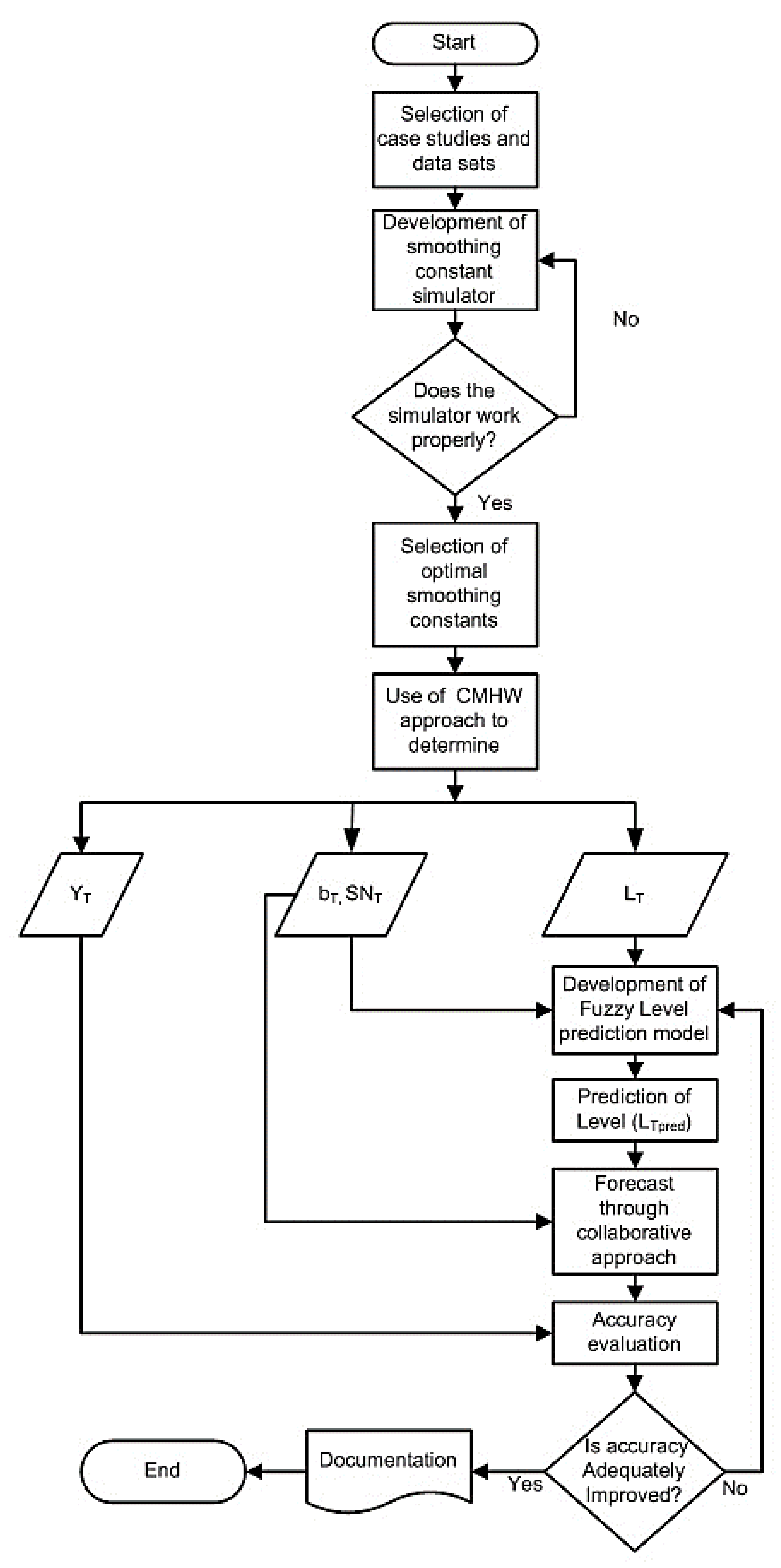
3. Proposed Methodology

The approach presented in this research is intended to propose a collaborative Holt-Winters model for probable exclusion of the effect of stationary means and to make forecasting for seasonal demand more accurate. In this context, the values of appropriate smoothing constants are attained by simulating the historical demand data through an encoded program in MATLAB (R2009b, MathWorks, Natick, MA, USA) to be termed the smoothing constant simulator. Meanwhile, the initial values of the level and growth rate are estimated by the least square method. The initial values of the seasonal components are estimated by de-trending the time-series data, calculating the mean of the de-trended data for each period of chosen seasonal length, and then normalizing the obtained mean values to unity by using the correction factor [27].

All these values are used in determining the time-series parameters such as the level (L_T), growth rate (b_T) and seasonality (SN_T) as well as the forecast (Y_T) by the conventional multiplicative Holt-Winters method. Moreover, the determined values of three parameters would also help to estimate the error (E_L) that is perceived to be magnified by the stationary nature of the initial values. In the fuzzy logic-based level prediction model the parameters L_T, b_T, SN_T and the actual demand Y_T are taken as input variables, while the values of the predicted level (L_Tpred) is considered as the output. A Mamdani fuzzy inference system is applied to contemplate the judgmental knowledge and the relationships established between the variables by means of IF–THEN rules. A de-fuzzification method is employed to obtain the non-fuzzy levels (L_Tpred) which are embedded into the multiplicative Holt-Winters method to obtain the collaborative multiplicative Holt-Winters (Coll-MHW) model-based forecasted demand (Y_Tc). Finally, the accuracy of our proposed collaborative model is assessed by comparing the MAD, MSE and the coefficient of determination for real-life industrial data and two case studies extracted from literature. A brief summary of the research methodology is depicted in Figure 1 by a flow diagram.

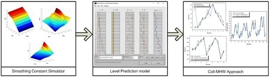
4. Development Stages of the Proposed Approach

As stated earlier, the proposed collaborative forecasting approach consists of a number of successive steps such as introduction of the conventional multiplicative Holt-Winters method, definition of the optimal smoothing constants, determination of the parametric values and forecasted demand, development of the fuzzy logic-based model, and adjustment of the predicted parameter level. All of these steps are discussed comprehensively in the following subsections.

4.1. Development Stages of the Proposed Approach

The multiplicative Holt-Winters model for seasonal demand forecasting consists of an iterative process by incorporating the estimated level (L_T) defined as:

$$L_T=\alpha (D_T/S{N}_{T-l})+(1-\alpha )(L_{T-1}+b_{T-1})$$

(1)

Here, D_T is the actual demand for period T, SN_T−l represents the seasonal index for period T − l, where l denotes the seasonal length, and b_T is the growth rate expressed as:

$$b_T=\beta (L_T-L_{T-1})+(1-\beta )b_{T-1}$$

(2)

In the Holt-Winters method, the seasonal factors are updated at each iteration. Thus, SN_T and SN_T−l, the seasonal indices respectively for the periods T and T − l, are updated by using the following equation:

$$S{N}_T=\gamma (D_T/L_T)+(1-\gamma )S{N}_{T-l}$$

(3)

Generally, starting with the data of a specific period, the Holt-Winters method is able to forecast for the next one or more periods denoted as τ steps. Thus, for example, τ = 3 means that it is possible to forecast for three periods, from period T to T + 1, T + 2 and T + 3. The τ step ahead of forecasted demand (Y_T+τ) can be exposed as:

$$Y_{T+\tau }=(L_T+\tau b_T)S{N}_{T+\tau -l}$$

(4)

So, one step ahead forecasted demand reflecting τ = 1 can be derived from Equation (4) and presented as Equation (5). The error, E_T(L) can be determined by Equation (6). This equation represents a computational process to measure the deficit in estimating the level parameter for each incremental time step, T. In other words, the error, E_T(L) expresses the de-seasonalized and de-trended one-step-ahead likelihood deficit which is used for training the rule base of the fuzzy inference system.

$$Y_{T+1}=\left(L_T+b_T\right)S{N}_{T+1-l}$$

(5)

$$E_{T\left(L\right)}=\left(\left(D_T/S{N}_{T-l}\right)-b_T\right)-L_T$$

(6)

As mentioned earlier, the three smoothing constants (α, β, and γ), also known as the trios and used in the conventional multiplicative Holt-Winters method, are often ascertained subjectively or by using some iterative techniques. In this work, the optimal values of the trios are determined by simulation through a coded program in MATLAB.

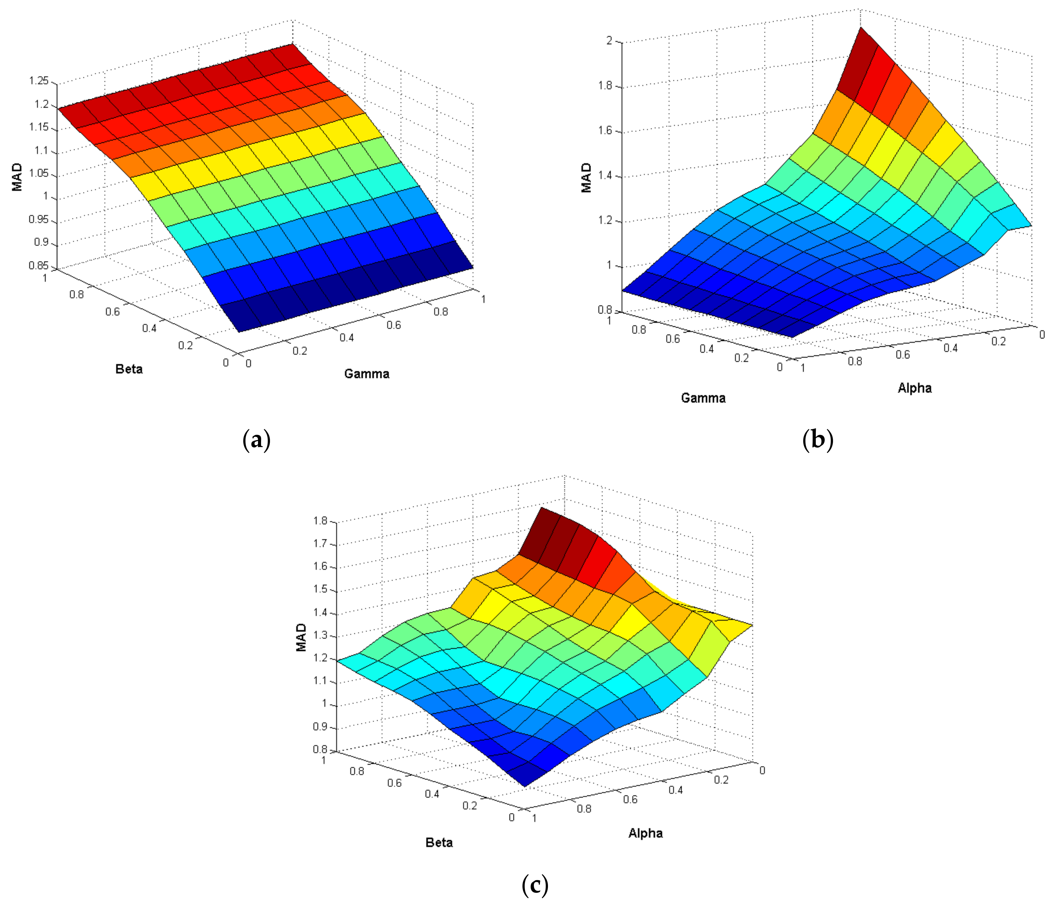
4.2. Development Process of Smoothing Constant Simulator

To determine the optimal values of the trios (α, β, γ) as the smoothing constants within a range of [0, 1], having an incremental step of 0.1, an algorithm is formulated and a program coded in MATLAB, the main steps of which are stated below:

The Pseudo code of Smoothing Constant Simulator is given as follows:

1.   Input: dataset 2.   Initialize parameters 3.   FOR α = 0 to 1 step 0.1 4.        FOR β = 0 to 1 step 0.1 5.           FOR γ = 0 to 1 step 0.1 6.             Calculate first step ahead forecast: 7.             Multiplicative Holt-Winters 8.             Calculate mean absolute deviation: MAD 9.             END FOR 10.        END FOR 11.    END FOR 12.  Find optimum α, β and γ correspond to minimum value of MAD 13.  OUTPUT: Optimum α, β and γ.

4.3. Development Process of Smoothing Constant Simulator

In fuzzy logic-based prediction model the knowledge base, as shown in Figure 2, comprises two components—the data base and the rule base. Usually, the data base is represented by the formulated membership functions, whereas the fuzzy IF–THEN rules form the rule base of the intended knowledge base design. However, the core of this kind of knowledge-based model is the inference engine that employs a set of fuzzy IF–THEN rules to conduct the reasoning mechanism. Generally, the fuzzy reasoning mechanism is defined as a structured procedure for quantifying the conclusion from a given set of rules and conditions.

Nevertheless, a number of fuzzy inference-engine modelling approaches are readily available in literature e.g., the Takagi–Sugeno–Kang (TSK), the Mamdani, etc. Among these, the Mamdani has advantages over others in terms of choosing particular fuzzification and defuzzification procedures, relaxation in representing the membership functions, as well as the wide range of logical operators [55]. Hence, by featuring computational and modelling flexibilities, the Mamdani system is adopted for our research work.

In the process of embedding the defuzzified values of level in the MHW model, computation begins with conversion of the numerical inputs into ‘linguistic variables’ and fixation of their ranges. Upon defining the linguistic variables for fuzzification, the membership functions are also formulated and allocated to each of the variables. By depending on the nature of the models different types of membership functions e.g., triangular, trapezoidal, Gaussian etc. are used in practice. The triangular membership function is adopted for our model due to its simplified features. However, for validation purposes of the developed model in the fuzzy logic tool box, Equation (7) is used to articulate the fuzzification process by representing the input–output membership functions in mathematical form [42,56].

$${\mu }_{triangle}\left(x,c_1,c_2,c_3\right)=\{\begin{array}{l}0;x\le c_1\\ \left(x-c_1\right)/\left(c_2-c_1\right);c_1<x<c_2\\ \left(c_3-x\right)/\left(c_3-c_2\right);c_2<x<c_3\\ 0;x\ge c_3\end{array}$$

(7)

In Equation (7), x represents the value of the input or output variables, whereas c₁, c₂, c₃ are the coefficients of the membership functions. Besides, to build the relationships among input–output variables, several, ‘If–Then’ logical rules are developed for the inference engine. Meanwhile, the fuzzy outputs are derived by aggregating the fuzzy inputs through the logical operators “AND”, where the inference engine brings the compositional effects by incorporating the ‘If–Then’ rules. Then the non-fuzzy values of the desired output are obtained by Equation (8) [56,57].

$$L_{Tpred}^{crisp}=\left({\displaystyle \sum {\mu }_i{a}_i}\right)/{\displaystyle \sum {\mu }_i}$$

(8)

where a_i represents the position of the respective singleton in the respective universe and μ_i stands for the firing strength of the truth degree of the respected rules.

4.4. Estimation of the Parameter Level (LTpred) and the Forecast

Similar to the procedure followed by Hossain et al. [57], the level (L_Tpred) obtained from the fuzzy logic tool box is validated initially by comparing with the values found mathematically. The validated values are then embedded in the conventional MHW method to compute the collaborative multiplicative Holt-Winters (Coll-MHW) model-based forecasted demand (Y_Tc) by applying Equation (9).

$$Y_{Tc}=\left(L_{Tpred}+b_T\right)S{N}_T$$

(9)

4.5. Accuracy Assessment

To judge the accuracy of the forecasting approaches, several benchmarking indicators such as mean absolute deviation (MAD) or mean absolute error (MAE), mean squared error (MSE), mean absolute percent error (MAPE), root mean square error (RMSE) are quite common and adopted in [58,59,60,61]. However, for assessing the strength of our proposed approach, the MAD, the MSE and the coefficient of determination were determined and compared with those obtained through the conventional Holt-Winters method. The equations for the three metrics are as follows [57,58,60,62,63]:

$$MAD={\displaystyle \sum \left|error\right|}/n$$

(10)

$$MSE={\displaystyle \sum {\left(error\right)}^2}/n$$

(11)

$$R^2=1-\frac{{\displaystyle \sum _{i=1}^n\left(y_i-{\widehat{y}}_i\right)}}{{\displaystyle \sum _{i=1}^n\left(y_i-{\overline{y}}_i\right)}}$$

(12)

5. Application of Our Proposed Approach

As mentioned earlier, three case studies are adopted to demonstrate and validate the applicability of our proposed approach. These cases are based on (a) demand data for transformer tanks collected from a local manufacturer; (b) average sales data of a Slovenian company (i.e., Danfoss District Heating) as extracted from literature [36]; and (c) demand data for plastic bags of a manufacturer in south of Spain as extracted from the literature [41]. The whole process is discussed step by step in the following sections.

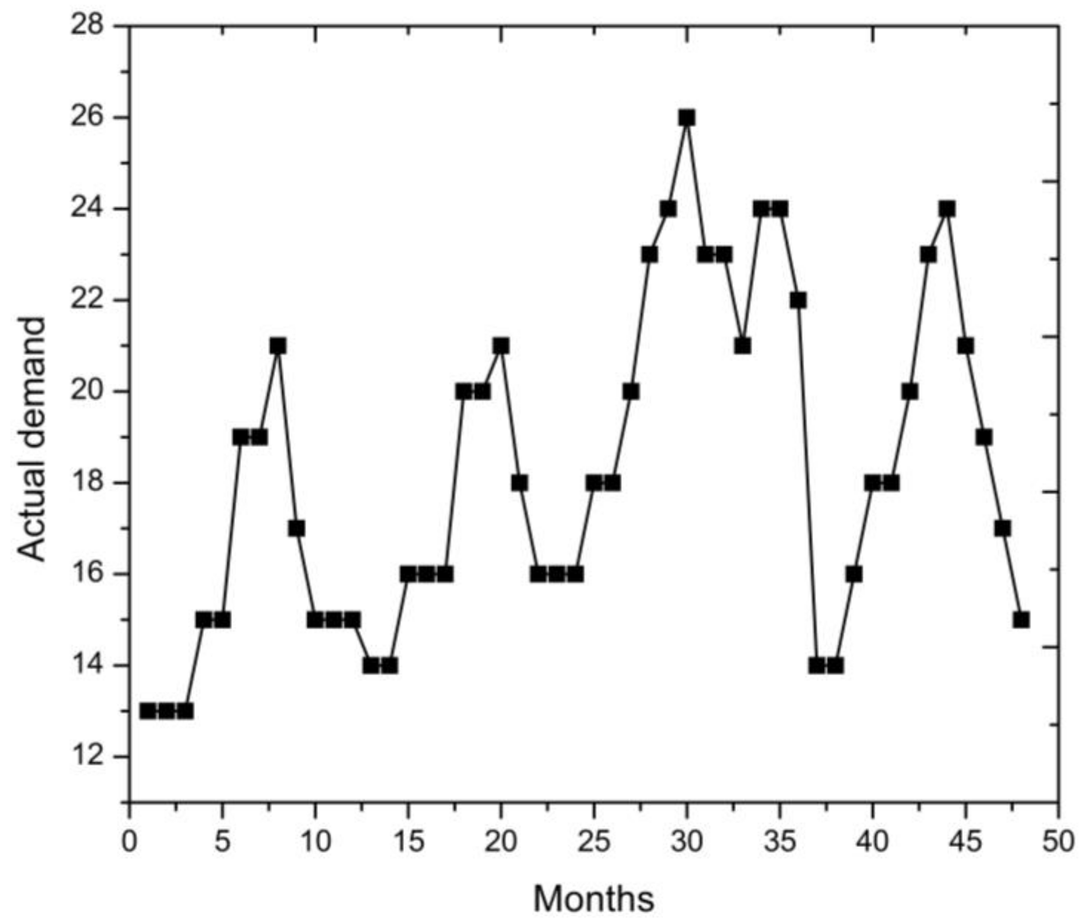
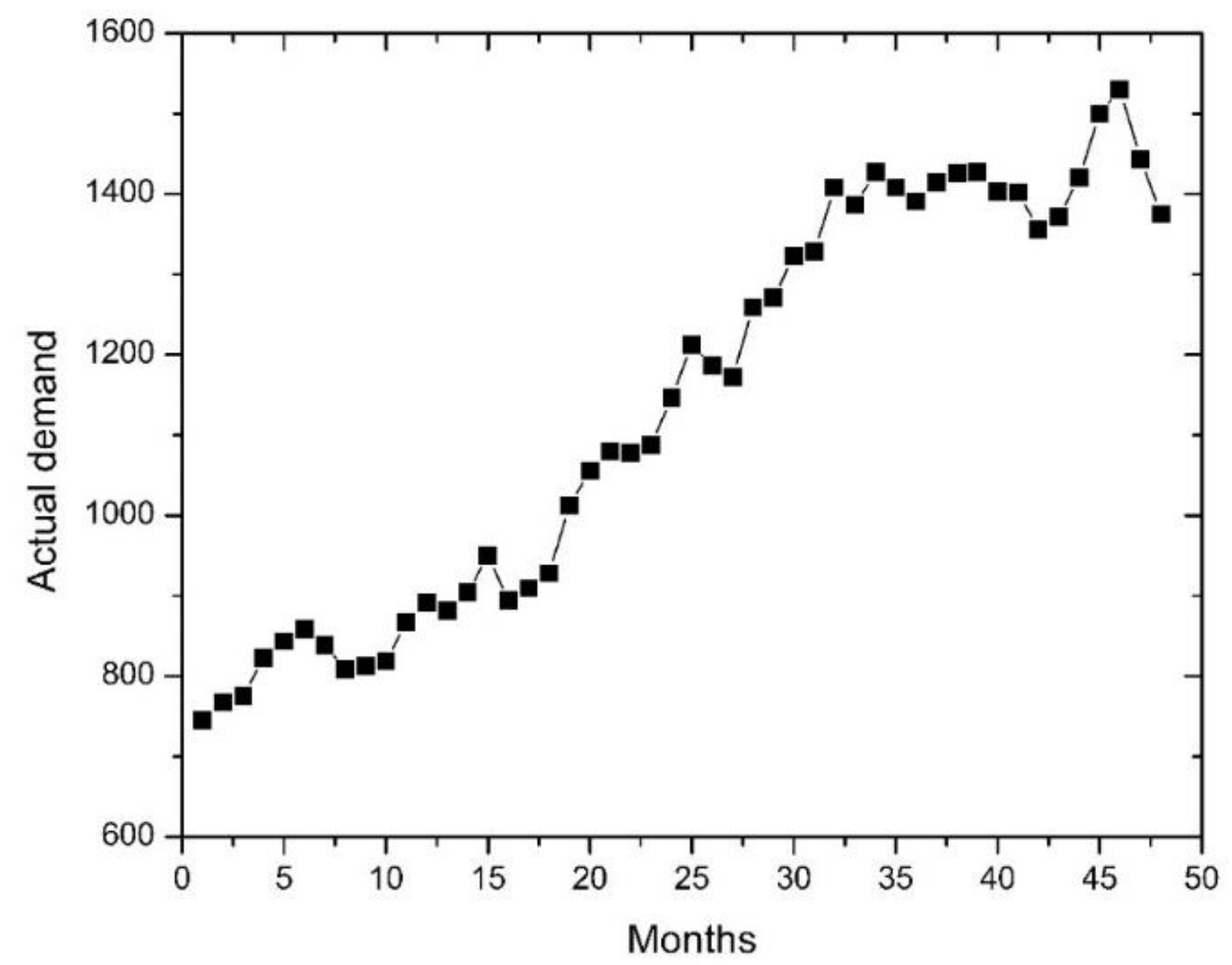
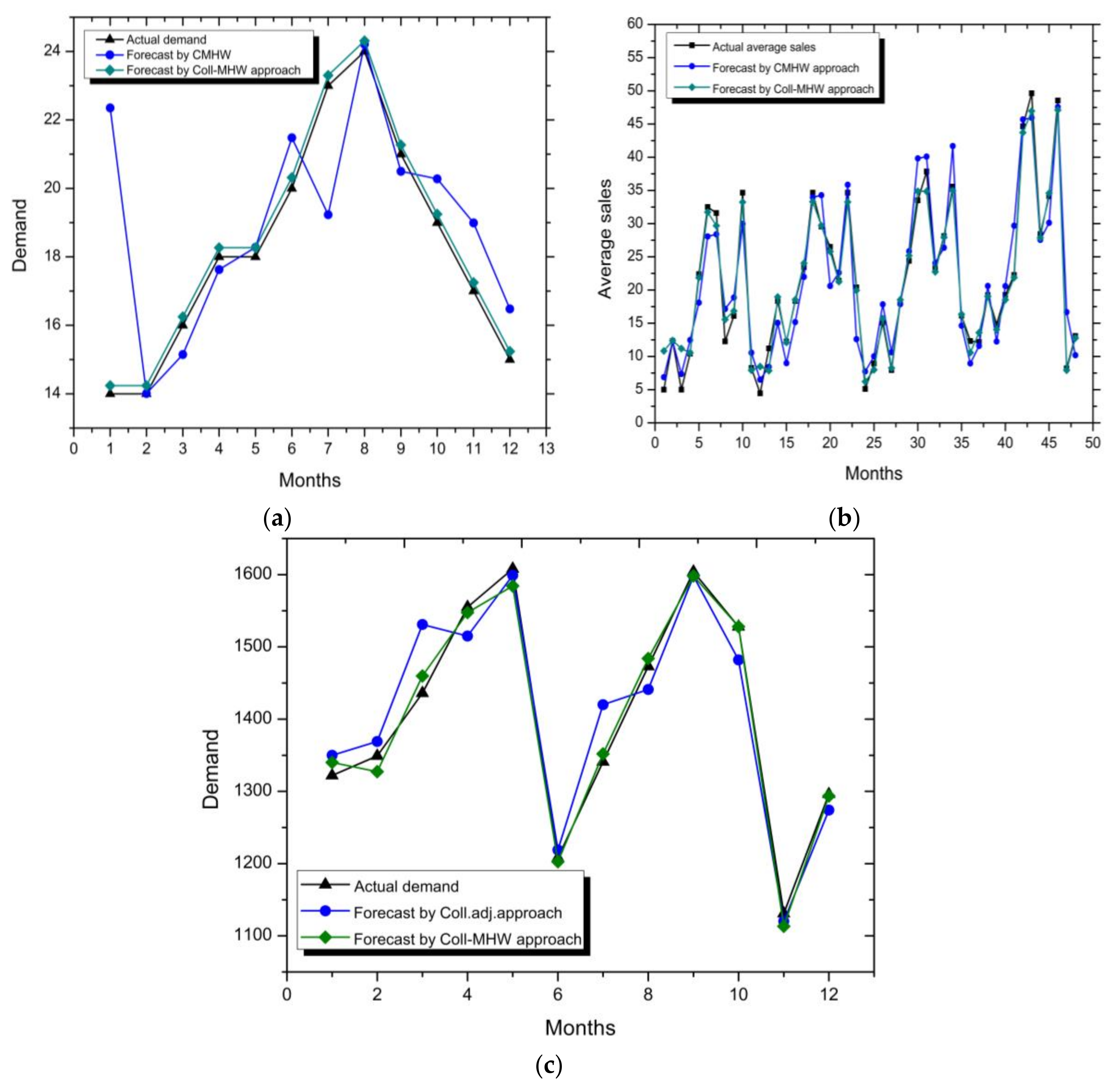
5.1. Case Study-1: Demand Data for Transformer Tanks

The demand data collected from a transformer tank manufacturing company are adopted to validate the proposed methodology. The company mainly produces three types of distribution transformer tanks such as 1000 KV, 750 KV and 500 KV. Among the three models, the 750 KV transformer tank is found to be the vital item for the company. Since the management reviews its production plan at the end of each month, the monthly demand for 750 KV transformer tanks is considered in this study. As presented in Figure 3, the historical records of monthly demand for transformer tanks over the past four years ranging from 2010 to 2013 were revealed by the company. The first three years’ data are used for the training and/or prediction model development purpose while the remaining data are used to test the proposed approach. However, prior to forecast, it is common to examine a time series for characterizing the presence of different demand patterns such as the randomness, trend, seasonality and cyclical behavior. In this context, a scatter diagram of time series representing the demand for 750 KV transformer tanks as shown in Figure 3 reveals an overall uprising trend with multiplicative seasonality.

5.1.1. Determination of the Smoothing Constants

MATLAB coding is used to simulate and determine the best trio of smoothing constants. As a primary objective of the simulation, the best combination of trio was selected against the lower MAD values of the forecast. Optimized values of the trio (α, β and γ) are secured by converging the MAD to its lowest possible value. The converging behavior of MAD is demonstrated in Figure 4a–c, respectively, for the optimum values of α, β and γ.

Figure 4a presents the results of the simulation in which the MAD values are changed in a line with the variation of β and γ while α remains fixed at its optimal value (α = 1). Figure 4b illustrates the effect of α and γ on MAD values with a fixed value of the variable β (β = 0), whereas Figure 4c shows the converging behavior of MAD with respect to α and β for a constant value of 0.2 for γ. It can also be seen that in all of these three exhibits, the MAD is converging to its unique minimal value of 0.89. Hence, the optimum values of the trio (α, β and γ) as obtained through simulation are 1.0, 0.0 and 0.2, respectively.

5.1.2. Determination of the Initial Values

Once the optimum values of the trio (α, β and γ) are obtained, the level (L_T), the growth rate (b_T), the seasonal parameter (SN_T), the forecasted demand (Y_T), and the error (E_T(L)) are computed respectively by using Equations (1)–(6). The computed values are presented in

Table 1. Parametric values based on conventional Holt-Winters approach.

Year	Parameter	Months
		January	February	March	April	May	June	July	August	September	October	November	December
Year 1	DT	13	13	13	15	15	19	19	21	17	15	15	15
	bT	0.27	0.27	0.27	0.27	0.27	0.27	0.27	0.27	0.27	0.27	0.27	0.27
	LT	14.54	14.78	13.88	14.76	14.76	15.90	16.80	17.87	17.16	15.88	16.10	16.86
	SNT	0.89	0.88	0.94	1.02	1.05	1.19	1.13	1.17	0.99	0.94	0.9316	0.89
	YT	12.18	13.03	14.09	14.38	15.28	17.95	18.29	20.06	17.99	16.47	15.04	14.57
	ET(L)	0.92	−0.03	−1.16	0.61	−0.27	0.88	0.63	0.80	−0.98	−1.55	−0.04	0.49
Year 2	DT	14	14	16	16	16	20	20	21	18	16	16	16
	bT	0.27	0.27	0.27	0.27	0.27	0.27	0.27	0.27	0.27	0.27	0.27	0.27
	LT	15.66	15.91	17.089	15.75	15.74	16.74	17.69	17.87	18.17	16.94	17.18	17.98
	SNT	0.89	0.88	0.94	1.02	1.02	1.19	1.13	1.17	0.99	0.94	0.93	0.89
	YT	15.31	14.01	15.15	17.63	16.28	19.13	19.23	21.09	17.97	17.42	16.03	15.52
	ET(L)	−1.47	−0.01	0.90	−1.61	−0.27	0.73	0.68	−0.08	0.03	−1.50	−0.03	0.54
Year 3	DT	18	18	20	23	24	26	23	23	21	24	24	22
	bT	0.27	0.27	0.27	0.27	0.27	0.27	0.27	0.27	0.27	0.27	0.27	0.27
	LT	20.13	20.46	21.36	22.64	23.61	21.76	20.34	19.58	21.20	25.41	25.76	24.72
	SNT	0.89	0.88	0.94	1.01	1.05	1.19	1.13	1.17	0.99	0.94	0.93	0.89
	YT	16.32	17.95	19.41	21.97	23.28	28.53	24.91	24.21	19.66	20.28	23.92	23.16
	ET(L)	1.88	0.06	0.63	1.01	0.71	−2.12	−1.69	−1.03	1.36	3.94	0.09	−1.31

.

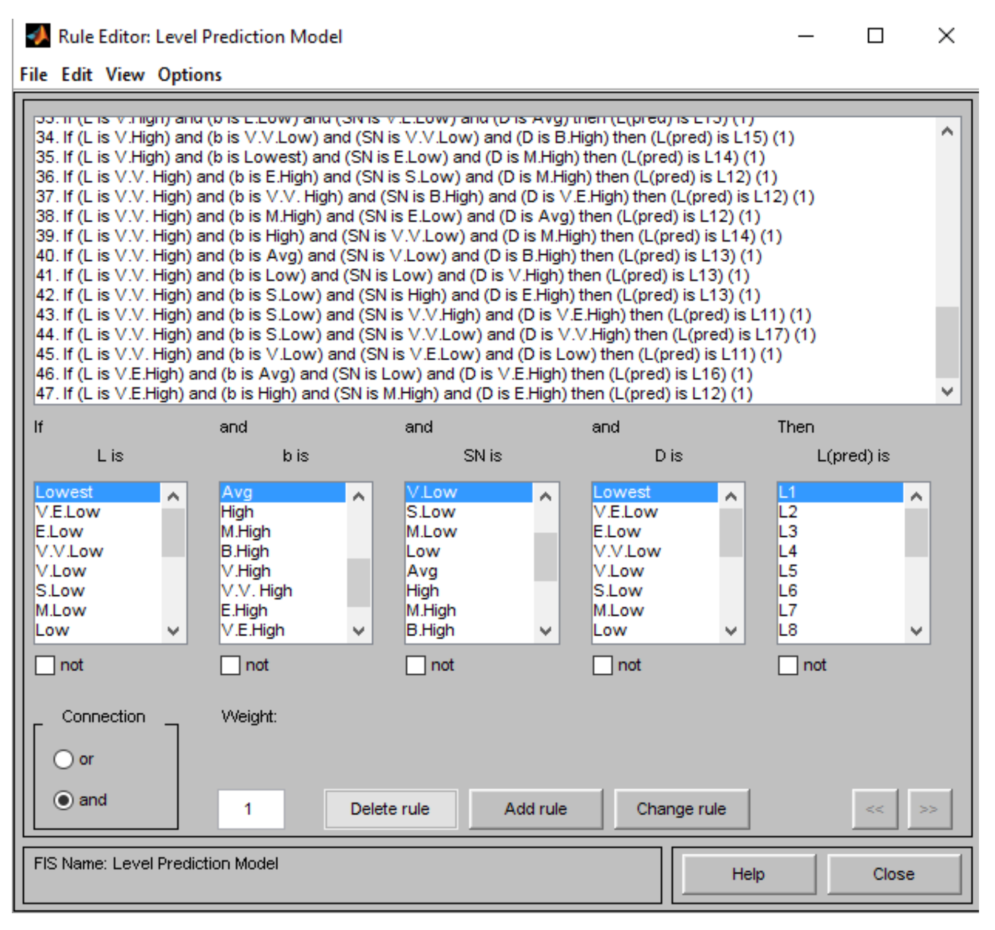
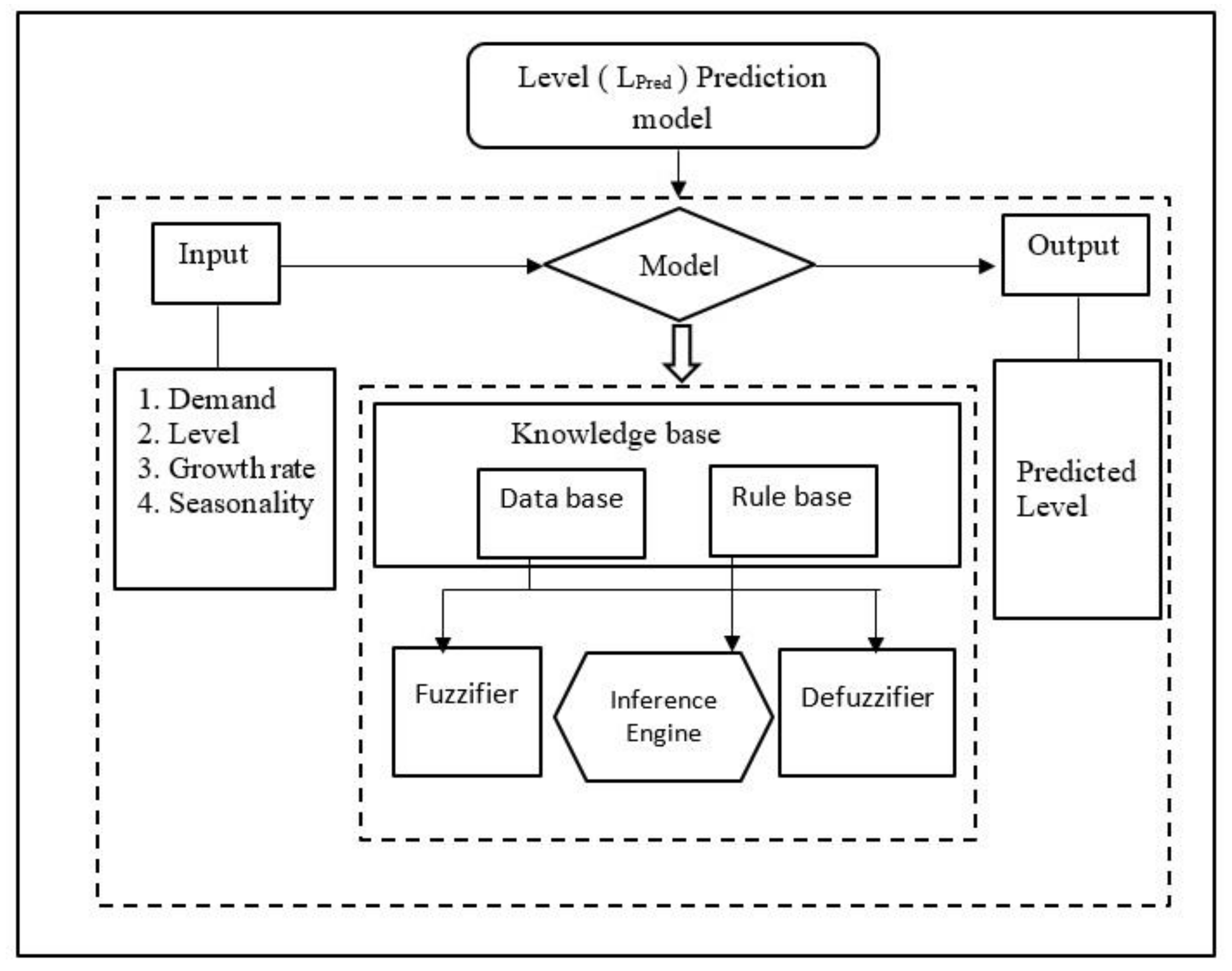
5.1.3. Development of Level Prediction Model

In practice, the Holt-Winters method has been recognized to have relatively higher accuracy and reliability compared to other conventional forecasting approaches. However, the potential lack caused by the consideration of stationary initial values in its recursion process has left scope for incorporating artificial intelligence to improve the forecasting accuracy. In this context, a level prediction model is built via a fuzzy logic-based model. Salient steps in the procedure are described in the following sections.

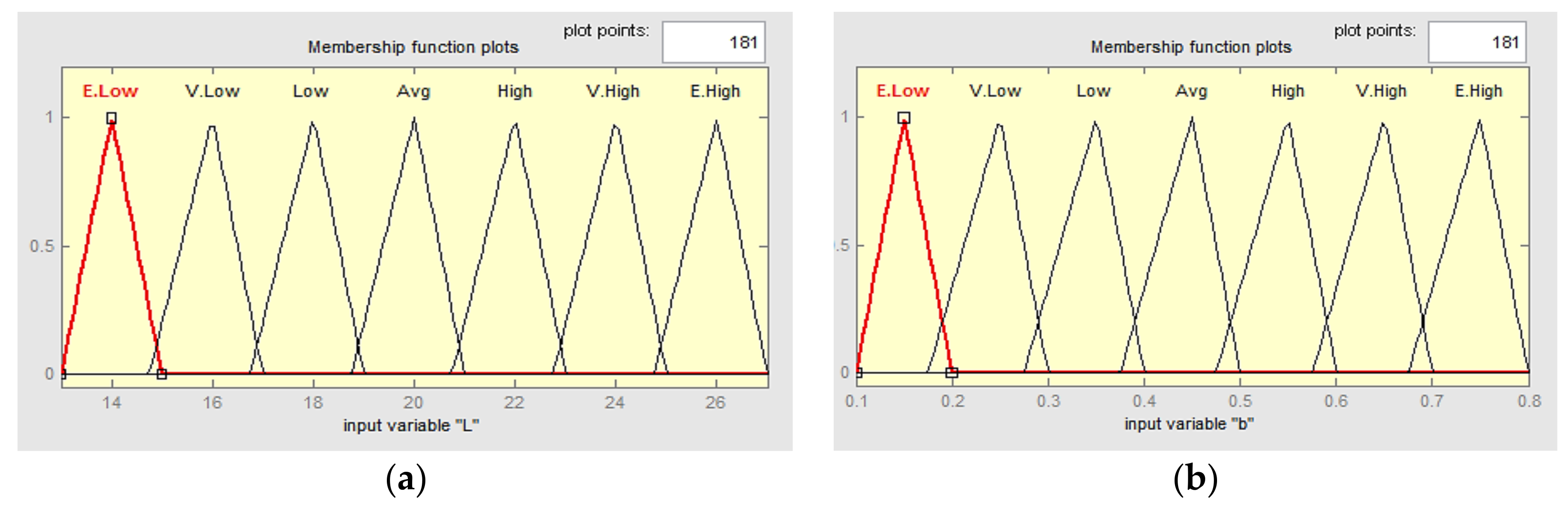
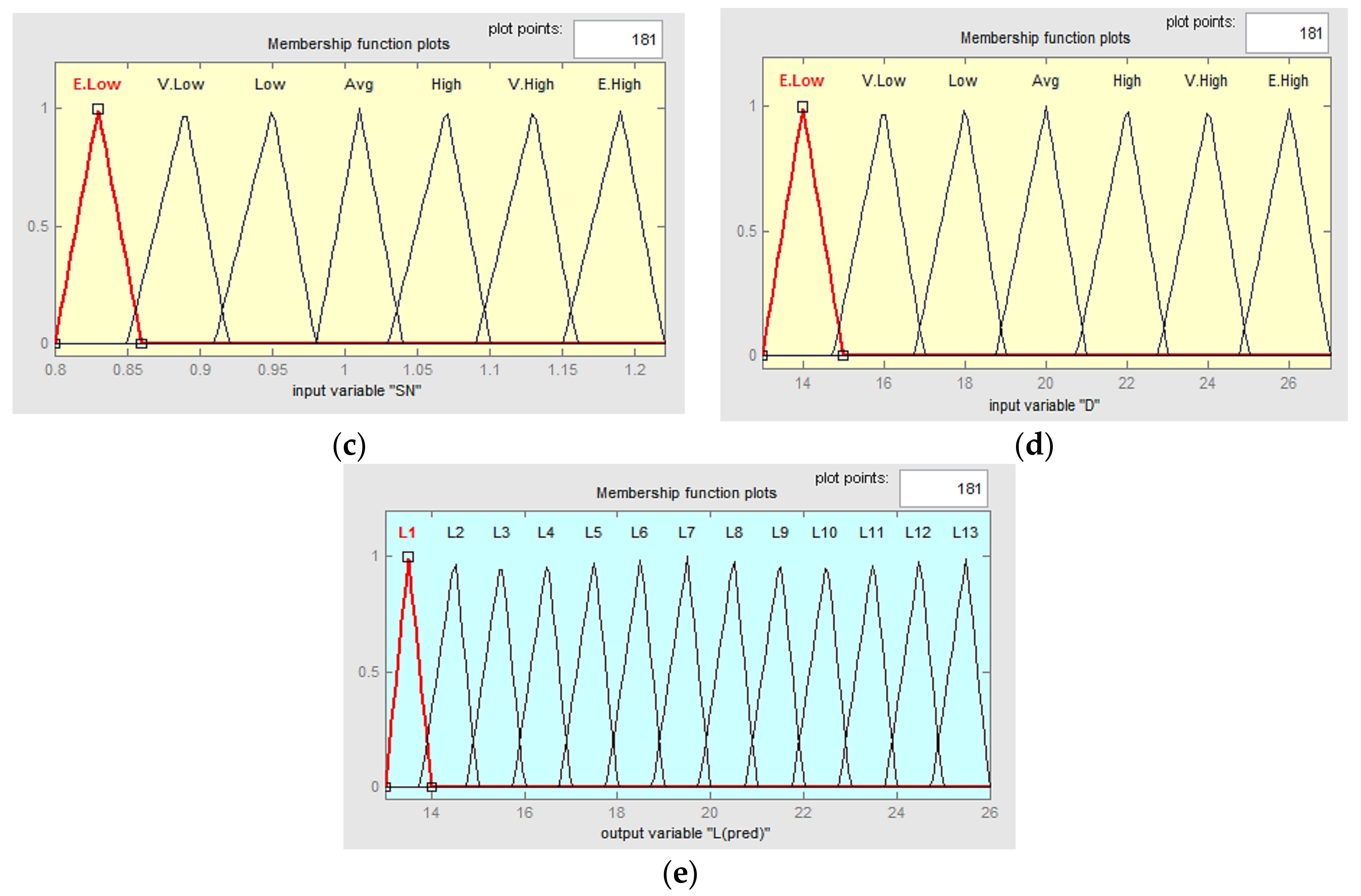
Choice of Inference Mechanism and Variables

In this research, the developed fuzzy logic-based model is implemented in the Fuzzy Logic Toolbox of MATLAB R2009b where the Mamdani inference system is chosen for predicting the parameter level (L_Tpred). It is also necessary to define the input and output variables since their interrelations will materialize the objective(s) of the fuzzy logic-based model. Input variables i.e., the demand (D_T), the level (L_T), the growth rate (b_T), the seasonal parameter (SN_T), and output variables i.e., the predicted level (L_Tpred), in the MATLAB platform are exhibited by Figure A1 in Appendix A.

Fuzzification and Formulation of Membership Functions

In the fuzzification stage, the values of all the linguistic variables, as shown in

Table 2. Linguistic variables, their associated values and ranges.

Variables	Linguistic Variables	Linguistic Values	Ranges
Input	Level (LT)	E. Low	13~15
		V. Low	14.75~17
		Low	16.75~19
		Avg	18.75~21
		High	20.75~23
		V. High	22.75~25
		E. High	24.75~27
	Growth rate (bT)	E. Low	0.1~0.2
		V. Low	0.175~0.3
		Low	0.275~0.4
		Avg	0.375~0.5
		High	0.475~0.6
		V. High	0.575~0.7
		E. High	0.675~0.8
	Seasonal parameter (SNT)	E. Low	0.8~0.84
		V. Low	0.837~0.88
		Low	0.875~0.92
		Avg	0.9175~0.96
		High	0.9575~1
		V. High	0.9975~1.4
		E. High	1.375~1.8
	Demand (DT)	E. Low	13~15
		V. Low	14.75~17
		Low	16.75~19
		Avg	18.75~21
		High	20.75~23
		V. High	22.75~25
		E. High	24.75~27
Output	Predicted level (LTpred)	L1	13~14
		L2	13.75~15
		L3	14.75~16
		L4	15.75~17
		L5	16.75~18
		L6	17.75~19
		L7	18.75~20
		L8	19.75~21
		L9	20.75~22
		L10	21.75~23
		L11	22.75~24
		L12	23.75~25
		L13	24.75~26

, are fuzzified with the aid of membership functions. Usually the membership functions are considered as the core of fuzzy logic-based modelling as they have a direct influence on the strength and weakness of the model [64,65]. Among the different types of membership functions, the triangular one is selected for the fuzzification purpose due to its ease of construction and versatility for system representations [66].

However, in this intended development of the fuzzy logic model, the fuzzification of the linguistic parameters is conducted by the following functions:

$$L_T\left(i_1\right)=\{\begin{array}{l}{i}_1;13\le i_1\le 27\\ 0;\mathrm{Otherwise}\end{array}$$

(13)

$$b_T\left(i_2\right)=\{\begin{array}{l}{i}_2;0.1\le i_2\le 0.8\\ 0;\mathrm{Otherwise}\end{array}$$

(14)

$$S{N}_T\left(i_3\right)=\{\begin{array}{l}{i}_3;0.8\le i_3\le 1.8\\ 0;\mathrm{Otherwise}\end{array}$$

(15)

$$D_T\left(i_4\right)=\{\begin{array}{l}{i}_4;13\le i_4\le 27\\ 0;\mathrm{Otherwise}\end{array}$$

(16)

$$L_{Tpred}\left(o_1\right)=\{\begin{array}{l}{o}_1;13\le o_1\le 26\\ 0;\mathrm{Otherwise}\end{array}$$

(17)

where, i₁, i₂, i₃, i₄, o₁ are the variables related to the level, growth rate, seasonality, actual demand and predicted level, respectively. The triangular fuzzy numbers for the input variables i.e., the demand (D_T), level (L_T), growth rate (b_T), seasonal parameter (SN_T), and the output variables i.e., the predicted level (L_Tpred) are given in

Table 3. Fuzzy numbers for the input and output variables.

Variable Name	Fuzzy Numbers	Variable Name	Fuzzy Numbers
Level, LT	E. Low = (13, 14, 15; 1) V. Low = (14.75, 16, 17; 1) Low= (16.75, 18, 19; 1) Avg= (18.75, 20, 21; 1) High= (20.75, 22, 23; 1) V. High = (22.75, 24, 25; 1) E. High = (24.75, 26, 27; 1)	Seasonal parameter (SNT)	E. Low = (0.8, 0.82, 0.84; 1) V. Low = (0.837, 0.86, 0.88; 1) Low = (0.875,0.9, 0.92; 1) Avg = (0.9175, 0.94, 0.96; 1) High = (0.9575, 0.98,1; 1) V. High = (0.9975, 1.2, 1.4; 1) E. High = (1.375, 1.6, 1.8; 1)
Growth Rate, bT	E. Low = (0.1, 0.15, 0.2; 1) V. Low = (0.175, 0.25, 0.3; 1) Low = (0.275, 0.35, 0.4; 1) Avg = (0.375, 0.45, 0.5; 1) High = (0.475, 0.55, 0.6; 1) V. High = (0.575, 0.65, 0.7; 1) E. High = (0.675, 0.75, 0.8; 1)	Predicted Level (LTpred)	L1 = (13, 13.5, 14; 1) L2 = (13.75, 14.5, 15; 1) L3 = (14.75, 15.5, 16; 1) L4 = (15.75, 16.5, 17; 1) L5 = (16.75, 17.5, 18; 1) L6 = (17.75, 18.5, 19; 1) L7 = (18.75, 19.5, 20; 1) L8 = (19.75, 20.5, 21; 1) L9 = (20.75, 21.5, 22; 1) L10 = (21.75, 22.5, 23; 1) L11 = (22.75, 23.5, 24; 1) L12 = (23.75, 24.5, 25; 1) L13 = (24.75, 25.5, 26; 1)
Actual Demand, DT	E. Low = (13, 14, 15; 1) V. Low = (14.75, 16, 17; 1) Low = (16.75, 18, 19; 1) Avg = (18.75, 20, 21; 1) High = (20.75, 22, 23; 1) V. High = (22.75, 24, 25; 1) E. High = (24.75, 26, 27; 1)

by characterizing the definition as well as the properties presented in the work of Chu and Tsao [67].

However, to demonstrate this fuzzification process through mathematical interpretation [42,57,68], the membership functions for the input and output variables are worked out by using Equation (7). Figure A2a–e as provided in Appendix A illustrate all the developed membership functions in the MATLAB platform. However, for fuzzification and/or articulation of the membership functions, the associated values of the coefficients of the entire input and output variables are shown in

Table 4. Coefficients of membership functions for variables.

Variable	Linguistic Variables	Type	Coefficient
			C1	C2	C3
LT	E. Low	Triangular	13	14	15
	V. Low	Triangular	14.75	16	17
	Low	Triangular	16.75	18	19
	Avg	Triangular	18.75	20	21
	High	Triangular	20.75	22	23
	V. High	Triangular	22.75	24	25
	E. High	Triangular	24.75	26	27
bT	E. Low	Triangular	0.1	0.15	0.2
	V. Low	Triangular	0.175	0.25	0.3
	Low	Triangular	0.275	0.35	0.4
	Avg	Triangular	0.375	0.45	0.5
	High	Triangular	0.475	0.55	0.6
	V. High	Triangular	0.575	0.65	0.7
	E. High	Triangular	0.675	0.75	0.8
SNT	E. Low	Triangular	0.8	0.82	0.84
	V. Low	Triangular	0.837	0.86	0.88
	Low	Triangular	0.875	0.9	0.92
	Avg	Triangular	0.9175	0.94	0.96
	High	Triangular	0.9575	0.98	1
	V. High	Triangular	0.9975	1.2	1.4
	E. High	Triangular	1.375	1.6	1.8
DT	E. Low	Triangular	13	14	15
	V. Low	Triangular	14.75	16	17
	Low	Triangular	16.75	18	19
	Avg	Triangular	18.75	20	21
	High	Triangular	20.75	22	23
	V. High	Triangular	22.75	24	25
	E. High	Triangular	24.75	26	27
LTpred	L1	Triangular	13	13.5	14
	L2	Triangular	13.75	14.5	15
	L3	Triangular	14.75	15.5	16
	L4	Triangular	15.75	16.5	17
	L5	Triangular	16.75	17.5	18
	L6	Triangular	17.75	18.5	19
	L7	Triangular	18.75	19.5	20
	L8	Triangular	19.75	20.5	21
	L9	Triangular	20.75	21.5	22
	L10	Triangular	21.75	22.5	23
	L11	Triangular	22.75	23.5	24
	L12	Triangular	23.75	24.5	25
	L13	Triangular	24.75	25.5	26

.

Meanwhile, as adopted by [69], the membership functions and the linguistic fuzzy sets of a particular input L_T are also deduced by using Table 4, Equation (7), Equation (13) and presented through Equations (18)–(24). The membership functions for the remaining input and output variables are also developed in the same manner as shown by Equations (18)–(24).

$${\mu }_{E.Low}\left(L_T\right)=\{\begin{array}{l}\frac{x_{}-13}{14-13};13\le x\le 14\\ \frac{15-x}{15-14};14\le x\le 15\\ 0;x>15\end{array}$$

(18)

$${\mu }_{V.Low}\left(L_T\right)=\{\begin{array}{l}\frac{x-14.75}{16-14.75};14.75\le x\le 16\\ \frac{17-x}{17-16};16\le x\le 17\\ 0;x>17\end{array}$$

(19)

$${\mu }_{Low}\left(L_T\right)=\{\begin{array}{l}\frac{x-16.75}{18-16.75};16.75\le x\le 18\\ \frac{19-x}{19-18};18\le x\le 19\\ 0;x>19\end{array}$$

(20)

$${\mu }_{Avg}\left(L_T\right)=\{\begin{array}{l}\frac{x-18.75}{20-18.75};18.75\le x\le 20\\ \frac{21-x}{21-20};20\le x\le 21\\ 0;x>21\end{array}$$

(21)

$${\mu }_{High}\left(L_T\right)=\{\begin{array}{l}\frac{x-20.75}{22-20.75};20.75\le x\le 22\\ \frac{23-x}{23-22};22\le x\le 23\\ 0;x>23\end{array}$$

(22)

$${\mu }_{V.High}\left(L_T\right)=\{\begin{array}{l}\frac{x-22.75}{24-22.75};22.75\le x\le 21.87\\ \frac{25-x}{25-24};25\le x\le 24\\ 0;x\ge 25\end{array}$$

(23)

$${\mu }_{E.High}\left(L_T\right)=\{\begin{array}{l}\frac{x-24.75}{26-24.75};24.75\le x\le 26\\ \frac{27-x}{27-26};26\le x\le 27\\ 0;x\ge 27\end{array}$$

(24)

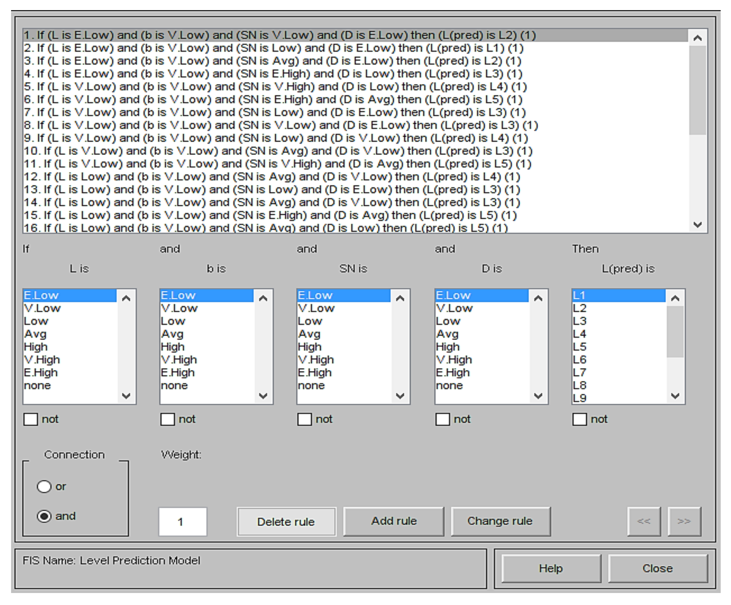
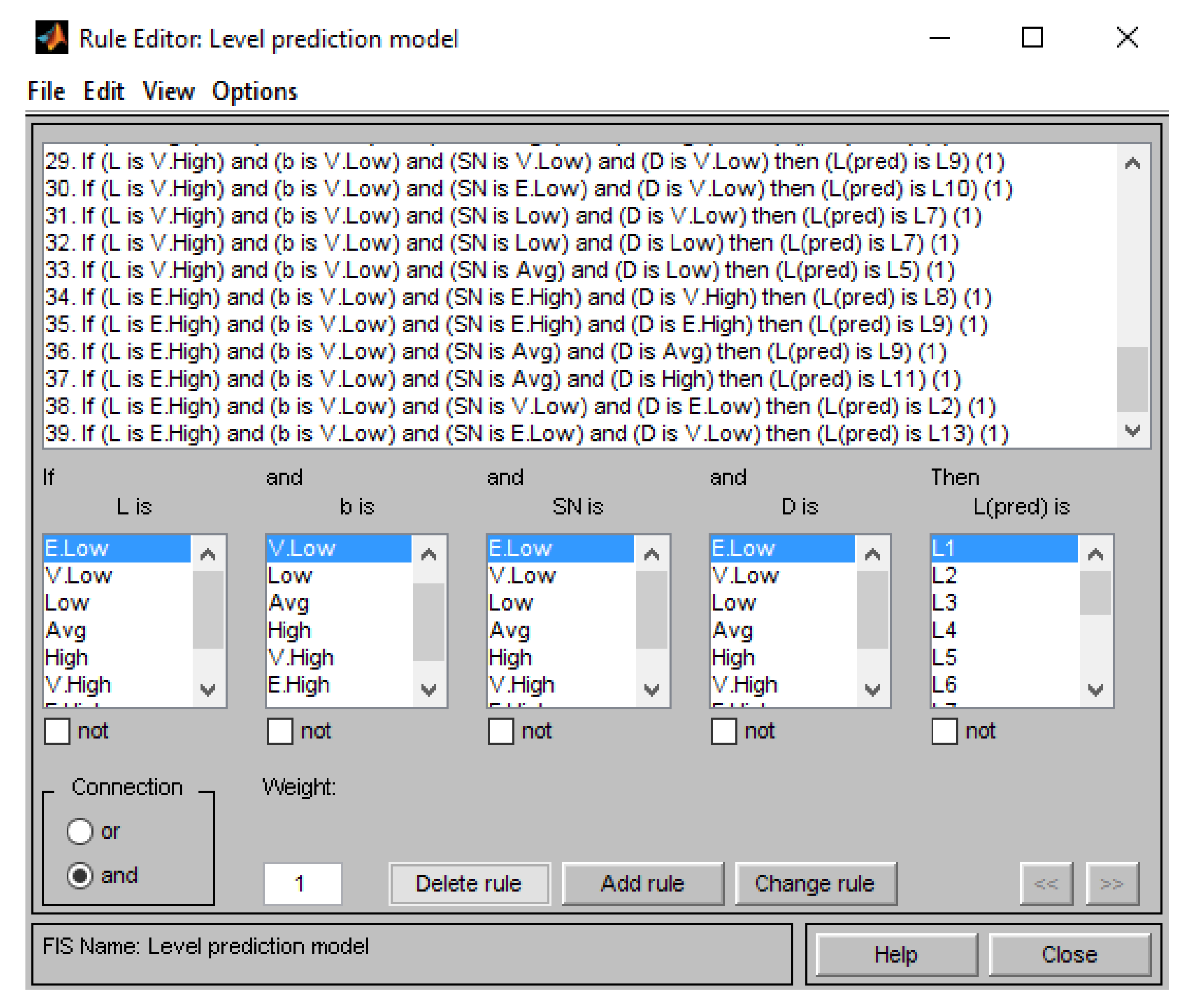
Development of Fuzzy Inference Rules and Process

For Case-1, 30 decision rules, as presented in Figure 5, are formulated and inserted in the fuzzy logic tool box. Each rule has two distinct parts: premise and conclusion. The input variables are interpreted with the premise part as “if” whereas the output variables are taken with conclusion as “then”. To clarify how a rule works, an example is given for one of the decision rules along with the interpretation:

Rule 1: If L = E. low and b = V. low and SN = V. low and D = E. low, then L (pred) = L2. This means that if the level is E. low, growth rate is V. low, seasonality is V. low, demand is E. low; then the predicted level is L2.

After formulating the decision rules and membership functions, the inference process is carried out. In the first step of the inference, the conclusion of each decision rule is derived for a particular input by a comprehensive comparison among the ranges of input variables. At this step of implementation, the logical operator ‘AND’ is used to connect the inputs. The overall conclusion is made by the aggregation of the selected decision rules to a single fuzzy set. This aggregation is carried out by selecting the truth degree of each rule through the min–max operation. Finally, the non-fuzzy values are obtained by de-fuzzifying the fuzzy sets through Equation (8).

To perceive the defuzzification process mathematically and assess the validation of the developed level prediction model on MATLAB [56,57], an example is presented with an input for L_T = 16.74, b_T = 0.27, SN_T = 1.13 and D_T = 20.00 corresponding to the 19th month. The membership functions, the decision rules as well as the rule viewers of the fuzzy logic tool box (as shown in Figure 6) indicate that for the given inputs only the decision rule 11 is fired (i.e., output for this rule is non zero) and all other rules remain in the non-fired (i.e., output of these non-fired rules are zero) position. Similar to what is adopted by Hossain et al. [69], for this particular rule the fuzzy values of the input L_T, b_T, SN_T and D_T are computed by using Equation (7) and the values obtained are as follows:

$${\mathsf{\mu }}_{V.Low}\left(L_T\right)=0.260;{\mathsf{\mu }}_{V.Low}\left(b_T\right)=0.644$$

$${\text{µ}}_{V.High}\left(S{N}_T\right)=1.350;{\mathsf{\mu }}_{Avg}\left(D_T\right)=1.000$$

Whereas, for rule 11, the firing strength (truth value) are determined as follows:

$$\begin{array}{l}{a}_{11}=\min \{{\text{µ}}_{V.Low}\left(L_T\right),{\text{µ}}_{V.Low}\left(b_T\right),\\ {\text{µ}}_{V.High}\left(S{N}_T\right),{\mathsf{\mu }}_{Avg}\left(D_T\right)\}\\ =\min \left(0.260{,}_{}0.644{,}_{}1.350{,}_{}1.00\right)\\ =0.260\end{array}$$

Finally, for the defuzzification, the crisp output of the predicted level is computed as 17.34 by using Equation (8); whereas the developed fuzzy logic-based model in MATLAB as shown in Figure 6, provides an output of 17.4 for the same inputs. This shows that the obtained output of 17.34 is very close compared to the output 17.4 given by the model developed in the MATLAB fuzzy toolbox. By featuring this higher accuracy, the obtained output of the predicted level (L_Tpred) is used to compute the new series of forecasted demand (Y_Tc).

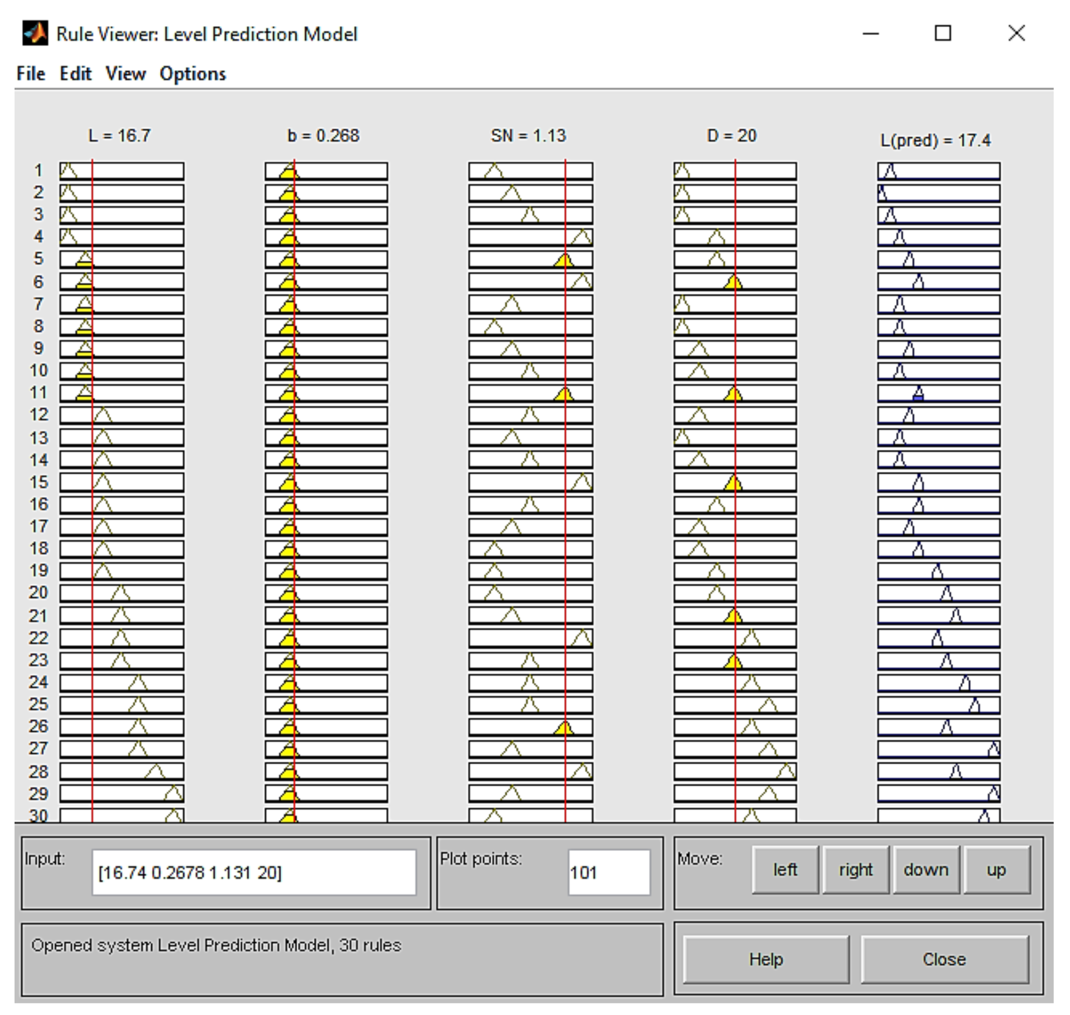
5.1.4. Prediction of Level and Consequent Forecast

At this stage, the new series of collaborative model-based forecasted demand (Y_Tc) for the test set is obtained by using Equation (9). The value of the demand (D_T), level (L_T), predicted level (L_Tpred), forecasted demand (Y_T) and the consequent model-based forecasts (Y_Tc) for the test period are given in

Table 5. Parametric values and forecasts for the test period.

Components	Time Period
	1	2	3	4	5	6	7	8	9	10	11	12
DT	14	14	16	18	18	20	23	24	21	19	17	15
LT	15.66	15.91	17.08	17.71	17.71	16.74	20.34	20.43	21.20	20.11	18.25	16.86
LTpred	15.4	15.4	16.4	17.4	17.4	17.4	19.5	19.5	22.4	21.4	19.5	17.4
YT	22.35	14.01	15.15	17.63	18.28	21.48	19.23	24.21	20.50	20.28	18.99	16.48
YTc	14.24	14.24	16.25	18.27	18.27	20.32	23.30	24.31	21.27	19.25	17.25	15.24

.

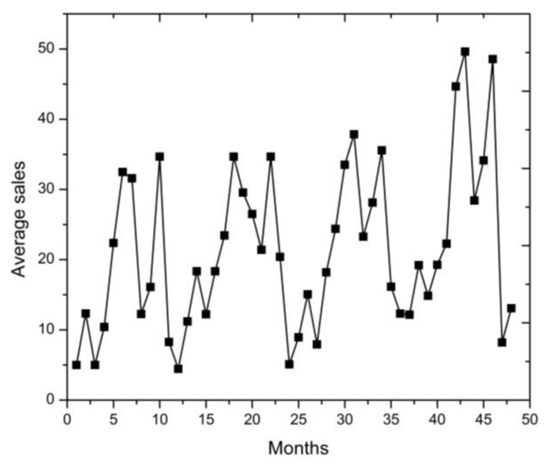
5.2. Case Study-2: Average Sales Data of Danfoss District Heating

The average sales data of 4247 products of a Slovenian company named Danfoss District Heating, which was originally presented by Tratar [36], is adapted in this research for validating and assessing the strength of our proposed collaborative approach. The time series, as shown in Figure 7, represents the monthly average sales data for the time span of four years ranging from 2005 to 2008. The data set also depicts the varying means and the overall uprising trend with multiplicative seasonal patterns.

However, to assess the strength of our proposed collaborative approach, initially the starting values of the level, the growth rate and the seasonal components are estimated. These initial values are incorporated with the conventional multiplicative Holt-Winters method to determine the time-series parameters such as the level (L_T), growth rate (b_T), seasonality (SN_T) as well as the forecast (Y_T). A fuzzy logic-based level prediction model is also developed to attain the output level (L_Tpred). To do so, the Mamdani fuzzy inference system is chosen to contemplate the judgmental knowledge and the relationships established between the variables by means of 39 IF–THEN rules and the logical operator ‘AND’ as shown in Figure 8.

Finally, the de-fuzzification is performed by using Equation (8) to obtain the non-fuzzy levels (L_Tpred) which are embedded into the multiplicative Holt-Winters method to get the Coll-MHW model-based forecasted demand (Y_Tc) through Equation (9).

5.3. Case Study-3: Demand Data for Plastic Bags

In their research, Cheikhrouhou et al. [41] presented a four-year monthly demand data set for plastic bags collected from a manufacturer in the south of Spain. The data set as presented in Figure 9 exhibits the changing means, growth rates and seasonal patterns for which the multiplicative version of the Holt-Winters approach looks to be a relevant for forecasting. From this data set, the first three years’ data (for 2004–2006) are used in the training period to forecast demand for the period of 2007.

To forecast through our proposed collaborative approach, the starting values of the level, the growth rate, the seasonal components and the forecast are estimated initially by the conventional multiplicative Holt-Winters method. In addition, a Mamdani type fuzzy logic-based level prediction model is developed to attain the output level (L_Tpred) through incorporation of 47 IF–THEN rules and logical operator ‘AND’, as shown in Figure 10. Meanwhile, the values of levels (L_Tpred) and forecasted demand (Y_Tc) are obtained by using Equations (8) and (9), respectively. Finally, the accuracy of the forecasted demand for the period of 2007 is assessed by means of MAD and MSE.

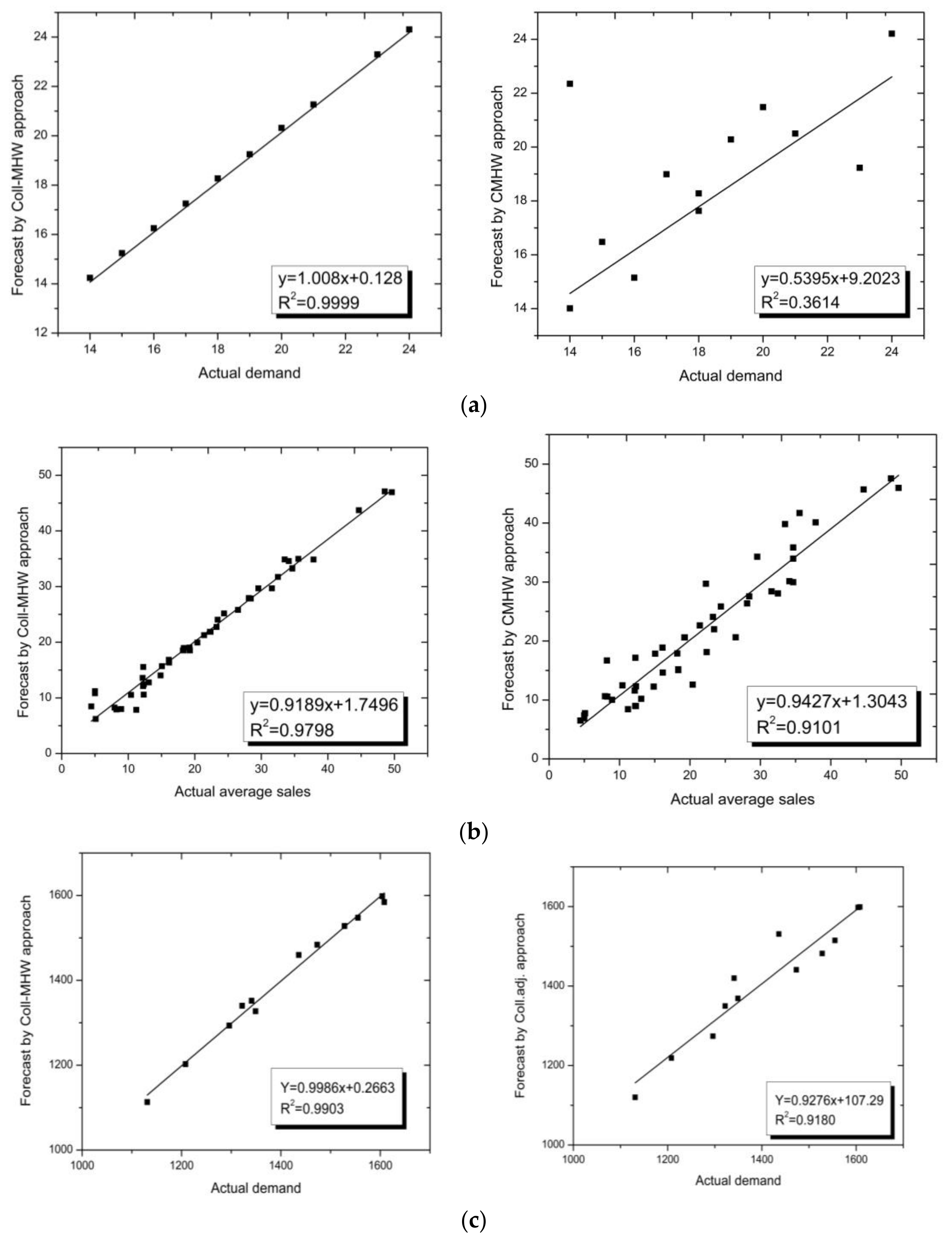
6. Results and Discussions

The forecasted results obtained by means of the Coll-MHW are used to evaluate the MAD, MSE and coefficient of determination as the statistical measures for accuracy assessment.

6.1. Evaluation of the Forecasting Accuracy

To evaluate the forecasting accuracy, measures of performance such as MAD and MSE are used. In this context Equations (10) and (11) are used to determine the values of MAD and the MSE respectively for all the three cases. As presented in

Table 6. Comparison of forecasting accuracy.

Cases	Method Used Earlier	Forecast Error Obtained by Earlier Method		Forecast Error Obtained by Proposed Coll. MHW		Error Reduction
		MAD	MSE	MAD	MSE	MAD	MSE
1	CMHW	1.71	0.65	0.27	0.01	84.21%	98.5%
2	CMHW	9555.75	51,199.94	4972.62	13,757.55	48%	73%
	IMHW	12,269.11	52,261.69			59.5%	73.6%
3	ARIMA	112.2	16,821	12.35	216.92	89%	98%
	Coll. Adj.	33.91	1836.08			63.5%	88%

, the MAD and MSE obtained for the forecast values yielded by the proposed Coll-MHW method outperform all other methods. It is to be noted that MAD and MSE values for Case-1 are evaluated by using the conventional multiplicative Holt-Winters method (CMHW) whereas for Case-2 and Case-3 the values of MAD and MSE are obtained from literature. As stated in the published papers, the forecast values for Case-2 were determined by CMHW and improved multiplicative Holt-Winters method (IMHW), while those for Case-3 were evaluated by ARIMA and collaborative adjusted (Coll. Adj.) models.

It would also be interesting to demonstrate the forecasting performance of the proposed approach for each of the individual periods of time series. In this respect, Figure 11a–c portray a comparative scenario for the three cases. The comparative scenarios as presented in Table 5 and plots in Figure 11a–c consistently reveal the superior performance of our proposed collaborative approach in comparison to the conventional MHW, improved MHW, ARIMA and Coll. Adj. forecasting models.

6.2. Assessing the Coefficient of Determination

Apart from assessment of forecasting accuracy, the coefficient of determination is evaluated to reflect the strength and validation of the models. To check the appropriateness of our proposed model, the values for the coefficient of determination are computed and compared with those for other methods. For this purpose, the transformer tank demand over a period of one year, the average sales of Danfoss District Heating, and the data on plastic bag demand are used as before.

Table 7. Improvement in the coefficient of determination.

Cases	Method Used Earlier	R2 Using Earlier Method	R2 for Proposed Coll-MHW Approach	Improvement
1	CMHW	0.3614	0.9999	63.85%
2	CMHW	0.9101	0.9798	6.97%
3	Coll. Adj.	0.9180	0.9903	7.23%

and Figure 12a–c exhibit the coefficient of determination.

It is to be noted that the coefficient of determination computed by our proposed Coll-MHW approach is compared with those yielded by the CMHW for Case-1 and Case-2 and by the Coll. Adj. for Case-3. Regrettably, it could not be assessed for the ARIMA and IMHW methods due to the absence of the required data. However, as delineated in Table 7 and in Figure 12a–c, the coefficient of determination (R²) values validate the superior performance of our proposed Coll-MHW approach.

7. Conclusions

Irrespective of whether a firm is oriented to services or manufacturing, many operational decisions are highly dependent on the predicted values of certain events or issues. In this context, the role of an appropriate forecasting approach cannot be ignored. Although a prediction can never be perfect, an endeavor is always under way to search for an accurate forecasting approach. The developed collaborative multiplicative Holt-Winters (Coll-MHW) approach as proposed in this paper is facilitated by a fuzzy logic-based prediction model to dynamically estimate the L_T value and embed it into the conventional MHW method. This newly proposed Coll-MHW approach is tested through several case studies and is found to be robust with superior performance. Moreover, our proposed approach does not require the inclusion of any judgmental consideration like transient factors, transferred impact factors, quantum jump factors and trend change factors as quoted by Cheikhrouhou et al. (2011) [41]. So, the proposed Coll-MHW approach is expected to be a potential forecasting method to address multiplicative seasonal demand forecasting problems and to secure its place as an effective tool for prediction. In future, the proposed method is likely to be enriched in an extended, robust form for wider application through the inclusion of lifecycle demand data and AI-like neural network. In this context, the impact of the appropriate choice and adoption of different kinds of membership functions on the performance metrics for this proposed collaborative forecasting model is also kept in mind for an extended scope of future research.

References

1. Mao, J. Customer Brand Loyalty. Int. J. Bus. Manag. 2010, 5, 213–217. [Google Scholar] [CrossRef]
2. Yelland, P.M. Bayesian forecasting of parts demand. Int. J. Forecast. 2010, 26, 374–396. [Google Scholar] [CrossRef]
3. Marmier, F.; Cheikhrouhou, N. Structuring and integrating human knowledge in demand forecasting: A judgemental adjustment approach. Prod. Plan. Control 2010, 21, 399–412. [Google Scholar] [CrossRef]
4. Co, H.C.; Boosarawongse, R. Forecasting Thailand’s rice export: Statistical techniques vs. artificial neural networks. Comput. Ind. Eng. 2007, 53, 610–627. [Google Scholar] [CrossRef]
5. Winters, P.R. Forecasting sales by exponentially weighted moving averages. Manag. Sci. 1960, 6, 324–342. [Google Scholar] [CrossRef]
6. Gardner, M.P. Mood states and consumer behavior: A critical review. J. Consum. Res. 1985, 12, 281–300. [Google Scholar] [CrossRef]
7. Gardner, E.S. Evaluating forecast performance in an inventory control system. Manag. Sci. 1990, 36, 490–499. [Google Scholar] [CrossRef]
8. Taylor, J.W. Short-term electricity demand forecasting using double seasonal exponential smoothing. J. Oper. Res. Soc. 2003, 54, 799–805. [Google Scholar] [CrossRef]
9. Billah, B.; King, M.L.; Snyder, R.D.; Koehler, A.B. Exponential smoothing model selection for forecasting. Int. J. Forecast. 2006, 22, 239–247. [Google Scholar] [CrossRef]
10. Brown, R.G. Statistical Forecasting for Inventory Control; McGraw/Hill: New York, NY, USA, 1959. [Google Scholar]
11. Holt, C.C. Forecasting seasonals and trends by exponentially weighted moving averages. Int. J. Forecast. 2004, 20, 5–13. [Google Scholar] [CrossRef]
12. Hyndman, R.J.; Koehler, A.B.; Snyder, R.D.; Grose, S. A state space framework for automatic forecasting using exponential smoothing methods. Int. J. Forecast. 2002, 18, 439–454. [Google Scholar] [CrossRef]
13. Lawton, R. How should additive Holt-Winters estimates be corrected? Int. J. Forecast. 1998, 14, 393–403. [Google Scholar] [CrossRef]
14. Segura, J.V.; Vercher, E. A spreadsheet modeling approach to the Holt-Winters optimal forecasting. Eur. J. Oper. Res. 2001, 131, 375–388. [Google Scholar] [CrossRef]
15. Bruce, L.; Richard, T.; Anne, B. Forecasting Time Series and Regression; Thomson Brooks/Cole: Stamford, CT, USA, 2005. [Google Scholar]
16. Koehler, A.B.; Snyder, R.D.; Ord, J.K. Forecasting models and prediction intervals for the multiplicative Holt-Winters method. Int. J. Forecast. 2001, 17, 269–286. [Google Scholar] [CrossRef]
17. Chatfield, C.; Yar, M. Prediction intervals for multiplicative Holt-Winters. Int. J. Forecast. 1991, 7, 31–37. [Google Scholar] [CrossRef]
18. Kays, H.E.; Karim, A.N.M.; Hasan, M.; Sarker, R.A. Impact of initial level and growth rate in multiplicative HW model on bullwhip effect in a supply chain. In Data and Decision Sciences in Action; Springer: Cham, Switzerland, 2018; pp. 357–368. [Google Scholar]
19. Hassani, H.; Abdollahzadeh, M.; Iranmanesh, H.; Miranian, A. A self-similar local neuro-fuzzy model for short-term demand forecasting. J. Syst. Sci. Complex. 2014, 27, 3–20. [Google Scholar] [CrossRef]
20. Arrais-Castro, A.; Varela, M.L.R.; Putnik, G.D.; Ribeiro, R.; Dargam, F.C. Collaborative negotiation platform using a dynamic multi-criteria decision model. Int. J. Decis. Support Syst. Technol. 2015, 7, 1–14. [Google Scholar] [CrossRef]
21. Lozano, Á.; De Paz, J.F.; Villarrubia González, G.; Iglesia, D.H.; Bajo, J. Multi-Agent System for Demand Prediction and Trip Visualization in Bike Sharing Systems. Appl. Sci. 2018, 8, 67. [Google Scholar] [CrossRef]
22. Alfian, G.; Rhee, J.; Ijaz, M.F.; Syafrudin, M.; Fitriyani, N.L. Performance Analysis of a Forecasting Relocation Model for One-Way Carsharing. Appl. Sci. 2017, 7, 598. [Google Scholar] [CrossRef]
23. Lu, J.; Bai, D.; Zhang, N.; Yu, T.; Zhang, X. Fuzzy Case-Based Reasoning System. Appl. Sci. 2016, 6, 189. [Google Scholar] [CrossRef]
24. Bermúdez, J.D.; Segura, J.V.; Vercher, E. A decision support system methodology for forecasting of time series based on soft computing. Comput. Stat. Data Anal. 2006, 51, 177–191. [Google Scholar] [CrossRef]
25. Dong, R.; Pedrycz, W. A granular time series approach to long-term forecasting and trend forecasting. Phys. A Stat. Mech. Appl. 2008, 387, 3253–3270. [Google Scholar] [CrossRef]
26. Hamzaçebi, C.; Akay, D.; Kutay, F. Comparison of direct and iterative artificial neural network forecast approaches in multi-periodic time series forecasting. Expert Syst. Appl. 2009, 36, 3839–3844. [Google Scholar] [CrossRef]
27. Bowerman, B.L.; O’Connell, R.T.; Koehler, A.B. Forecasting, Time Series, and Regression: An Applied Approach; South-Western Pub: Nashville, TN, USA, 2005; Volume 4. [Google Scholar]
28. Gardner, E.S., Jr. Exponential smoothing: The state of the art—Part II. Int. J. Forecast. 2006, 22, 637–666. [Google Scholar] [CrossRef]
29. Snyder, R.D.; Koehler, A.B.; Hyndman, R.J.; Ord, J.K. Exponential smoothing models: Means and variances for lead-time demand. Eur. J. Oper. Res. 2004, 158, 444–455. [Google Scholar] [CrossRef]
30. Taylor, J.W. Exponential smoothing with a damped multiplicative trend. Int. J. Forecast. 2003, 19, 715–725. [Google Scholar] [CrossRef]
31. Bermúdez, J.D.; Segura, J.V.; Vercher, E. Holt-Winters forecasting: An alternative formulation applied to UK air passenger data. J. Appl. Stat. 2007, 34, 1075–1090. [Google Scholar] [CrossRef]
32. Maia, A.L.S.; de Carvalho, F.D.A. Holt’s exponential smoothing and neural network models for forecasting interval-valued time series. Int. J. Forecast. 2011, 27, 740–759. [Google Scholar] [CrossRef]
33. Vroman, P.; Happiette, M.; Rabenasolo, B. Fuzzy Adaptation of the Holt–Winter Model for Textile Sales-forecasting. J. Text. Inst. 1998, 89, 78–89. [Google Scholar] [CrossRef]
34. Grubb, H.; Mason, A. Long lead-time forecasting of UK air passengers by Holt-Winters methods with damped trend. Int. J. Forecast. 2001, 17, 71–82. [Google Scholar] [CrossRef]
35. Lepojević, V.; Anđelković-Pešić, M. Forecasting Electricity Consumption by Using Holt-Winters and Seasonal Regression Models. Econ. Org. 2016, 8, 421–431. [Google Scholar]
36. Tratar, L.F. Joint optimisation of demand forecasting and stock control parameters. Int. J. Prod. Econ. 2010, 127, 173–179. [Google Scholar] [CrossRef]
37. Taylor, J.W. Triple seasonal methods for short-term electricity demand forecasting. Eur. J. Oper. Res. 2010, 204, 139–152. [Google Scholar] [CrossRef]
38. Arora, S.; Taylor, J.W. Short-term forecasting of anomalous load using rule-based triple seasonal methods. IEEE Trans. Power Syst. 2013, 28, 3235–3242. [Google Scholar] [CrossRef]
39. Sudheer, G.; Suseelatha, A. Short term load forecasting using wavelet transform combined with Holt-Winters and weighted nearest neighbor models. Int. J. Electr. Power Energy Syst. 2015, 64, 340–346. [Google Scholar] [CrossRef]
40. Costantino, F.; Di Gravio, G.; Shaban, A.; Tronci, M. Smoothing inventory decision rules in seasonal supply chains. Expert Syst. Appl. 2016, 44, 304–319. [Google Scholar] [CrossRef]
41. Cheikhrouhou, N.; Marmier, F.; Ayadi, O.; Wieser, P. A collaborative demand forecasting process with event-based fuzzy judgements. Comput. Ind. Eng. 2011, 61, 409–421. [Google Scholar] [CrossRef]
42. Abdesselam, M.; Karim, A.N.; Emrul Kays, H.M.; Sarker, R.A. Forecasting demand: Development of a fuzzy growth adjusted Holt-Winters approach. In Advanced Materials Research; Trans Tech Publications: Zürich, Switzerland, 2014; Volume 903, pp. 402–407. [Google Scholar]
43. Yagiz, S.; Gokceoglu, C. Application of fuzzy inference system and nonlinear regression models for predicting rock brittleness. Expert Syst. Appl. 2010, 37, 2265–2272. [Google Scholar] [CrossRef]
44. Syn, C.Z.; Mokhtar, M.; Feng, C.J.; Manurung, Y.H. Approach to prediction of laser cutting quality by employing fuzzy expert system. Expert Syst. Appl. 2011, 38, 7558–7568. [Google Scholar] [CrossRef]
45. Asklany, S.A.; Elhelow, K.; Youssef, I.K.; El-Wahab, M.A. Rainfall events prediction using rule-based fuzzy inference system. Atmos. Res. 2011, 101, 228–236. [Google Scholar] [CrossRef]
46. Akpınar, A.; Özger, M.; Kömürcü, M.İ. Prediction of wave parameters by using fuzzy inference system and the parametric models along the south coasts of the Black Sea. J. Mar. Sci. Technol. 2014, 19, 1–14. [Google Scholar] [CrossRef]
47. Shams, S.; Monjezi, M.; Majd, V.J.; Armaghani, D.J. Application of fuzzy inference system for prediction of rock fragmentation induced by blasting. Arab. J. Geosci. 2015, 8, 10819–10832. [Google Scholar] [CrossRef]
48. Wag, M.; Qiu, J.; Chadli, M.; Wang, M. A switched system approach to exponential stabilization of sampled-data T–S fuzzy systems with packet dropouts. IEEE Trans. Cybern. 2016, 46, 3145–3156. [Google Scholar] [CrossRef] [PubMed]
49. Hu, C.; Jing, H.; Wang, R.; Yan, F.; Chadli, M. Robust H∞ output-feedback control for path following of autonomous ground vehicles. Mech. Syst. Signal Process. 2016, 70, 414–427. [Google Scholar] [CrossRef]
50. Yang, T.; Qiu, W.; Ma, Y.; Chadli, M.; Zhang, L. Fuzzy model-based predictive control of dissolved oxygen in activated sludge processes. Neurocomputing 2014, 136, 88–95. [Google Scholar] [CrossRef]
51. Youssef, T.; Chadli, M.; Karimi, H.R.; Wang, R. Actuator and sensor faults estimation based on proportional integral observer for TS fuzzy model. J. Franklin Inst. 2017, 354, 2524–2542. [Google Scholar] [CrossRef]
52. Chibani, A.; Chadli, M.; Shi, P.; Braiek, N.B. Fuzzy fault detection filter design for t–s fuzzy systems in the finite-frequency domain. IEEE Trans. Fuzzy Syst. 2017, 25, 1051–1061. [Google Scholar] [CrossRef]
53. Mamlook, R.; Badran, O.; Abdulhadi, E. A fuzzy inference model for short-term load forecasting. Energy Policy 2009, 37, 1239–1248. [Google Scholar] [CrossRef]
54. Huang, C.-M.; Huang, Y.-C.; Huang, C.-J. An Intelligence-Based Fuzzy Inference System for Smart Home Real-Time Load Forecasting. Procedia Eng. 2012, 50, 297–304. [Google Scholar]
55. Özger, M. Comparison of fuzzy inference systems for streamflow prediction. Hydrol. Sci. J. 2009, 54, 261–273. [Google Scholar] [CrossRef]
56. Darain, K.M.; Shamshirband, S.; Jumaat, M.Z.; Obaydullah, M. Adaptive neuro fuzzy prediction of deflection and cracking behavior of NSM strengthened RC beams. Constr. Build. Mater. 2015, 98, 276–285. [Google Scholar] [CrossRef]
57. Hossain, A.; Hossain, A.; Nukman, Y.; Hassan, M.A.; Harizam, M.Z.; Sifullah, A.M.; Parandoush, P. A fuzzy logic-based prediction model for kerf width in laser beam machining. Mater. Manuf. Process. 2016, 31, 679–684. [Google Scholar] [CrossRef]
58. Xu, J.; Tu, Y.; Zeng, Z. Bilevel optimization of regional water resources allocation problem under fuzzy random environment. J. Water Resour. Plan. Manag. 2012, 139, 246–264. [Google Scholar] [CrossRef]
59. Chen, S.-M.; Tanuwijaya, K. Fuzzy forecasting based on high-order fuzzy logical relationships and automatic clustering techniques. Expert Syst. Appl. 2011, 38, 15425–15437. [Google Scholar] [CrossRef]
60. Wu, L.; Seo, D.J.; Demargne, J.; Brown, J.D.; Cong, S.; Schaake, J. Generation of ensemble precipitation forecast from single-valued quantitative precipitation forecast for hydrologic ensemble prediction. J. Hydrol. 2011, 399, 281–298. [Google Scholar] [CrossRef]
61. Chen, S.M.; Tanuwijaya, K. Multivariate fuzzy forecasting based on fuzzy time series and automatic clustering techniques. Expert Syst. Appl. 2011, 38, 10594–10605. [Google Scholar] [CrossRef]
62. Hossain, F.; Siddique-E-Akbor, A.H.; Mazumder, L.C.; ShahNewaz, S.M.; Biancamaria, S.; Lee, H.; Shum, C.K. Proof of concept of an altimeter-based river forecasting system for transboundary flow inside Bangladesh. IEEE J. Sel. Top. Appl. Earth Obs. Remote Sens. 2014, 7, 587–601. [Google Scholar] [CrossRef] [Green Version]
63. Pombo, S.; de Oliveira, R.P.; Mendes, A. Validation of remote-sensing precipitation products for Angola. Meteorol. Appl. 2015, 22, 395–409. [Google Scholar] [CrossRef]
64. Li, H.; Yen, V.C. Fuzzy Sets and Fuzzy Decision-Making; CRC Press: Boca Raton, FL, USA, 1995. [Google Scholar]
65. Abele, E.; Anderl, R.; Birkhofer, H. Environmentally-Friendly Product Development; Springer: London, UK, 2005. [Google Scholar]
66. Cornelissen, A.M.G.; van den Berg, J.; Koops, W.J.; Grossman, M.; Udo, H.M.J. Assessment of the contribution of sustainability indicators to sustainable development: A novel approach using fuzzy set theory. Agric. Ecosyst. Environ. 2001, 86, 173–185. [Google Scholar] [CrossRef]
67. Chu, T.C.; Tsao, C.T. Ranking fuzzy numbers with an area between the centroid point and original point. Comput. Math. Appl. 2002, 43, 111–117. [Google Scholar] [CrossRef]
68. Rahman, Q.I.; Malik, A.N. Adaptive resource allocation in OFDM systems using GA and fuzzy rule base system. World Appl. Sci. J. 2012, 18, 836–844. [Google Scholar]
69. Hossain, A.; Rahman, A.; Hossen, J.; Iqbal, A.K.M.P.; Zahirul, M.I. Prediction of aerodynamic characteristics of an aircraft model with and without winglet using fuzzy logic technique. Aerosp. Sci. Technol. 2011, 15, 595–605. [Google Scholar] [CrossRef]
Figure 1. Flow chart for proposed collaborative multiplicative Holt-Winters (Coll-MHW) forecasting approach.
Applsci 08 00530 g001
Figure 2. Structure of the level prediction model. Adapted from [44].
Applsci 08 00530 g002
Figure 3. Four-year demand data for the 750 KV transformer tank.
Applsci 08 00530 g003
Figure 4. Convergence of mean absolute deviation (MAD) at (a) constant α = 1; (b) constant β = 0; (c) constant γ = 0.2.
Applsci 08 00530 g004
Figure 5. The rule editor in the MATLAB platform.
Applsci 08 00530 g005
Figure 6. The rule viewer in the MATLAB platform.
Applsci 08 00530 g006
Figure 7. Monthly average sales data of Slovenian company. Adapted from [36].
Applsci 08 00530 g007
Figure 8. The rule editor in the MATLAB platform.
Applsci 08 00530 g008
Figure 9. Monthly demand data for plastic bags. Adapted from [41].
Applsci 08 00530 g009
Figure 10. The rule editor in the MATLAB platform.
Applsci 08 00530 g010
Figure 11. Actual and forecasted values for (a) Case-1 (b) Case-2 (c) Case-3.
Applsci 08 00530 g011
Figure 12. Correlations between actual and forecasted data for (a) Case-1; (b) Case-2; (c) Case-3.
Applsci 08 00530 g012