A Novel Network Security Risk Assessment Approach by Combining Subjective and Objective Weights under Uncertainty

School of Electronics and Information, Northwestern Polytechnical University, Xi’an 710072, China
*
Author to whom correspondence should be addressed.
Appl. Sci. 2018, 8(3), 428; https://doi.org/10.3390/app8030428
Submission received: 24 January 2018
/
Revised: 28 February 2018
/
Accepted: 9 March 2018
/
Published: 13 March 2018
(This article belongs to the Special Issue Security and Privacy for Cyber Physical Systems)
Abstract
:Nowadays, computer networks are playing a more and more important role in people’s daily lives. Meanwhile, the security of computer networks has also attracted widespread concern. However, up to now, there is no universal and effective assessment approach for computer network security. Therefore, a novel network security risk assessment approach by combining subjective and objective weights under uncertainty is proposed. In the proposed evaluation approach, the uncertainty of evaluation data is taken into account, which is translated into objective weights through an uncertainty measure. By combining the subjective weights of evaluation criteria and the objective weights of evaluation data, the final weights can be obtained. Then, Dempster–Shafer (D-S) evidence theory and pignistic probability transformation (PPT) are employed to derive a consensus decision for the degree of the network security risk. Two illustrative examples are given to show the efficiency of the proposed approach. This approach of risk assessment, which combines subjective and objective weights, can not only effectively evaluate computer network security, but also be widely used in decision-making.
1. Introduction
The cyber physical system is a multi-dimensional complex system that integrates computing, the network and the physical environment, and it has a wide range of applications [1,2]. When it comes to computing, many studies such as research on cloud computing have been conducted [3]. Furthermore, network security is also a rather significant component of cyber physical systems. The last few years have witnessed a burst in the exploration of network security, such as network security studies of SCADA (supervisory control and data acquisition) systems [4], the Internet of Things [5], software-defined networks [6], wireless sensor networks [7] and the smart grid [8]. Besides, many studies have researched the security of computer networks because of the emergence of a large number of cyber crimes, which are researched in many studies [9,10]. To combat cyber crimes vigorously, studies regarding computer forensics [11,12], virus prevention technologies [13], security visualization for computer network logs [14], intrusion detection [15], etc., have been performed in recent years. In addition, approaches of computer network security risk assessment are also of great significance to improve computer network security.
There is a variety of approaches to assess the security of computer networks, such as game theory [16], RBF (radial basis function) neural networks [17], attack graphs [18], vulnerability correlation graphs [19], and so on. In [20], a quantitative measure of the security risk level of networks is proposed to assess network security. Firstly, the vulnerability scanning tool is used to scan the network to determine the vulnerability of each node in the network. Then, the probability approach is employed to calculate the overall security risk level of the sub-networks and the entire network. Besides, the (fuzzy) analytic hierarchy process is also used for network security assessment [21,22,23]. In this evaluation method, the index system of network security risk assessment is first established, and then, the (fuzzy) analytic hierarchy process is applied to obtain the final evaluation results. D-S evidence theory is also an effective tool for assessing network security risk [24,25]. The index system of network security risk assessment is first needed. Then, based on the weights of indexes and the evaluation data of the bottom criteria (expressed by basic probability assignment (BPA)), D-S evidence theory is used to combine evidence from bottom to top to obtain the risk level of network security. Herein, it is worth noting that the key issue of network security risk assessment is how to deal with the uncertainty information. Many solutions such as fuzzy sets theory [26,27,28], rough sets theory [29], possibility theory [30] and D-S evidence theory [31,32,33,34] can be applied to address the problem.
However, to date, there is no universal and effective method of computer network security risk assessment. Of those studies that apply a comprehensive evaluation method to evaluate networks, only the weights of criteria are taken into account, and the weights of evaluation data are simply ignored. Therefore, a novel approach is proposed in this paper by combining subjective weights of criteria and objective weights of evaluation data under uncertainty. Based on the hierarchical structure of computer networks, subjective weights of all criteria and risk values of bottom criteria are given by experts. Then, by using an uncertainty measure [35], the uncertainty values of bottom evaluation data are derived. Take the reciprocal of uncertainty values, and then, normalize them to get objective weights. After that, combing the subjective and objective weights and using Dempster’s rule of combination [36], the risk values of bottom criteria are fused to be the risk values of the upper level criteria. Using the same method to combine the risk values from bottom to top and applying pignistic probability transformation (PPT) and the principle of maximum membership, the risk level of computer networks is finally derived.
The rest of the article is organized as follows. Section 2 introduces the preliminaries. Section 3 presents the network security risk assessment approach studied in [25] and the new assessment approach implemented in this paper. In Section 4, the validity and robustness of the proposed approach are examined through two numerical examples. Then, the paper is briefly concluded in Section 5.
2. Preliminaries
2.1. Dempster–Shafer Evidence Theory
D-S evidence theory [31,32,37] has many advantages in handling uncertain information and can be applied to many fields such as decision-making [38,39], risk assessment [40], reliability analysis [41], and so on. Firstly, D-S evidence theory allows probability masses to be assigned to not only singletons, but also multiple hypotheses, rather than only singleton subsets in comparison to the probability theory. Secondly, information from different sources can be combined without a prior distribution. Thirdly, instead of being forced to be assigned to some singleton subsets, a certain degree of ignorance can be allowed in some situations. A few basic concepts are introduced as follows:
Let be a set of mutually exclusive and collectively exhaustive events, indicated by:
The set is called a frame of discernment. The power set of is indicated by , namely:
If , A is called a proposition. In the power set , ∅ is called the empty set, the singletons are , and the multiple hypotheses are .
For a frame of discernment , a mass function is a mapping m from to , formally defined by:
which satisfies the following condition:
In D-S evidence theory, a mass function is also called a basic probability assignment (BPA). BPA reflects the degree of support for the proposition A in the recognition framework. If , A is called a focal element, and the union is called the core of the mass function.
Associated with each BPA, the belief function and plausibility function are defined as:
where . Obviously, , for each .
Assume there are two BPAs indicated by and ; Dempster’s rule of combination is used to combine them as follows:
where:
In D-S evidence theory, K is a coefficient to measure the conflict between pieces of evidence. Note that Dempster’s rule of combination is only applicable to two such BPAs that satisfy the condition , and there are many other combination rules [42,43]. It should also be noted that the conflict in D-S evidence theory is an open issue. Many methods have been proposed to address this issue [33,44].
2.2. Weighted Average Combination Method of Combining Mass Functions
Dempster’s rule of combination will yield counter-intuitive results when combining highly conflicting evidence. Of the alternative methods that address the problem, Murphy proposed an averaging combination method [45]. However, the weights of evidence are considered equal in this method, which does not fit most of the actual situations. Therefore, a weighted average combination method of combining mass functions was proposed in [36]. This method based on the weights of evidence considers the importance of different evidence and can efficiently handle conflicting evidence with better performance of convergence. The definition is as follows.
In a real system, the importance of each piece of evidence may be different. Suppose that there are n pieces of evidence, denoted as , and the weight of each piece of evidence is . The weighted average of evidence is given as:
The final result can be obtained by using the classical Dempster’s rule of combination (Equations (7) and (8) to combine the weighted average of evidence times. As can be seen from Equation (9), if the weight coefficient of a piece of evidence is greater, this evidence will have a larger effect on the final combination result. On the contrary, if the weight coefficient of a piece of evidence is lower, this evidence should have a smaller effect on the final combination result.
2.3. Uncertainty Measure in D-S Evidence Theory
Uncertainty quantification of mass functions is also a crucial and open issue in D-S evidence theory. Many solutions are proposed to solve this problem such as Deng entropy [46], aggregated uncertainty [47], the ambiguity measure [48], uncertainty measures proposed in [49,50], and so on. In this paper, a distance-based uncertainty measure [35] is employed to quantify the uncertainty of mass functions in D-S evidence theory, which is an improvement of uncertainty measure [51]. This uncertainty measure is defined as below.
Suppose that m is a BPA over FOD (frame of discernment) ; the total uncertainty measure for m is defined as:
where is the Euclidean distance between two interval numbers:
Here, since , Equation (10) can also be written as:
In this paper, the normalization is done. Namely, the total uncertainty measure for m is redefined as:
2.4. Pignistic Probability Transformation
In Smets’s transferable belief model (TBM) [52], the probability distribution after pignistic probability transformation (PPT) is as follows.
The essence of PPT is to convert a mass function to a probability distribution. It can be seen from Equation (14) that beliefs of multiple-hypothesis focal elements are given to singletons according to the principle of equality.
3. Approach of Network Security Risk Assessment
3.1. The Network Security Risk Assessment Approach Proposed by Gao et al.
In [25], an approach for assessing network security was proposed. The specific assessment process can be divided into the following steps.
3.1.1. Establish the Index System of the Network Risk
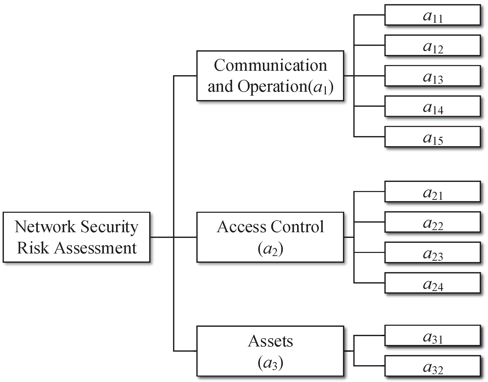
The index system is a hierarchical structure model, which divides the factors related to network risk into three levels. The framework of the index system of network security risk assessment is shown in Figure 1. The first level of the index system is network security risk assessment, also called the target level. In the second level, there are three criteria, communication and operation, access control and assets, respectively, which are all divided into 2∼5 smaller criteria at the bottom level (see Table 1).
3.1.2. Use D-S Evidence Theory to Fuse Mass Functions
In this approach, the weights of evidence are taken into account when using D-S evidence theory to fuse mass functions.
Let the set of evidence be . The weight coefficient of evidence is , where and . Let and the relative weight vector . Then, the “ratio” of BPA can be determined as , where , .
Use the “ratio” to discount BPA. The BPA after adjustment is:
Suppose the risk rank of the network is divided as . Ascertain all layer’s weights and BPA of the bottom layer with regard to , where represents the uncertainty. Use Equation (15) to adjust BPA, and then, use Equations (7) and (8) to combine evidence from bottom to top. Finally, BPA of the network risk can be obtained (). Note that BPA of middle level criteria still needs to be adjusted before being combined.
3.1.3. Obtain the Network Security Risk Value
After getting , the belief function of network risk can be obtained by Equation (5). At last, the network security risk value can be obtained through the risk calculation formula:
where represents the damage degree once the risk events happen. represents the average value of damage degree corresponding to the risk rank . Its range is .
3.1.4. Discussion of the Work Done by Gao et al.
In the approach proposed by Gao et al., the uncertainty of BPA is measured by the probability mass assigned to the complete set, which is not a very effective quantification of uncertainty. Moreover, only the subjective weights of criteria have been considered, which makes the subjectivity of the assessment very large. Therefore, in the novel assessment approach proposed in this paper, we employ an uncertainty measure to more accurately quantify the uncertainty of BPA and transform the uncertainty into objective weights. In addition, the weighted average combination method of combining mass functions, which has a good performance of convergence, is applied to the risk assessment. The process of the novel network security risk assessment approach is shown as below.
3.2. The Novel Network Security Risk Assessment Approach Proposed in This Paper
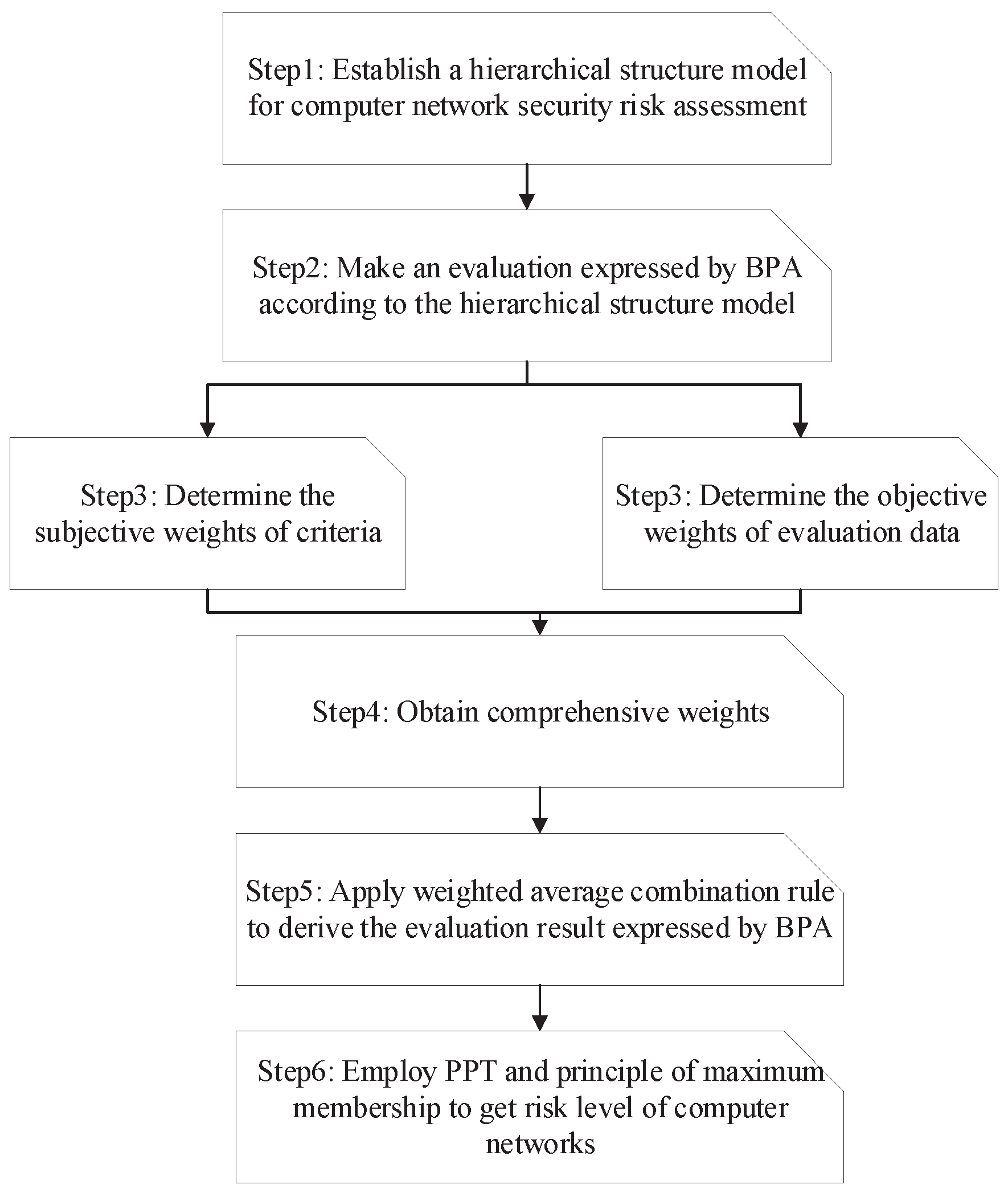
The purpose of this paper is to propose a better approach of network security risk assessment. The process of the novel network security risk assessment approach can be divided into six steps, as depicted in Figure 2.
3.2.1. Establish a Hierarchical Structure Model
3.2.2. Make an Evaluation Expressed by BPA
According to the hierarchical structure of computer network security risk assessment, the evaluation of the network, specifically the risk values of bottom criteria, should be given by experts and be expressed by BPA.
3.2.3. Determine the Subjective and Objective Weights
Assume that the subjective weights of the criteria are given by experts, which are known in advance. The objective weights are determined by the uncertainty of the evaluation data. The calculation method is as follows.
Let = {very low (VL), low (L), middle low (ML), middle (M), middle high (MH), high (H), very high (VH)} represent seven risk levels of network security assessment. For the bottom criteria, suppose the subjective weight and BPA of the criteria are and , respectively (). By using Equation (13), the uncertainty of each piece of evidence (evaluation data), denoted as (), can be calculated. In view of the larger uncertainty of evidence and the less useful information provided, the objective weight can be obtained by:
3.2.4. Obtain Comprehensive Weights
In this part, subjective weights of criteria and objective weights of evaluation data are combined to obtain the comprehensive weights. That is to say, the final weights of bottom criteria consist of two parts: the subjective weights known in advance and the objective weights to consider the uncertainty of mass functions, which contributes to decreasing the negative influence of expert’s extreme subjectivity on the evaluation data. The comprehensive weights are indicated by:
3.2.5. Use Weighted Average Combination Rule to Combine Mass Functions
Based on the comprehensive weights and BPAs () of the bottom criteria, the weighted average combination rule is used to combine the evidence in this layer. When the combination of evidence is finished, the results of the combination will be regarded as the mass functions (BPAs) of the middle level criteria. Similarly, we can calculate the comprehensive weights of criteria in this layer and combine the evidence to obtain the evaluation result, which is expressed by BPA. Besides, the uncertainty of the evaluation result can also be quantified by Equation (13).
3.2.6. Obtain the Risk Level of Computer Networks
Through above five steps, the BPA of network security risk assessment can be obtained. In this paper, by Equation (14), PPT is employed to convert the mass function into a probability distribution. Then, according to the principle of maximum membership, the risk level of computer networks is finally derived.
4. Case Studies
4.1. An Example of Network Security Risk Assessment
In this subsection, a numerical example from [25] is presented to illustrate the procedure of the proposed approach of evaluating network security.
4.1.1. Establish the Hierarchical Structure of Computer Networks
4.1.2. Make an Evaluation Expressed by BPA
4.1.3. Determine the Subjective and Objective Weights
4.1.4. Obtain Comprehensive Weights
4.1.5. Use Weighted Average Combination Rule to Combine the Mass Functions
On the basis of BPAs () of bottom criteria, along with the comprehensive weights , the weighed average of evidence can be calculated by Equation (9). Then, we can use Equations (7) and (8) to combine the weighted average of evidence 4 times to obtain . Similarly, we can derive and . Weighted average of evidence and the BPAs of the bottom criteria after combination are detailed in Table 6 and Table 7.
The BPAs of bottom criteria after combination can be viewed as the mass functions of middle level criteria. Similarly, the objective and comprehensive weights of these pieces of evidence can also be obtained (see Table 8). Then, the weighted average of evidence is derived. After using Equations (7) and (8) to combine 2 times, the combination result, denoted as m, which is also the mass function of network security risk assessment (see Table 9), is obtained. Meanwhile, the uncertainty of the evaluation result can be calculated by Equation (13), which is 0.0630 (quite small).
4.1.6. Obtain the Risk Level of Computer Networks
Through the last five steps, the evaluation result, which is expressed by BPA, is given. Applying PPT to the evaluation, the risk level of computer networks can be determined. The probability distribution after PPT is detailed in Table 10. According to the principle of maximum membership, the risk level of this computer network is middle high (MH).
Besides, the approach used in the study of [25] is also applied to compare with the approach proposed in this paper. As described in Figure 3, if the maximum membership principle is used to determine the risk level in these two approaches, they give the same assessment result, middle high. However, the approach proposed in this paper has a better performance of convergence, and the degree of evidence’s support for middle high (MH) is greater. More importantly, the uncertainty of the evaluation result in the study of [25] can be obtained by Equation (13), which is 0.1336, far greater than that of this paper.
Herein, we also compare and discuss the assessment of each middle level criterion by using these two assessment approach. The corresponding assessment results are shown in Table 7 and Table 11. Using the assessment approach proposed in this paper, the uncertainty of the evaluation results of , and can be obtained by using Equation (13), which is 0.1107, 0.1173 and 0.1450, respectively. In the approach proposed by Gao et al., the corresponding uncertainty is 0.1750, 0.1379 and 0.1953, respectively. Obviously, the use of our assessment approach can reduce the uncertainty of the assessment results. In addition, according to the evaluation data in Table 7, it can be seen that has the highest risk level, high (H). Therefore, more attention should be paid to to improve the overall network security.
All the above illustrates that the approach proposed in this paper can effectively assess the security of computer networks, which is the purpose of our study.
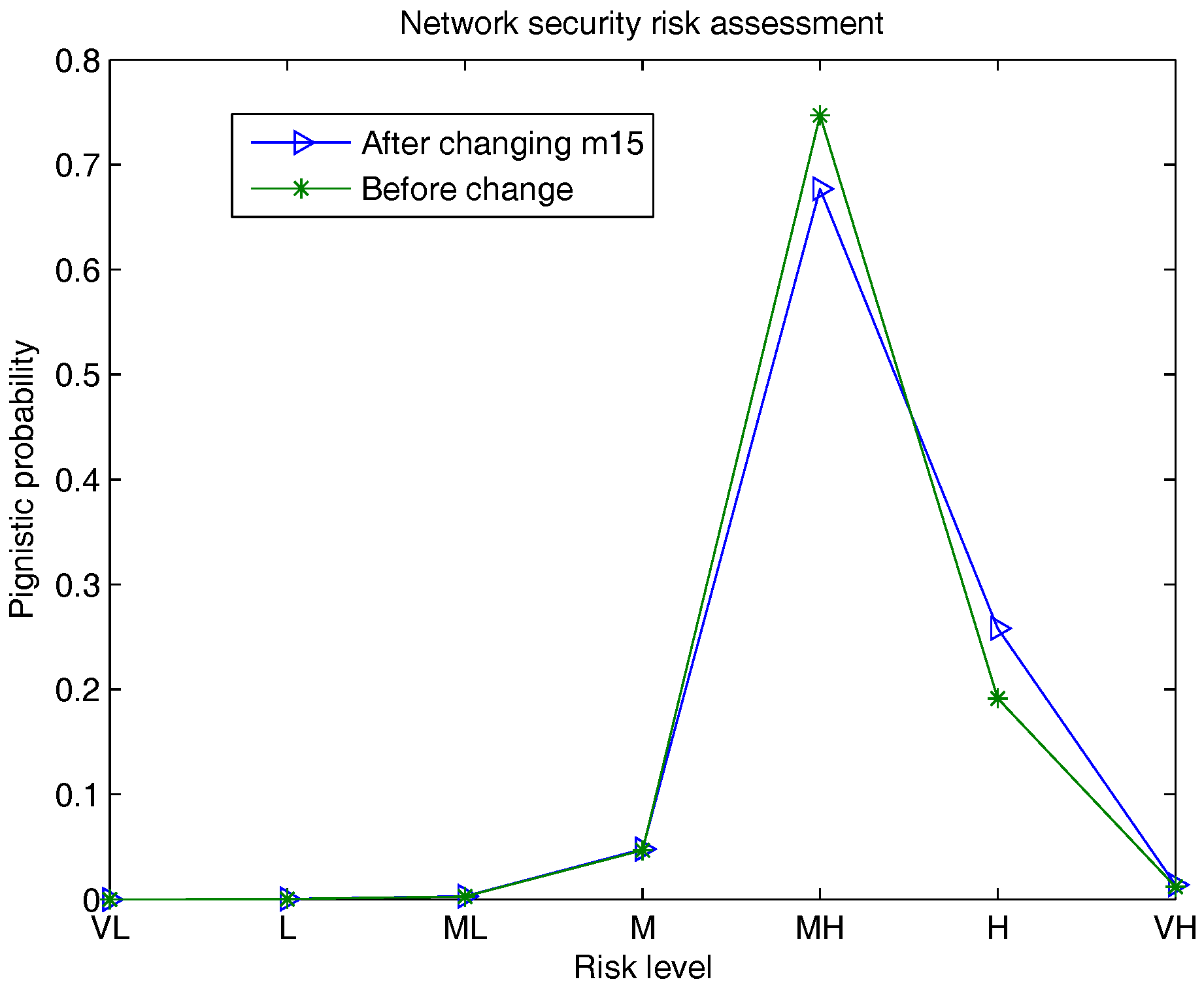
4.1.7. The Analysis of the Sensitivity of the Proposed Method
In this part, to examine the robustness of the proposed approach, the sensitivity analysis of the proposed approach is done by changing the BPAs of some criteria.
For example, the evidence of and (abbreviated as and ) is changed, respectively, by assigning all the probability mass to the complete set , which means maximizing the uncertainty and minimizing the useful information content. Then the evaluation result is calculated. The corresponding results are shown in Figure 4 and Figure 5.
From Figure 4 and Figure 5, it can be seen that although the uncertainty of the evidence increases and the useful information content reduces, the approach proposed in this paper can still make the correct evaluation, which proves that the proposed assessment approach is robust. Besides, changes in the evidence of the criterion with the larger weight will have a greater influence on the assessment result, which accords with this fact.
4.2. Another Example of Network Security System Assessment
Herein, an example of assessing computer network security systems is presented. This assessment is implemented in [53] by using a model with two-tuple linguistic information. In this subsection, evaluation data expressed in linguistic information in [53] are converted into BPAs, and then, the novel assessment approach proposed in this paper is employed to assess network security systems.
4.2.1. Use the Assessment Approach Proposed in This Paper to Assess Network Security Systems
There are four alternative network security systems from different information technology companies, denoted as , for the military to select. The purpose of assessing these network security systems is to assist the decision-maker in making the best choice. The attributes used to evaluate these computer network security systems are denoted as . They are tactics, technology, economy, logistics and strategy, respectively, and their weight vector is . There are three decision-makers, denoted as , and their weight vector is . The linguistic term set S is defined as S = , = , = , = , = , = , = }. The four possible alternatives are to be evaluated using the linguistic term set S by the three decision-makers under the above five attributes, and construct the decision matrices as follows:
The method to convert the decision matrices into BPAs is as follows.
- According to the weights of three decision-makers, the evaluation data based on linguistic information are transformed into the probability distribution of linguistic variables.
- By applying the uncertainty measure , the uncertainty of the probability distribution obtained in the previous step can be derived. Then, the uncertainty is used to discount the probability distribution to generate BPAs for evaluation.
The following gives an example to clearly illustrate the process of generating BPA for evaluation.
According to the decision matrices, for , the assessment of its desirability level under given by three decision-makers is , and , respectively. Then, the probability distribution of under is defined as:
By using Equation (13), the uncertainty of the probability distribution can be calculated as 0.1091. Let . Then, the final BPA for evaluation is defined as:
Using the same method, the BPAs of under attributes are calculated, as shown in Table 12, Table 13, Table 14 and Table 15. After getting the BPAs for evaluation, the novel assessment approach proposed in this paper is applied to assess the desirability level of network security systems. For each network security system, the subjective weights of attributes are known, which is . By using Equations (13) and (17), the corresponding objective weights are derived. Then, the comprehensive weights of attributes are calculated by Equation (18) (see Table 16). Using the weighted average combination rule to combine the BPAs of these five attributes, the evaluation results of network security systems are obtained (expressed by BPA), as shown in Table 17.
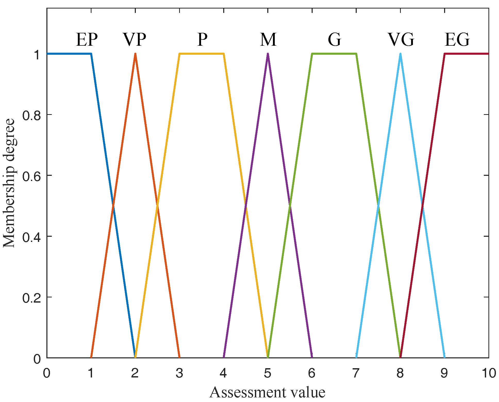
In order to rank these four network security systems, defuzzification is performed to get the total score for each network security system in this example. Suppose in the linguistic term set , every linguistic variable is represented by a trapezoidal fuzzy number given in Table 18 and graphically presented as Figure 6. The centroid defuzzification approach is used, and the defuzzified values for each linguistic variable are .
After obtaining the evaluation results of network security systems expressed by BPA, PPT is carried out. In this example, since the probability mass of BPA is all assigned to singleton sets, . Then, the total scores for these network security systems can be obtained by Equation (19), which are 8.6818, 2.6929, 5.0611, 7.2044, respectively. Therefore, the desirability level of these four network security systems is ranked as , and the most desirable alternative is , which is consistent with results given in [53]. That is to say, the novel assessment approach proposed in this paper is effective and can be applied to decision-making.
4.2.2. The Assessment of Network Security Systems by Using the Approach Proposed by Gao et al.
In this part, the assessment approach proposed in [25] is also employed to assess network security systems. The evaluation results (expressed by BPA) and the total scores of network security systems are shown in Table 19. From the total scores given by the assessment approach proposed in [25], the desirability level of these four network security systems is ranked as , which is also consistent with the results given in [53].
However, for , and , our novel assessment approach gives less uncertainty in the assessment results (BPA) than that of the assessment approach proposed in [25]. By using our approach, the uncertainty of the evaluation results (expressed by BPA) of , and can be obtained by Equation (13), which is 0.0698, 0.0478 and 0.0939, respectively; while the corresponding uncertainty by using the approach proposed by Gao et al. is 0.1001, 0.0949 and 0.1195, respectively.
For , these two assessment approaches give large differences in the assessment results (see Table 17 and Table 19). In our approach, the comprehensive weights used for evaluation are the combination of subjective weights and objective weights. It can be seen from Table 16 that after considering the uncertainty of each BPA and transforming it into objective weights, the comprehensive weights of attributes ∼ of have undergone significant changes. Among them, the weights of and are significantly increased, while the weights of and are significantly reduced, which leads to the larger probability mass assigned to and . That is to say, in our assessment approach, the uncertainty of the evaluation data makes the evaluation results more reasonable by adjusting the comprehensive weights. Therefore, it is more reasonable to assess by using the approach proposed in this paper.
4.2.3. The Ranking of Network Security Systems When Weights of Attributes Change
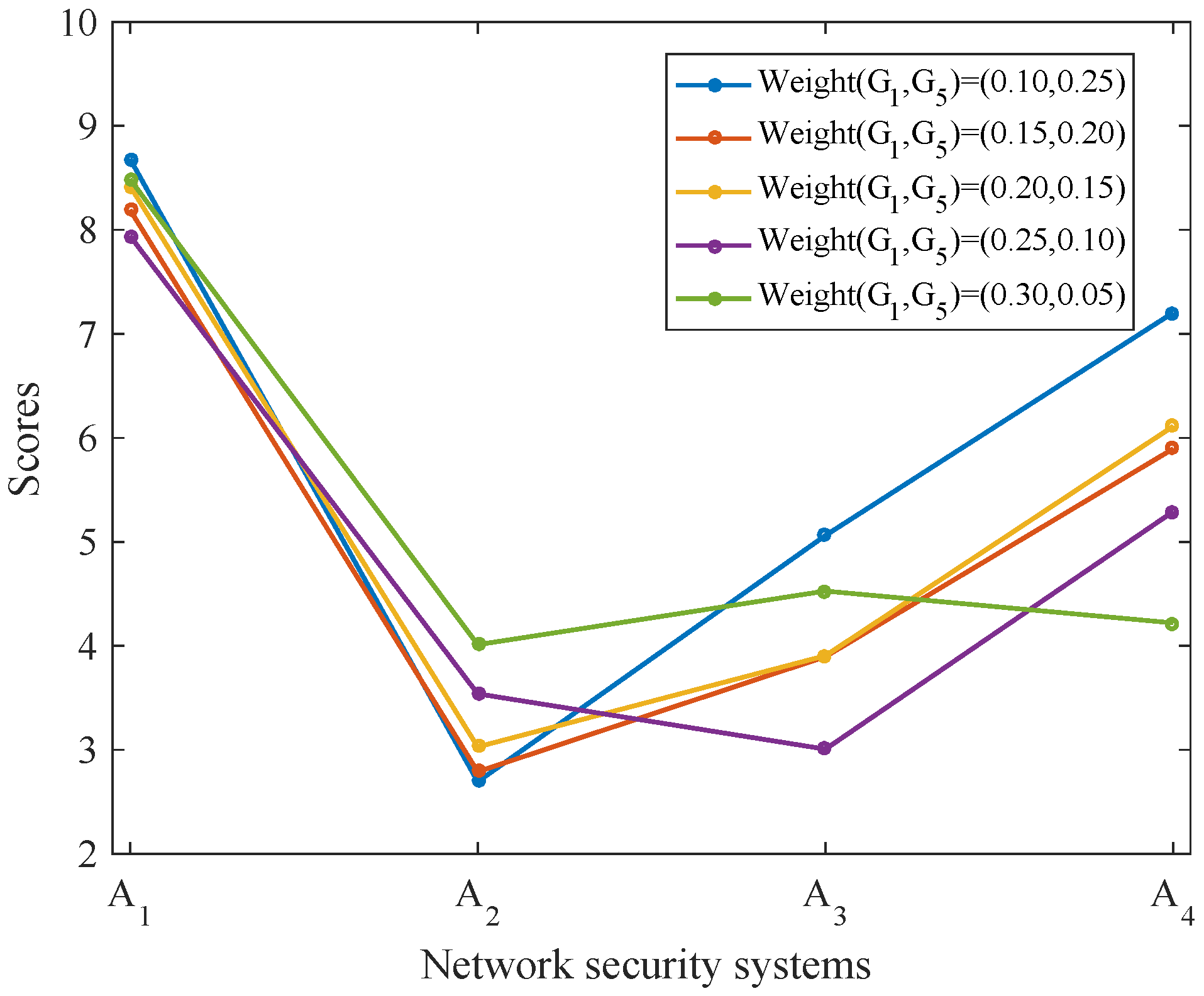
Herein, increase the weight (subjective weights) of , and reduce that of , while the weights of other attributes are unchanged, to observe the changes of the evaluation results of the network security system. The corresponding evaluation results are shown in Table 20 and Figure 7.
- The score of fluctuates at eight points and always ranks first, indicating that is excellent in both and .
- When the weights of and are changed, the score of decreases obviously. When , ranks third, with a very low score, indicating that is worse in and that more attention should be paid to .
- Similarly, the score of also decreases with the change of the weights of and , which indicates that there is a larger gap between and under than that under .
- The score of becomes higher and higher, indicating that more efforts should be made in to improve the overall situation of the network security system.
5. Conclusions
The contribution of this paper is to propose an effective approach of network security risk assessment. One of the crucial problems in the network security risk assessment is how to deal with uncertainty. In this paper, based on the hierarchical structure of network security risk assessment, an uncertainty measure is applied to quantify the uncertainty of the BPAs of criteria to obtain objective weights, and then, the comprehensive weights are obtained. Besides, the weighted average combination rule is adopted to combine the evidence from bottom to top. According to the probability distribution after using PPT and the principle of maximum membership, the risk level of computer networks can be determined.
Through analyzing the uncertainty of the evaluation results in the two illustrative examples, it is easy to find that the assessment approach proposed in this paper can significantly reduce the uncertainty of the evaluation result and give a clear and correct assessment. In addition, the second example also illustrates that our risk assessment approach of combining subjective and objective weights can be used in the decision-making field. Therefore, the novel risk assessment approach proposed in this paper is a very effective approach for assessing network security and for decision-making.
Acknowledgments
The authors are grateful to the anonymous reviewers for their useful comments and suggestions, which improved this paper. The work was partially supported by the National Natural Science Foundation of China (Program Nos. 61703338, 61671384), the Natural Science Basic Research Plan in Shaanxi Province of China (Program No. 2016JM6018), the Project of Science and Technology Foundation, Fundamental Research Funds for the Central Universities (Program No. 3102017OQD020) and the National Training Program of Innovation and Entrepreneurship for Undergraduates (Program No. 201710699190).
Author Contributions
Xinyang Deng and Yancui Duan proposed the idea of this paper. Yancui Duan, Yonghua Cai and Zhikang Wan calculated and analyzed the experimental data, where Yonghua Cai was responsible for programming. Yancui Duan wrote the paper. Xinyang Deng, Yonghua Cai and Zhikang Wan revised and improved the paper.
Conflicts of Interest
The authors declare no conflict of interest.
References
- Monostori, L.; Kádár, B.; Bauernhansl, T.; Kondoh, S.; Kumara, S.; Reinhart, G.; Sauer, O.; Schuh, G.; Sihn, W.; Ueda, K. Cyber-physical systems in manufacturing. CIRP Ann. Manuf. Technol. 2016, 65, 621–641. [Google Scholar] [CrossRef]
- Sridhar, S.; Hahn, A.; Govindarasu, M. Cyber–physical system security for the electric power grid. Proc. IEEE 2012, 100, 210–224. [Google Scholar]
- Shei, S.; Kalloniatis, C.; Mouratidis, H.; Delaney, A. Modelling secure cloud computing systems from a security requirements perspective. In Proceedings of the International Conference on Trust & Privacy in Digital Business, Porto, Portugal, 07–08 September 2016; pp. 48–62. [Google Scholar]
- Patel, S.C.; Bhatt, G.D.; Graham, J.H. Improving the cyber security of SCADA communication networks. Commun. ACM 2009, 52, 139–142. [Google Scholar] [CrossRef]
- Mavropoulos, O.; Mouratidis, H.; Fish, A.; Panaousis, E.; Kalloniatis, C. A conceptual model to support security analysis in the internet of things. Comput. Sci. Inf. Syst. 2017, 14, 557–578. [Google Scholar] [CrossRef]
- Scott-Hayward, S.; Natarajan, S.; Sezer, S. A survey of security in software defined networks. IEEE Commun. Surv. Tutor. 2016, 18, 623–654. [Google Scholar] [CrossRef]
- Butun, I.; Morgera, S.D.; Sankar, R. A survey of intrusion detection systems in wireless sensor networks. IEEE Commun. Surv. Tutor. 2014, 16, 266–282. [Google Scholar] [CrossRef]
- Langer, L.; Skopik, F.; Smith, P.; Kammerstetter, M. From old to new: Assessing cybersecurity risks for an evolving smart grid. Comput. Secur. 2016, 62, 165–176. [Google Scholar] [CrossRef]
- Zhang, Y.; Xiao, Y.; Ghaboosi, K.; Zhang, J.; Deng, H. A survey of cyber crimes. Secur. Commun. Netw. 2012, 5, 422–437. [Google Scholar] [CrossRef]
- Sharma, P.; Doshi, D.; Prajapati, M.M. Cybercrime: Internal security threat. In Proceedings of the IEEE International Conference on ICT in Business Industry & Government (ICTBIG), Indore, India, 18–19 November 2016; pp. 1–4. [Google Scholar]
- Yang, P. Study on cyber crime investigation and forensics based on internet traceability of computer firewall protocol. In Frontiers of Manufacturing Science & Measuring Technology V; C Book News: Portland, OR, USA, 2015; pp. 511–516. [Google Scholar]
- Gu, W.; Xu, L.; Ren, M.; Han, X. Network forensics scenario reconstruction method based on hidden Markov models. In Proceedings of the 2015 IEEE 7th International Conference on Information Technology in Medicine & Education (ITME), Huangshan, China, 13–15 November 2015; pp. 500–505. [Google Scholar]
- Li, Y.; Yan, J. Elf-based computer virus prevention technologies. In Information Computing & Applications, Pt II; National Natural Science Foundation of China (NSFC): Beijing, China, 2011; pp. 621–628. [Google Scholar]
- Zeng, L.; Xiao, Y.; Chen, H.; Sun, B.; Han, W. Computer operating system logging and security issues: A survey. Secur. Commun. Netw. 2016, 9, 4804–4821. [Google Scholar] [CrossRef]
- Kamarudin, M.H.; Maple, C.; Watson, T.; Safa, N.S. A logitboost-based algorithm for detecting known and unknown web attacks. IEEE Access 2017, 5, 26190–26200. [Google Scholar] [CrossRef]
- Liang, X.; Xiao, Y. Game theory for network security. IEEE Commun. Surv. Tutor. 2013, 15, 472–486. [Google Scholar] [CrossRef]
- Zheng, Z.; Sun, P. Application of RBF neural network in network security risk assessment. In Proceedings of the 2011 International Conference On Computational Science & Applications, Antwerp, Belgium, 26–27 March 2011; pp. 43–46. [Google Scholar]
- Kotenko, I.; Doynikova, E. Security assessment of computer networks based on attack graphs and security events. In Proceedings of the Information & Communication Technology-EurAsia Conference, Bali, Indonesia, 14–17 April 2014; pp. 462–471. [Google Scholar]
- Liang, L.; Yang, J.; Liu, G.; Zhu, G.; Yang, Y. Novel method of assessing network security risks based on vulnerability correlation graph. In Proceedings of the 2012 IEEE 2nd International Conference on Computer Science & Network Technology (ICCSNT), Changchun, China, 29–31 December 2012; pp. 1085–1090. [Google Scholar]
- Munir, R.; Disso, J.P.; Awan, I.; Mufti, M.R. A quantitative measure of the security risk level of enterprise networks. In Proceedings of the 2013 IEEE 8th International Conference on Broadband & Wireless Computing, Communication & Applications (BWCCA), Compiegne, France, 28–30 October 2013; pp. 437–442. [Google Scholar]
- Fei, J.; Xu, H. Assessing computer network security with fuzzy analytic hierarchy process. In Proceedings of the 2010 IEEE 2nd International Conference on Advanced Computer Control (ICACC), Shenyang, China, 27–29 March 2010; pp. 204–208. [Google Scholar]
- Li, C. Research on computer network security assessment based on fuzzy analytic hierarchy process. In Proceedings of the 2016 4th International Conference On Machinery, Materials & Computing Technology, Hangzhou, China, 23–24 January 2016; pp. 110–115. [Google Scholar]
- Dongmei, Q.; Chunshu, F. Study on network security assessment based on analytical hierarchy process. In Proceedings of the 2011 IEEE International Conference On Electronics, Communications & Control (ICECC), Ningbo, China, 9–11 September 2011; pp. 2320–2323. [Google Scholar]
- Feng, N.; Li, M. An information systems security risk assessment model under uncertain environment. Appl. Soft Comput. 2011, 11, 4332–4340. [Google Scholar] [CrossRef]
- Gao, H.; Zhu, J.; Li, C. The analysis of uncertainty of network security risk assessment using Dempster–Shafer theory. In Proceedings of the 2008 IEEE 12th International Conference On Computer Supported Cooperative Work In Design (CSCWD), Xi’an, China, 16–18 April 2008; pp. 754–759. [Google Scholar]
- Zedeh, L. Fuzzy sets. Information & Control 1965, 8, 338–353. [Google Scholar]
- Jiang, W.; Wei, B.; Liu, X.; Li, X.; Zheng, H. Intuitionistic fuzzy power aggregation operator based on entropy and its application in decision making. Int. J. Intell. Syst. 2018, 33, 49–67. [Google Scholar] [CrossRef]
- Jiang, W.; Wei, B. Intuitionistic fuzzy evidential power aggregation operator and its application in multiple criteria decision-making. Int. J. Syst. Sci. 2018, 49, 582–594. [Google Scholar] [CrossRef]
- Pawlak, Z. Rough sets. Int. J. Parallel Program. 1982, 11, 341–356. [Google Scholar] [CrossRef]
- Dubois, D.; Prade, H. Possibility Theory: An Approach to Computerized Processing of Uncertainty; Plenum Press: New York, NY, USA, 1988. [Google Scholar]
- Dempster, A.P. Upper and lower probabilities induced by a multivalued mapping. Ann. Math. Stat. 1967, 38, 325–339. [Google Scholar] [CrossRef]
- Shafer, G. A Mathematical Theory of Evidence; Princeton University Press: Princeton, NJ, USA, 1976. [Google Scholar]
- Deng, Y. Generalized evidence theory. Appl. Intell. 2015, 43, 530–543. [Google Scholar] [CrossRef]
- Jiang, W.; Zhan, J. A modified combination rule in generalized evidence theory. Appl. Intell. 2017, 46, 630–640. [Google Scholar] [CrossRef]
- Deng, X.; Xiao, F.; Deng, Y. An improved distance-based total uncertainty measure in belief function theory. Appl. Intell. 2017, 46, 898–915. [Google Scholar] [CrossRef]
- Deng, Y.; Shi, W.; Zhu, Z.; Liu, Q. Combining belief functions based on distance of evidence. Decis. Support Syst. 2004, 38, 489–493. [Google Scholar]
- Jiang, W.; Chang, Y.; Wang, S. A method to identify the incomplete framework of discernment in evidence theory. Math. Prob. Eng. 2017, 2017, 7635972. [Google Scholar] [CrossRef]
- Deng, X.; Jiang, W. An evidential axiomatic design approach for decision making using the evaluation of belief structure satisfaction to uncertain target values. Int. J. Intell. Syst. 2018, 33, 15–32. [Google Scholar] [CrossRef]
- Deng, X.; Deng, Y. D-AHP method with different credibility of information. Soft Comput. 2018. [Google Scholar] [CrossRef]
- Jiang, W.; Xie, C.; Zhuang, M.; Tang, Y. Failure mode and effects analysis based on a novel fuzzy evidential method. Appl. Soft Comput. 2017, 57, 672–683. [Google Scholar] [CrossRef]
- Zheng, X.; Deng, Y. Dependence assessment in human reliability analysis based on evidence credibility decay model and IOWA operator. Ann. Nuclear Energy 2018, 112, 673–684. [Google Scholar] [CrossRef]
- Xu, H.; Deng, Y. Dependent evidence combination based on Shearman coefficient and Pearson coefficient. IEEE Access 2018. [Google Scholar] [CrossRef]
- Deng, X.; Han, D.; Dezert, J.; Deng, Y.; Shyr, Y. Evidence combination from an evolutionary game theory perspective. IEEE Trans. Cybern. 2016, 46, 2070–2082. [Google Scholar] [CrossRef] [PubMed]
- Yu, C.; Yang, J.; Yang, D.; Ma, X.; Min, H. An improved conflicting evidence combination approach based on a new supporting probability distance. Expert Syst. Appl. 2015, 42, 5139–5149. [Google Scholar] [CrossRef]
- Murphy, C.K. Combining belief functions when evidence conflicts. Decis. Support Syst. 2000, 29, 1–9. [Google Scholar] [CrossRef]
- Deng, Y. Deng entropy. Chaos Solitons Fractals 2016, 91, 549–553. [Google Scholar] [CrossRef]
- Harmanec, D.; Klir, G.J. Measuring total uncertainty in Dempster–Shafer theory: A novel approach. Int. J. Gen. Syst. 1994, 22, 405–419. [Google Scholar] [CrossRef]
- Jousselme, A.L.; Liu, C.; Grenier, D.; Bossé, É. Measuring ambiguity in the evidence theory. IEEE Trans. Syst. Man Cybern. Part A Syst. Hum. 2006, 36, 890–903. [Google Scholar] [CrossRef]
- Jiang, W.; Wang, S. An uncertainty measure for interval-valued evidences. Int. J. Comput. Commun. Control 2017, 12, 631–644. [Google Scholar] [CrossRef]
- Wang, X.; Song, Y. Uncertainty measure in evidence theory with its applications. Appl. Intell. 2017. [Google Scholar] [CrossRef]
- Yang, Y.; Han, D. A new distance-based total uncertainty measure in the theory of belief functions. Knowl. Based Syst. 2016, 94, 114–123. [Google Scholar] [CrossRef]
- Smets, P.; Kennes, R. The transferable belief model. Artif. Intell. 1994, 66, 191–234. [Google Scholar] [CrossRef]
- Zhang, S. A model for evaluating computer network security systems with 2-tuple linguistic information. Comput. Math. Appl. 2011, 62, 1916–1922. [Google Scholar] [CrossRef]
Figure 1.
The hierarchical structure model [25].
Figure 1.
The hierarchical structure model [25].

Figure 2.
Development of the proposed method.

Figure 3.
Comparison of evaluation results of different methods.
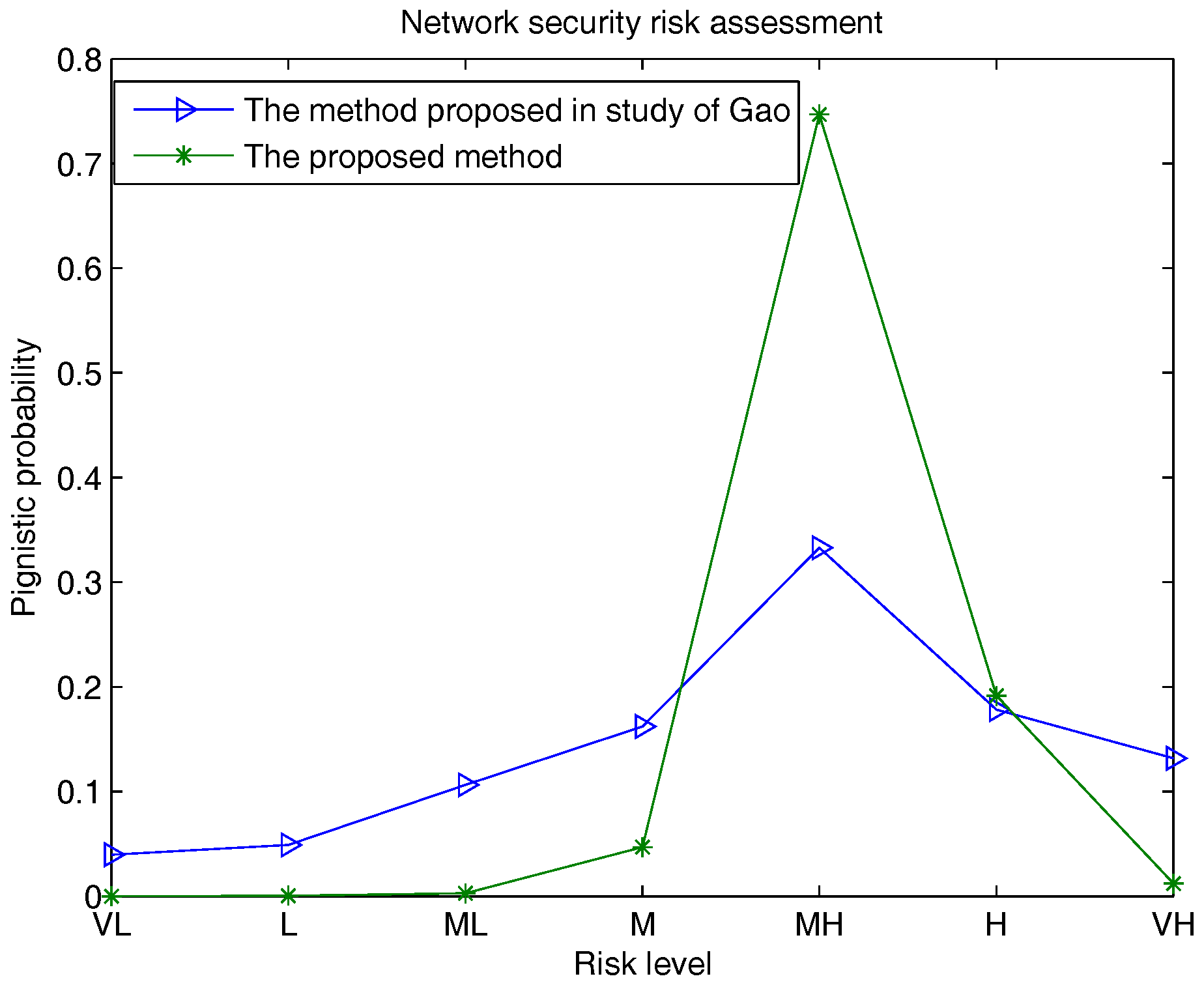
Figure 4.
Comparison of evaluation results before and after changing .

Figure 5.
Comparison of evaluation results before and after changing evidence .
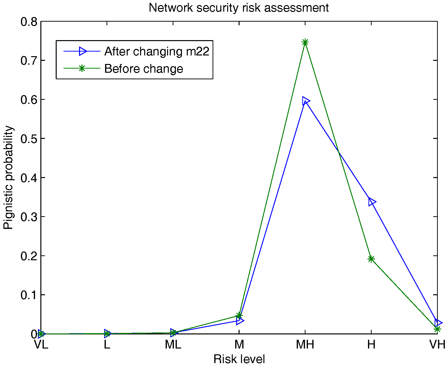
Figure 6.
The geometric representation of linguistic variables in Table 18 including extremely poor (EP), very poor (VP), poor (P), medium (M), good (G), very good (VG), extremely good (EG).
Figure 6.
The geometric representation of linguistic variables in Table 18 including extremely poor (EP), very poor (VP), poor (P), medium (M), good (G), very good (VG), extremely good (EG).

Figure 7.
The ranking of the network security system.

Table 1.
Criteria of the bottom level [25].
Table 1.
Criteria of the bottom level [25].
| Criteria | Description of the Criteria |
|---|---|
| Prevention of Malice Software | |
| Media Processing and Security | |
| Operation Program and Duty | |
| Network Management | |
| Information and Software, Hardware Exchange | |
| Management of Network Access | |
| Management of User’s Access | |
| Management of Application Access | |
| System Access and Monitoring of Usage | |
| Effect on Tangible Assets | |
| Effect on Intangible Assets |
Table 2.
The basic probability assignments (BPAs) of bottom criteria [25]: very low (VL), low (L), middle low (ML), middle (M), middle high (MH), high (H), very high (VH).
Table 2.
The basic probability assignments (BPAs) of bottom criteria [25]: very low (VL), low (L), middle low (ML), middle (M), middle high (MH), high (H), very high (VH).
| Bottom Criteria | BPA | |||||||
|---|---|---|---|---|---|---|---|---|
| VL | L | ML | M | MH | H | VH | ||
| 0 | 0.1 | 0.1 | 0.2 | 0.2 | 0.3 | 0.1 | 0 | |
| 0 | 0.1 | 0.1 | 0.2 | 0.2 | 0.2 | 0.1 | 0.1 | |
| 0 | 0.1 | 0.15 | 0.2 | 0.3 | 0.15 | 0 | 0.1 | |
| 0 | 0.1 | 0.1 | 0.15 | 0.2 | 0.3 | 0.1 | 0.05 | |
| 0.1 | 0.1 | 0.1 | 0.2 | 0.3 | 0.1 | 0 | 0.1 | |
| 0 | 0 | 0.1 | 0.1 | 0.2 | 0.2 | 0.3 | 0.1 | |
| 0.1 | 0.1 | 0.15 | 0.2 | 0.2 | 0.1 | 0.1 | 0.05 | |
| 0.1 | 0.1 | 0.1 | 0.1 | 0.2 | 0.2 | 0.1 | 0.1 | |
| 0 | 0.1 | 0.1 | 0.2 | 0.3 | 0.2 | 0.1 | 0 | |
| 0 | 0.1 | 0.1 | 0.1 | 0.3 | 0.2 | 0.1 | 0.1 | |
| 0 | 0 | 0.1 | 0.1 | 0.2 | 0.2 | 0.3 | 0.1 | |
Table 3.
Subjective weights of criteria.
| Middle Level Criteria | Subjective Weights | Bottom Criteria | Subjective Weights |
|---|---|---|---|
| 0.310 | 0.157 | ||
| 0.393 | |||
| 0.164 | |||
| 0.172 | |||
| 0.114 | |||
| 0.580 | 0.281 | ||
| 0.312 | |||
| 0.280 | |||
| 0.127 | |||
| 0.110 | 0.670 | ||
| 0.330 |
Table 4.
Objective weights of bottom criteria.
| Bottom Criteria | Uncertainty Values | Objective Weights |
|---|---|---|
| 0.1247 | 0.2847 | |
| 0.2139 | 0.1660 | |
| 0.2093 | 0.1697 | |
| 0.1681 | 0.2112 | |
| 0.2109 | 0.1684 | |
| 0.2087 | 0.2063 | |
| 0.1729 | 0.2491 | |
| 0.2161 | 0.1993 | |
| 0.1247 | 0.3453 | |
| 0.2109 | 0.4974 | |
| 0.2087 | 0.5026 |
Table 5.
Comprehensive weights of bottom criteria.
| Bottom Criteria | Subjective Weights | Objective Weights | Comprehensive Weights |
|---|---|---|---|
| 0.1570 | 0.2847 | 0.2312 | |
| 0.3930 | 0.1660 | 0.3375 | |
| 0.1640 | 0.1697 | 0.1440 | |
| 0.1720 | 0.2112 | 0.1879 | |
| 0.1140 | 0.1684 | 0.0993 | |
| 0.2810 | 0.2063 | 0.2463 | |
| 0.3120 | 0.2491 | 0.3302 | |
| 0.2800 | 0.1993 | 0.2371 | |
| 0.1270 | 0.3453 | 0.1863 | |
| 0.6700 | 0.4974 | 0.6677 | |
| 0.3300 | 0.5026 | 0.3323 |
Table 6.
The weighted average of evidence of bottom criteria.
| VL | L | ML | M | MH | H | VH | ||
|---|---|---|---|---|---|---|---|---|
| 0.0099 | 0.1000 | 0.1072 | 0.1906 | 0.2243 | 0.2248 | 0.0757 | 0.0675 | |
| 0.0567 | 0.0754 | 0.1165 | 0.1517 | 0.2186 | 0.1670 | 0.1493 | 0.0649 | |
| 0 | 0.0668 | 0.1000 | 0.1000 | 0.2668 | 0.2000 | 0.1665 | 0.1000 |
Table 7.
The BPAs of bottom criteria after combination.
| VL | L | ML | M | MH | H | VH | ||
|---|---|---|---|---|---|---|---|---|
| 0.0002 | 0.0227 | 0.0281 | 0.1991 | 0.3682 | 0.3713 | 0.0102 | 0.0002 | |
| 0.0132 | 0.0242 | 0.0699 | 0.1431 | 0.4230 | 0.1885 | 0.1369 | 0.0012 | |
| 0 | 0.0504 | 0.0849 | 0.0849 | 0.3524 | 0.2264 | 0.1727 | 0.0283 |
Table 8.
Objective and comprehensive weights of middle level criteria.
| Middle Level Criteria | Subjective Weights | Objective Weights | Comprehensive Weights |
|---|---|---|---|
| 0.31 | 0.3692 | 0.3291 | |
| 0.58 | 0.3487 | 0.5816 | |
| 0.11 | 0.2821 | 0.0892 |
Table 9.
The weighted average evidence and combination result of middle level criteria.
| VL | L | ML | M | MH | H | VH | ||
|---|---|---|---|---|---|---|---|---|
| 0.0077 | 0.0261 | 0.0575 | 0.1564 | 0.3986 | 0.2521 | 0.0984 | 0.0033 | |
| m | 0 | 0.0003 | 0.0026 | 0.0468 | 0.7468 | 0.1915 | 0.0121 | 0 |
Table 10.
The probability distribution of the evaluation result.
| VL | L | ML | M | MH | H | VH | |
|---|---|---|---|---|---|---|---|
| 0 | 0.0003 | 0.0026 | 0.0468 | 0.7468 | 0.1915 | 0.0121 |
Table 11.
The BPAs of bottom criteria after combination in [25].
Table 11.
The BPAs of bottom criteria after combination in [25].
| VL | L | ML | M | MH | H | VH | ||
|---|---|---|---|---|---|---|---|---|
| 0.0023 | 0.0886 | 0.0932 | 0.2082 | 0.2439 | 0.2321 | 0.0743 | 0.0575 | |
| 0.0474 | 0.0516 | 0.1151 | 0.1577 | 0.3033 | 0.1656 | 0.1452 | 0.014 | |
| 0 | 0.0825 | 0.0971 | 0.0971 | 0.3058 | 0.2088 | 0.1263 | 0.0825 |
Table 12.
BPAs of the attributes of .
| Attributes | BPA |
|---|---|
Table 13.
BPAs of the attributes of .
| Attributes | BPA |
|---|---|
Table 14.
BPAs of the attributes of .
| Attributes | BPA |
|---|---|
Table 15.
BPAs of the attributes of .
| Attributes | BPA |
|---|---|
Table 16.
The comprehensive weights of the attributes of .
| Network Security System | Comprehensive Weights of Attributes |
|---|---|
Table 17.
The evaluation results (expressed by BPA).
| Network Security System | The Evaluation Results (Expressed by BPA) |
|---|---|
Table 18.
Linguistic variables for the evaluation.
| Linguistic Variable | Fuzzy Numbers |
|---|---|
| (EP) | (0,0,1,2) |
| (VP) | (1,2,2,3) |
| (P) | (2,3,4,5) |
| (M) | (4,5,5,6) |
| (G) | (5,6,7,8) |
| (VG) | (7,8,8,9) |
| (GP) | (8,9,10,10) |
Table 19.
The evaluation results by using the assessment approach in [25].
Table 19.
The evaluation results by using the assessment approach in [25].
| Network Security System | The Total Score | BPA |
|---|---|---|
| 7.9622 | ||
| 3.1515 | ||
| 4.0068 | ||
| 6.2797 | ||
Table 20.
The ranking of the network security system.
| Weight () | Scores () | Ranking |
|---|---|---|
| (0.10,0.25) | (8.6818,2.6929,5.0611,7.2044) | |
| (0.15,0.20) | (8.1930,2.7884,3.8953,5.8952) | |
| (0.20,0.15) | (8.4226,3.0275,3.9050,6.1114) | |
| (0.25,0.10) | (7.9419,3.5380,3.0057,5.2914) | |
| (0.30,0.05) | (8.4870,4.0109,4.5264,4.2198) |
© 2018 by the authors. Licensee MDPI, Basel, Switzerland. This article is an open access article distributed under the terms and conditions of the Creative Commons Attribution (CC BY) license (http://creativecommons.org/licenses/by/4.0/).
Share and Cite
MDPI and ACS Style
Duan, Y.; Cai, Y.; Wang, Z.; Deng, X. A Novel Network Security Risk Assessment Approach by Combining Subjective and Objective Weights under Uncertainty. Appl. Sci. 2018, 8, 428. https://doi.org/10.3390/app8030428
AMA Style
Duan Y, Cai Y, Wang Z, Deng X. A Novel Network Security Risk Assessment Approach by Combining Subjective and Objective Weights under Uncertainty. Applied Sciences. 2018; 8(3):428. https://doi.org/10.3390/app8030428
Chicago/Turabian StyleDuan, Yancui, Yonghua Cai, Zhikang Wang, and Xinyang Deng. 2018. "A Novel Network Security Risk Assessment Approach by Combining Subjective and Objective Weights under Uncertainty" Applied Sciences 8, no. 3: 428. https://doi.org/10.3390/app8030428
Note that from the first issue of 2016, this journal uses article numbers instead of page numbers. See further details here.