Pressure Transient Model of Water-Hydraulic Pipelines with Cavitation

Abstract

Transient pressure investigation of water-hydraulic pipelines is a challenge in the fluid transmission field, since the flow continuity equation and momentum equation are partial differential, and the vaporous cavitation has high dynamics; the frictional force caused by fluid viscosity is especially uncertain. In this study, due to the different transient pressure dynamics in upstream and downstream pipelines, the finite difference method (FDM) is adopted to handle pressure transients with and without cavitation, as well as steady friction and frequency-dependent unsteady friction. Different from the traditional method of characteristics (MOC), the FDM is advantageous in terms of the simple and convenient computation. Furthermore, the mechanism of cavitation growth and collapse are captured both upstream and downstream of the water-hydraulic pipeline, i.e., the cavitation start time, the end time, the duration, the maximum volume, and the corresponding time points. By referring to the experimental results of two previous works, the comparative simulation results of two computation methods are verified in experimental water-hydraulic pipelines, which indicates that the finite difference method shows better data consistency than the MOC.

1. Introduction

Transient pressure pulsations generated by the rapid closure of a valve would easily cause hydraulic pipeline systems to burst because the pressure pulsations exceed the safe operating range of such pipelines. Violent pressure pulsations result in cavitation growth and collapse in these systems. To study the mechanism of cavitation during pressure transient pulsations, it is necessary to investigate the cavitation appearance, its volume evaluation, and the effect on the pipeline and hydraulic systems.

Pressure transients with cavitation in pipelines have been investigated by many researchers. Kojima et al. [1] presented the gas-nonbubbly flow model to predict pressure increments, which involved cavitation on the downstream side of the pipeline as a valve was instantaneously closed. They used a water–glycol mixture and an oil/water emulsion fluid including mineral oil as working fluids and compared the computed pressure pulsations with experimental results. Chaudhry et al. [2,3] then proposed a MacCormack scheme and a Gabutti scheme for pressure transient analysis, which was verified both in computed simulation and experimental studies. Although modeling accuracy was achieved, discrepancies in the pressure magnitudes between simulations and experiments were found. Transient pressure pulsations often lead to unexpected chatter, overshooting, and a zero bias of tracking error in the electrohydraulic control system [4,5,6,7]. Shu et al. [8,9,10] developed a vaporous cavitation model that used a two-phase homogeneous equilibrium to simulate pipeline pressure transients with upstream, midstream, and downstream cavitation. Bergant et al. [11,12] discussed three cavitation models: the discrete vapor cavity model (DVCM), the discrete gas cavity model (DGCM), and the generalized interface vaporous cavitation model (GIVCM). The comparative results of the three cavitation models indicated that the GIVCM was able to directly obtain the regions of vaporous cavitation occurrence. Jiang et al. [13,14,15,16], via genetic algorithms, developed the parametric identification of the gas bubble model and the frequency-dependent friction model. Parametric identification and noise suppression are also addressed in mechanical ventilation [17,18,19,20]. Sadafi et al. [21] recently studied water hammers with cavitation in a simple reservoir-pipeline-valve system and a pumping station. Karadžić et al. [22] verified the robustness of the DGCM via analysis of the experimental results. Iglesias-Rey et al. [23] performed a detailed study of the actual behavior of different valves (both air intake and exhaust) and described the mathematical characterization of different commercial valves. Fuertes-Miquel et al. [24] presented a numerical modeling of pipelines with air pockets and air valves to study the behavior of the air inside pipes as the air was expelled through air valves. Majd et al. [25] investigated the unsteady flow of a non-Newtonian fluid due to the instantaneous valve closure in a pipeline. Comparison revealed a remarkable deviation in pressure history and velocity profile with respect to the water hammer in Newtonian fluids. Zhou et al. [26] adopted a second-order finite volume method for cavitation in the water column separation of pipelines to capture vapor cavities and predict their growth and collapse. Wang et al. [27] adopted a two-dimensional CFD model to characterize liquid column separation. The simulation results revealed the formation of an intermediate cavity and both the location and shape of the region undergoing distributed vaporous cavitation. Himr [28] also studied water hammers with column separation as a one-dimensional flow. The volume of the cavity was determined by Gibson’s method, and the air bubbles were considered to affect the speed of sound.

Thanks to the research development of transient pressure in the fluid transmission field, the main contributions of this paper are as follows:

(i) Different from [10], a pressure transient model of water-hydraulic pipelines is constructed to reveal both the transient pressure magnitude and the dynamic characteristics of cavitation volume. To the authors’ best knowledge, there have been few attempts to predict cavitation volume changes and illustrate its influence on pressure transients in hydraulic pipelines, as described in [14,15]. Although the simplified cavitation model is based on a flow continuity principle [29], the frictional force in pipelines involving the steady friction force and the frequency-dependent unsteady friction should be a primary consideration in pressure transient analysis.

(ii) Different from the MOC, the FDM is adopted to estimate the magnitudes of the pressure peaks and the changes in cavitation volume to adapt the transient pressure both with and without cavitation. Simultaneously, the respective boundary conditions of both the upstream and downstream sides of the valve are also considered. A comparison with the MOC is made; results are verified by the percentage of the integral of the absolute difference (IAD) between simulation and experimental reference results.

2. Mathematical Models

2.1. Basic Equations without Cavitation

The simple water-hydraulic pipe is shown in Figure 1. To illustrate the propagation and reflection of the pressure transients, the sequence of events, which is caused by a valve closure in the middle of the pipe connected with the downstream and upstream tanks, will be discussed. Without a loss of generality, the pipe diameter is assumed to be constant, and the released gas is negligible.

The general model of pressure transients in the pipeline involves the continuity equation and the momentum equation, which are mentioned in Wylie et al. [29]. The continuity equation is derived from the mass conservation law as follows:

$$\frac{1}{c_0^2}\frac{\partial p}{\partial t}+\frac{\rho }{\pi r_0^2}\frac{\partial q}{\partial x}=0,$$

(1)

where p is the pressure in pipeline, q is the flow rate, $\rho$ is the density of fluid, $c_0$ is the acoustic velocity in the fluid, $r_0$ is the radius of the pipeline, x is the spatial variable, and t is the time variable.

Meanwhile, the equation of momentum is constructed by Newton’s law of motion as follows:

$$\frac{\rho }{\pi r_0^2}\frac{\partial q}{\partial t}+\frac{\partial p}{\partial x}+F\left(q\right)=0.$$

(2)

In Equation (1), $c_0$ can be given by

$$c_0=\sqrt{B_{eff}/\rho },$$

(3)

where $B_{eff}$ is the effective bulk modulus.

2.2. Continuity Equation under Vaporous Cavitation Condition

The cavitation normally arises when the pressure transients in pipelines are closed to the vapor pressure. If the pressure in the pipeline drops to or below the vapor pressure, vapor cavitation will form. Furthermore, if the pressure stays at the level of the vapor pressure and the cavitation size has approached a critical diameter, the cavitation will continue to grow rapidly. However, the cavitation will be unstable and collapse until the pressure is greater than the vapor pressure.

Pettersson et al. [30] and Harris et al. [31] presented a relatively simple cavitation model that illustrates the dynamic characteristics of piston pumps and can capture the key aspects of cavitation. Since the pressure in the pipeline element is assumed to be the vapor pressure under a vaporous cavitation condition, according to the flow continuity principle, the dynamics of the cavitation volume $V_{cav}$ is given by

$$\frac{d{V}_{cav}}{dt}=q_{out}-q_{in},$$

(4)

where $q_{out}$ and $q_{in}$ are the outflow rate and inflow rate of an element in the pipe, respectively.

2.3. Frictional Items

Due to the fluid viscosity, the frictional force $F\left(q\right)$ in Equation (2) can be described as the sum of the steady friction item and the frequency-dependent unsteady friction item. Zielke [32] considered the frequency-dependent friction item as some weighting functions described in the frequency domain via Laplace transform. Subsequently, Trikha [33] proposed three exponent function items to estimate the frequency-dependent friction. Then, Taylor et al. [34] optimized the coefficients of the Trikha model and proposed an approximate model with four exponent function items as follows:

$$F\left(q\right)=F_0+\frac{1}{2}\sum _{i=1}^4{Y}_i,$$

(5)

where the first item $F_0$ is the steady friction, and the second item is the frequency-dependent unsteady friction. Based on the Darcy–Weisbach equation, $F_0$ can be expressed as

$$F_0=\frac{\rho fv\left|v\right|}{4r_0}.$$

(6)

The four items of frequency-dependent friction $Y_i$ can be computed by

$$\left\{\begin{array}{c}\begin{array}{c}\frac{\partial Y_i}{\partial t}=-\frac{n_i\mu }{\rho r_0^2}{Y}_i+m_i\frac{\partial F_0}{\partial t}\hfill \\ Y_i\left(0\right)=0\hfill \end{array}\hfill \end{array}\right.,i=1,\dots ,4$$

(7)

where the constants $n_i$ and $m_i$ are listed in

Table 1. $n_i$ and $m_i$.

i	1	2	3	4
$n_i$	$3.9479\times {10}^1$	$2.9829\times {10}^2$	$2.2279\times {10}^3$	$8.8782\times {10}^4$
$m_i$	2.0141	5.3946	$1.6259\times {10}^1$	$3.2048\times {10}^2$

.

3. Simulation Methods

Two predictive methods, i.e., MOC and FDM, are presented. In order to solve the two partial differential equations in terms of pressure and flow rate, the pipeline is divided into n elements of equal length $\Delta x=L/n$, where L is the pipeline length. It should be noted that different test values of the pipeline length L can be selected in simulation. The FDM is implemented to describe pressure transients on the downstream and upstream sides of the valve, respectively.

3.1. Method of Characteristics

The continuity equation (Equation (1)) should be solved together with the momentum equation (Equation (2)) since they are partial differential forms about the two unknown parameters p and q. However, via the MOC, they can be transformed into ordinary differential equations (Equations (8) and (9)) along the characteristic lines $C^{+}$ and $C^{-}$.

$$C^{+}:\left\{\begin{array}{c}\begin{array}{c}\frac{\rho c_0}{\pi r_0^2}\frac{dq}{dt}+\frac{dp}{dt}+c_{0}F\left(q\right)=0\hfill \\ \frac{dx}{dt}=c_0\hfill \end{array}\hfill \end{array}\right.$$

(8)

$$C^{-}:\left\{\begin{array}{c}\begin{array}{c}\frac{\rho c_0}{\pi r_0^2}\frac{dq}{dt}-\frac{dp}{dt}+c_{0}F\left(q\right)=0\hfill \\ \frac{dx}{dt}=-c_0\hfill \end{array}.\hfill \end{array}\right.$$

(9)

As shown in Figure 2, the pressure and flow rate values at points A ($p_A$ and $q_A$) and B ($p_B$ and $q_B$) are known. Integrating Equations (8) and (9) along the characteristic lines $C^{+}$ and $C^{-}$, the following Equation (10) is obtained to further derive the pressure and flow rate at point P ($p_P$ and $q_P$).

$$\left\{\begin{array}{c}\begin{array}{c}\frac{\rho }{\pi r_0^2}{q}_P+\frac{1}{c_0}{p}_P=\frac{\rho }{\pi r_0^2}{q}_A+\frac{1}{c_0}{p}_A-\frac{\Delta x}{c_0}F\left(q_A\right)\hfill \\ \frac{\rho }{\pi r_0^2}{q}_P-\frac{1}{c_0}{p}_P=\frac{\rho }{\pi r_0^2}{q}_B-\frac{1}{c_0}{p}_B-\frac{\Delta x}{c_0}F\left(q_B\right)\hfill \end{array}.\hfill \end{array}\right.$$

(10)

Then, from Equation (10), the values of $p_P$ and $q_P$ can be obtained by

$$\left\{\begin{array}{c}\begin{array}{c}{p}_P=\frac{c_0}{2}{C}_L-C_R\hfill \\ q_P=\frac{\pi r_0^2}{2\rho }{C}_L+C_R\hfill \end{array}\hfill \end{array}\right.,$$

(11)

where

$$\left\{\begin{array}{c}\begin{array}{c}{C}_L=\frac{\rho }{A}{q}_A+\frac{1}{c_0}{p}_A-\frac{\Delta x}{c_0}F\left(q_A\right)\hfill \\ C_R=\frac{\rho }{A}{q}_B-\frac{1}{c_0}{p}_B-\frac{\Delta x}{c_0}F\left(q_B\right)\hfill \end{array}\hfill \end{array}\right..$$

(12)

Details of the MOC are given by Wylie et al. [29] and Chaudhry et al. [3]. Incorporated with Equation (4), this method determines the time at which cavitation first arises in respective elements and the volume of cavitation. Furthermore, the method also determines whether cavitation has already collapsed at each time step $\Delta t=\Delta x/c_0$ and the time at which cavitation occurs again.

3.2. Finite Difference Method

The flow rate and pressure inside the pipeline are constructed as n-dimensional vectors as follows: $q={(q_1,q_2,\dots ,q_n)}^{\mathrm{T}},$ and $p={(p_1,p_2,\dots ,p_n)}^{\mathrm{T}}.$ Here, the first element is close to the valve and the last element approaches the upstream or downstream tank. This simulation scheme has been implemented by the Matlab/Simulink platform and the partial derivative terms in time domain $\partial /\partial t$ can be readily calculated by the integral block of Simulink.

3.2.1. The Downstream Side of the Valve

Pressure transients on the downstream side of the valve were investigated. The sketch is illustrated in Figure 3. Here, the initial velocity $v_0$ is constant and the valve is suddenly shut off. For the boundary condition, the flow rate in the element close to the valve is set to zero, and the pressure in the element close to downstream tank is constant. If the boundary condition $q_{valve}$ = 0 is assumed to be the first element together with the other $n-1$ elements, the Selector Block is used to re-order specified elements of the vector. A new flow rate vector $q^{\prime }$ for the case of the flow rate is formed such that

$$q^{\prime }={(q_{valve},q_1,\dots ,q_{n-1})}^{\mathrm{T}}.$$

(13)

Based on the first-order upwind difference scheme, the derivative item $\partial q/\partial x$ can be expressed as follows:

$$\frac{\partial q}{\partial x}=\frac{q-q^{\prime }}{\Delta x}.$$

(14)

For the pressure vector, the Selector Block is used to construct a new pressure vector $p^{\prime }$ as follows:

$$p^{\prime }={(p_2,\dots ,p_n,p_{resd})}^{\mathrm{T}},$$

(15)

where $p_{resd}$ is the boundary condition, which is equal to the pressure in the downstream tank.

$\partial p/\partial x$ is also given by

$$\frac{\partial p}{\partial x}=\frac{p^{\prime }-p}{\Delta x}.$$

(16)

3.2.2. The Upstream Side of the Valve

Similar to the downstream side of the valve, an upstream pipeline model can be constructed. The variables of flow rate and pressure in n elements along the pipeline are considered as the vectors as shown in Figure 4. The first element is close to the valve, and the initial velocity is positive constant. For the case of the flow rate, a new flow rate vector $q^{\prime }$ is formed with the corresponding boundary condition, such that

$$q^{\prime }={(q_{valve},q_1,\dots ,q_{n-1})}^{\mathrm{T}}.$$

(17)

Different from the condition of the downstream side of the valve, according to the first-order upwind difference scheme, $\partial q/\partial x$ can be expressed as follows:

$$\frac{\partial q}{\partial x}=\frac{q^{\prime }-q}{\Delta x}.$$

(18)

For the pressure vector, the Selector Block is used to create a new pressure vector $p^{\prime }$:

$$p^{\prime }={(p_2,\dots ,p_n,p_{resu})}^{\mathrm{T}},$$

(19)

where $p_{resu}$ is the boundary condition of the pressure in the upstream tank. Thus, the $\partial p/\partial x$ can be described as follows:

$$\frac{\partial p}{\partial x}=\frac{p-p^{\prime }}{\Delta x}.$$

(20)

4. Simulation Results

4.1. Case 1: Pressure Transients without Cavitation on the Downstream Side of Valve

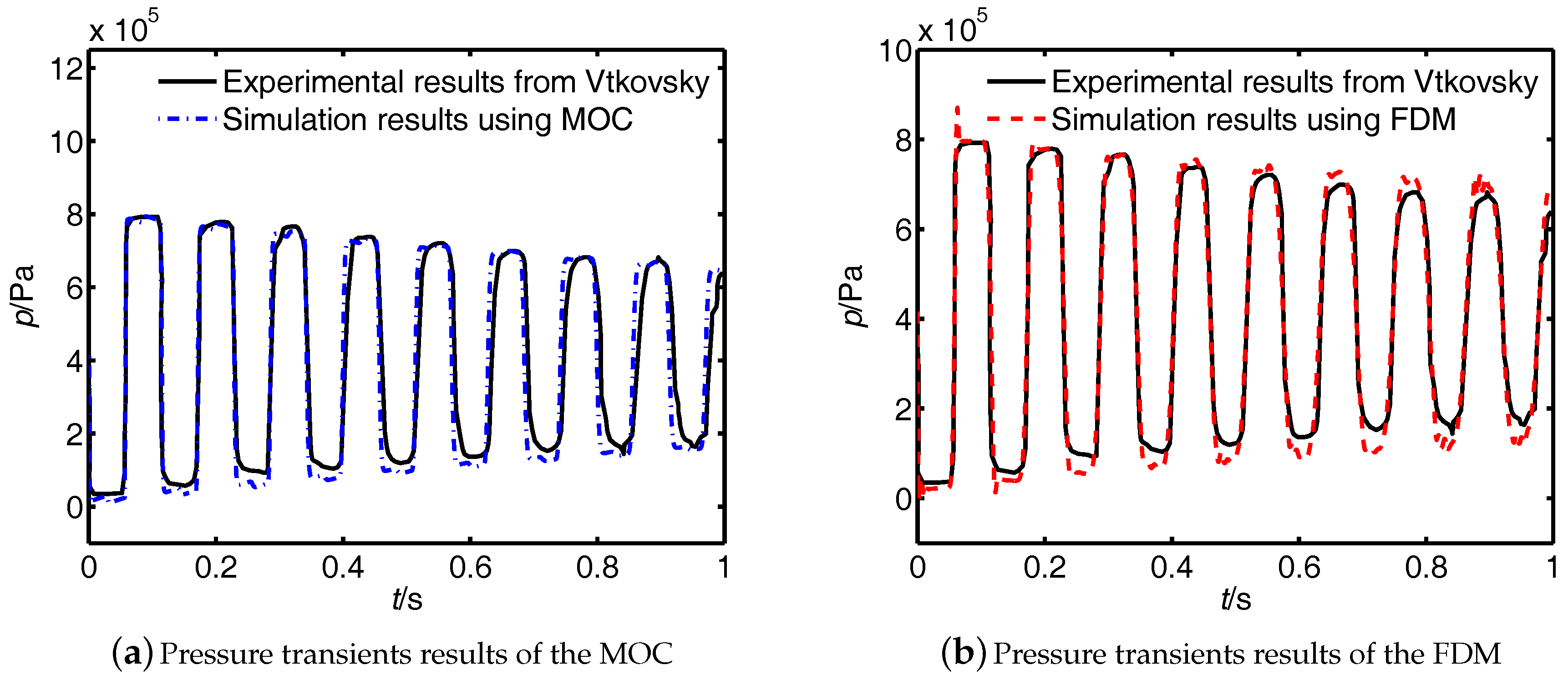
The experimental results of the transient pressure pulsations close to the valve in the horizontal downstream pipeline are given by Vitkovsky et al. [35] and the related parameters of the tested pipeline are listed in

Table 2. Parameters of pressure transients without cavitation on the downstream side of the valve.

Parameter	Value
Upstream tank pressure $p_{resu}$ (bar)	4.25
Downstream tank pressure $p_{resd}$ (bar)	4.22
Pipe radius $r_0$ (mm)	11.05
Pipe length L (m)	37.2
Water density $\rho$ ($\mathrm{kg}/{\mathrm{m}}^3$)	1000
Initial velocity $v_0$ (m/s)	0.3
Acoustic velocity in the fluid $c_0$ (m/s)	1319

. Here, the element number n is selected as 30 in the simulation. The sensitivity of this element number n has been discussed in [13]. The corresponding experimental results of transient pressure pulsations close to the valve are shown as the solid line in Figure 5.

Figure 5 denotes that, in the downstream pipeline, the pressure at the vicinity of the valve is reduced quickly when the valve is closed. At the same time, the negative pressure wave propagates to the downstream tank. Then, the positive pressure wave is reflected from the downstream tank and travels back to the valve, which leads to the first positive pressure peak. This process may be repeated several times before the fluid energy is dissipated due to the frictional force of the pipeline.

As shown in the experimental results, from 0 to 1 s, the attenuated peaks of the pressure pulsations are decreased very slowly. Because of the lower frictional force, the magnitudes of the pressure peaks decay slower in water, which is different from the corresponding pressure transient results with the working fluid as hydraulic oil (Jiang et al. [13]). Thus, if the pressure pulsations are always greater than the saturated vapor pressure, no cavitation forms.

For comparison, the simulation results of MOC are illustrated as the dash-dotted line in Figure 5a. The simulation results of the FDM platform are presented as the dashed line in Figure 5b. It can be seen that, from 0.4 to 1 s, the phase difference between the MOC simulation and the experimental results is more obvious. However, the simulation results of the FDM are still consistent with the experimental pressure results.

To further compare the two predictive methods, the error between the simulation and the experimental results was evaluated by the percentage of the integral of absolute difference (IAD) as follows (Rabie et al. [36]):

$$IAD=\frac{\underset{0}{\overset{T}{\int }}\left|p_{Lth}-p_{L\exp }\right|dt}{p_{Lss}T}\times 100\%.$$

(21)

The IAD results of the two predictive methods in the three cases are listed in

Table 3. The integral of absolute difference (IAD) of the method of characteristics (MOC) and the finite difference method (FDM).

Case	${\mathit{p}}_{\mathbf{Lss}}$ (bar)	IAD of MOC	IAD of FDM
1	$4.22$	0.91%	0.05%
2	$0.98065$	2.75%	2.47%
3	$4.90325$	12.39%	10.84%

. In Case 1, the final steady-state pressure at the valve is equal to the downstream tank pressure (4.22 bar), and the IAD of the FDM is about 0.05%. Thus, the simulation of the FDM is consistent with the experimental result, which is superior to the MOC (IAD = 0.91%).

4.2. Case 2: Pressure Transients with Cavitation on the Downstream Side of Valve

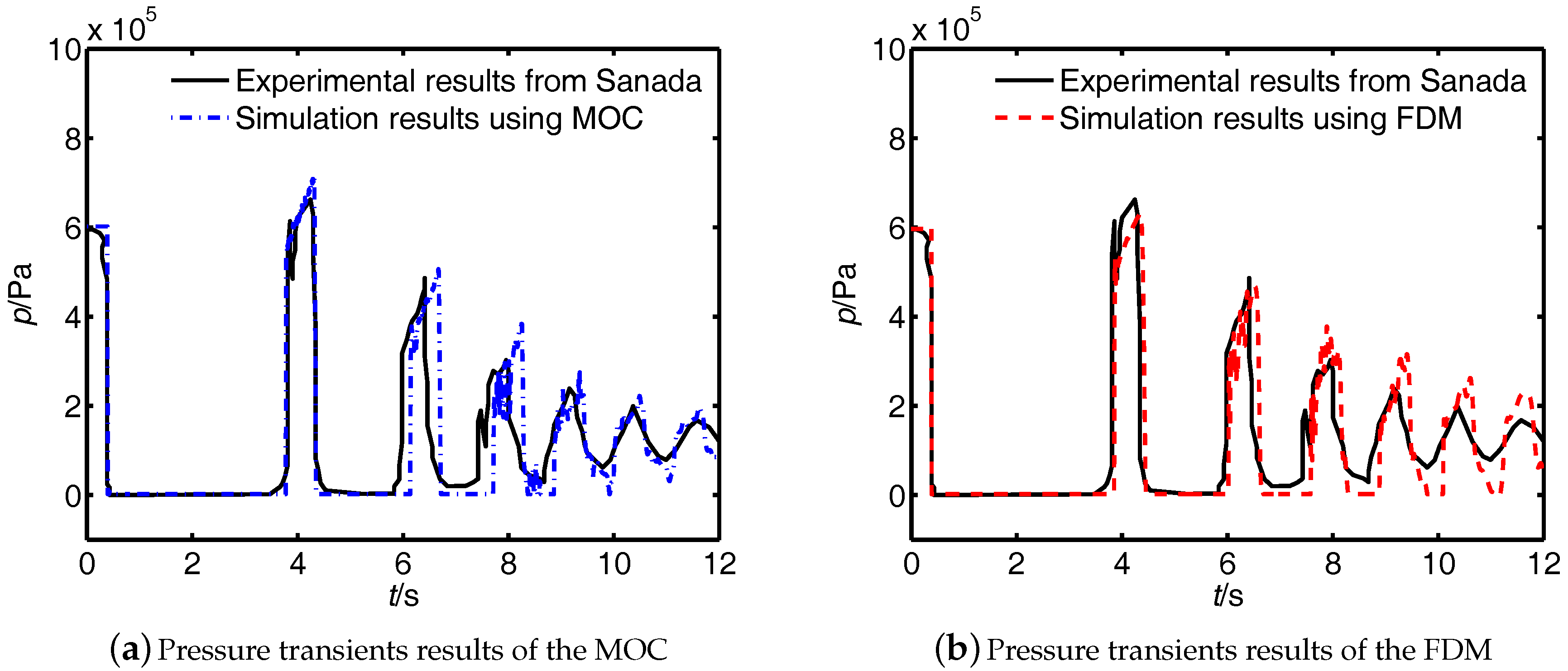
The case of transient pressure pulsations with cavitation in the horizontal downstream pipeline was also investigated. Some experimental parameters from Sanada et al. [37] are listed in

Table 4. Parameters of pressure transients with cavitation on the downstream side of the valve.

Parameter	Value
Upstream pressure $p_{resu}$ (bar)	6.55164
Downstream pressure $p_{resd}$ (bar)	0.98065
Pipe radius $r_0$ (mm)	7.6
Pipe length L (m)	200
Water density $\rho$ ($\mathrm{kg}/{\mathrm{m}}^3$)	1000
Initial velocity $v_0$ (m/s)	1.5
Viscosity of the fluid $c_0$ (cP)	1

. The corresponding experimental results are shown as the solid line in Figure 6. As the valve is quickly closed, the pressure reduces and stays at vapor pressure for about 3 s. The pressure then drops again and stays at vapor pressure for about 1.5 s. For the third time, the pressure falls and stays at vapor pressure for about 1 s.

The results obtained from the MOC and the FDM are also shown in Figure 6. It is clear that obvious differences exist between the MOC simulation and the experimental results, especially in terms of the phase differences of the subsequent peaks. However, the results of the FDM via Matlab/Simulink Platform are consistent with the experimental results.

As listed in Table 3, for Case 2, the final steady-state pressure at the valve is 0.98065 bar, which is equal to the downstream tank pressure. Different from Case 1, the two predictive methods have similar effects (the IADs of the two predictive methods are 2.75% and 2.47%).

The corresponding cavitation volumes in the element close to the valve predicted by the FDM and the MOC are shown in Figure 7. The trends of vaporous cavitation volume under three cases are listed in

Table 5. Trends of cavitation volume.

Times	Method	MOC (case 1)	FDM (case 1)	MOC (case 2)	FDM (case 2)	MOC (case 3)	FDM (case 3)
1st time	start time (s)	–	–	0.40	0.38	0.60	0.65
	end time (s)			3.77	3.87	1.21	1.24
	duration (s)			3.37	3.49	0.61	0.59
	maximum volume time (s)			2.32	2.11	1.08	1.21
	maximum volume (${\mathrm{m}}^3$)			$1.401\times {10}^{-4}$	$1.372\times {10}^{-4}$	$1.305\times {10}^{-5}$	$3.955\times {10}^{-6}$
2nd time	start time (s)	–	–	4.34	4.37	2.05	1.98
	end time (s)			6.14	6.03	2.17	2.23
	duration (s)			1.80	1.66	0.12	0.25
	maximum volume time (s)			5.12	5.73	2.15	2.21
	maximum volume (${\mathrm{m}}^3$)			$4.155\times {10}^{-5}$	$1.892\times {10}^{-5}$	$1.281\times {10}^{-6}$	$6.785\times {10}^{-7}$
3rd time	start time (s)	–	–	6.72	6.54	–	–
	end time (s)			7.71	7.62
	duration (s)			0.99	1.08
	maximum volume time (s)			7.46	6.76
	maximum volume (${\mathrm{m}}^3$)			$1.009\times {10}^{-5}$	$1.535\times {10}^{-6}$

, which includes the cavitation start time, the end time, the duration, the maximum volume, and the corresponding time points.

Similar to the MOC, the FDM is also able to track the trends of cavitation volume. The results indicate that the computed pressure peak declines to the saturated vapor pressure after the valve is rapidly closed and after cavitation forms. However, this new cavitation collapses at 3.87 s (FDM) and 3.77 s (MOC). The maximum volumes of cavitation first are $1.372\times {10}^{-4}$ ${\mathrm{m}}^3$ (FDM) and $1.401\times {10}^{-4}$ ${\mathrm{m}}^3$ (MOC). When the pressure declines again, cavitation is generated again, but it is much smaller ($1.892\times {10}^{-5}$ ${\mathrm{m}}^3$ from the FDM and $4.155\times {10}^{-5}$ ${\mathrm{m}}^3$ from the MOC) than the first instance. Once again, cavitation collapses at the arrival of the third pressure peak. The durations of the third cavitation is 1.08 s (FDM) and 0.99 s (MOC). Thus, over this short period (12 s), the cavitation demonstrates generation and collapse three times.

4.3. Case 3: Pressure Transients with Cavitation on the Upstream Side of the Valve

Sanada et al. [37] also provided parameters of tested pipelines in the case of transient pressure pulsations in a horizontal upstream pipeline, as listed in

Table 6. Parameters of pressure transients with cavitation on the upstream side of the valve.

Parameter	Value
Upstream pressure $p_{resu}$ (bar)	4.90325
Downstream pressure $p_{resd}$ (bar)	0.98065
Pipe radius $r_0$ (mm)	7.6
Pipe length L (m)	200
Water density $\rho$ ($\mathrm{kg}/{\mathrm{m}}^3$)	1000
Initial velocity $v_0$ (m/s)	1.45
Viscosity of fluid $c_0$ (cP)	1

. Compared with Case 2 listed in Table 4, the parameters of the test pipeline are the same, except for the values of the upstream pressure and the initial velocity.

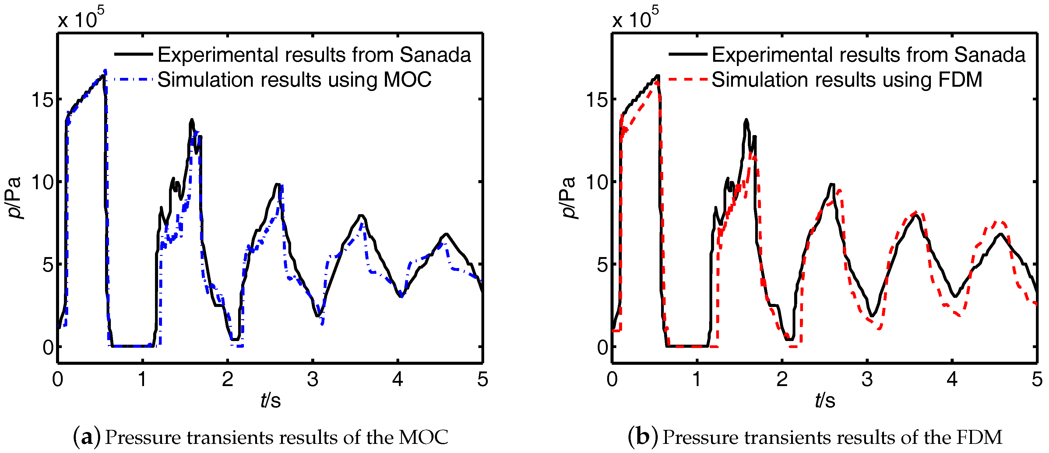
Figure 8 demonstrates the sequence of pressures with cavitation caused by instant valve closure. Compared with the pressure pulsations in the downstream pipeline, after a sudden valve closure, the fluid is brought to rest, firstly causing a high pressure peak at the upstream side of the valve.

Experimental results from Sanada (the solid line in Figure 8) show that the initial pressure at the valve is about $16\times {10}^5$ Pa when the valve is closed. It then reduces to the vapor pressure and keeps a steady state until about 0.5 s. Upon collapse of the cavitation, another pressure wave is generated at the valve. The subsequent pressure peak is reduced because of the friction force in the pipeline.

The figure also shows the simulation results from the MOC and the FDM. For the case of the upstream side of the valve, the final steady-state pressure at the valve is equal to the upstream tank pressure (4.90 bar). As listed in Table 3, the IADs of the MOC and the FDM are 12.39% and 10.84%. It is clear that the results of the FDM has much better consistency with the experimental results than those using the MOC.

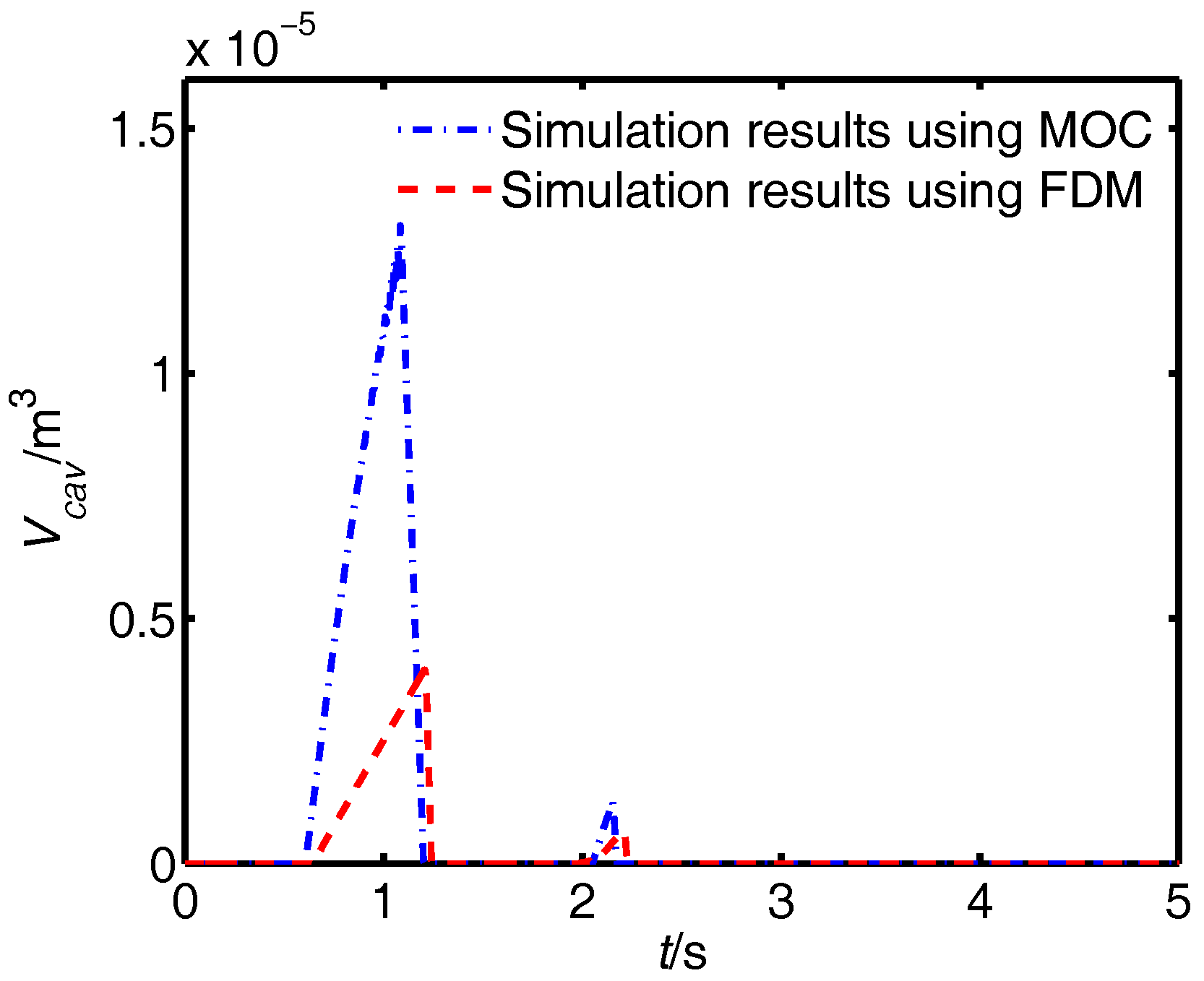
The corresponding cavitation volumes in the element close to the valve are shown in Figure 9. The maximum size of the vaporous cavity is $3.955\times {10}^{-6}$ ${\mathrm{m}}^3$ (the duration is about 0.59 s) using the FDM and $1.305\times {10}^{-5}$ ${\mathrm{m}}^3$ (the duration is about 0.61 s) using the MOC. When the pressure reduces to vapor pressure again, using the FDM, the second cavity has a volume of $6.785\times {10}^{-7}$ ${\mathrm{m}}^3$ and a duration of 0.25 s; however, using the MOC, the cavity has a volume of $1.281\times {10}^{-6}$ ${\mathrm{m}}^3$ and a duration of 0.12 s.

As listed in Table 5, based on a comparison between Case 2 and Case 3, the durations of cavitation are much longer and the maximum cavitation volumes are larger on the downstream side of the valve. It is clear that cavitation is more likely to occur on the downstream side of the valve.

5. Conclusions

To reveal the mechanism of cavitation growth and collapse both on upstream and downstream of the water-hydraulic pipeline, this paper proposes the finite difference method (FDM) for determining the transient pressure to estimate pipeline pressure transients caused by sudden changes in fluid velocity. Firstly, the dynamic model of cavitation volume was derived during pressure transients. Then, the cavitation appearance durations and volume changes were analyzed. Furthermore, the frictional force model with the steady and frequency-dependent unsteady items were constructed in the proposed dynamic model. By referring to experimental results in [35,37], the simulation results of two computation methods were verified to indicate that the proposed FDM for transient pressure estimation has the following two advantages:

(i) The FDM is consistent with experimental results, which is improvement over the MOC in terms of the phase differences and magnitudes of the pressure peaks.

(ii) The FDM estimates not only the magnitudes of the pressure peaks but also the changes in cavitation volume to adapt the transient pressure both with and without cavitation. By statistical results, the IAD values of the FDM are much more favorable than that of the MOC.

However, the aforementioned discussion assumes that no air is released during cavitation. In fact, water usually contains some dissolved air or gas. If the pressure declines under the saturation pressure, especially under vapor pressure with agitation, then a certain amount of air will be released as gas bubbles. Thus, these effects of gas bubbles on pressure transients with cavitation will be investigated in the near future.

References

- Kojima, E.; Shinada, M.; Shindo, K. Fluid transient phenomena accompanied with column separation in fluid power pipeline. Bull. JSME 1984, 27, 2421–2429. [Google Scholar] [CrossRef]
- Chaudhry, M.H.; Bhallamudi, S.M.; Martin, C.S.; Naghash, M. Analysis of transient pressures in bubbly, homogeneous, gas-liquid mixtures. J. Fluids Eng.-Trans. ASME 1990, 112, 225–231. [Google Scholar] [CrossRef]
- Chaudhry, M.H. Applied Hydraulic Transients, 3rd ed.; Springer: New York, NY, USA, 2014. [Google Scholar]
- Guo, Q.; Zhang, Y.; Celler, B.G.; Su, S.W. Backstepping control of electro-hydraulic system based on extended-state-observer with plant dynamics largely unknown. IEEE Trans. Ind. Electron. 2016, 63, 6909–6920. [Google Scholar] [CrossRef]
- Guo, Q.; Zhang, Y.; Celler, B.G.; Su, S.W. State-constrained control of single-rod electrohydraulic actuator with parametric uncertainty and load disturbance. IEEE Trans. Control Syst. Technol. 2017. [Google Scholar] [CrossRef]
- Guo, Q.; Wang, Q.; Liu, Y. Anti-windup control of electro-hydraulic system with load disturbance and modeling uncertainty. IEEE Trans. Ind. Inform. 2017. [Google Scholar] [CrossRef]
- Guo, Q.; Yu, T.; Jiang, D. Robust H∞ positional control of 2-DOF robotic arm driven by electro-hydraulic servo system. ISA Trans. 2015, 59, 55–64. [Google Scholar] [CrossRef] [PubMed]
- Shu, J.J.; Burrows, C.R.; Edge, K.A. Pressure pulsation in reciprocating pump piping systems Part 1: Modelling. Proc. Inst. Mech. Eng. Part I 1997, 211, 229–237. [Google Scholar] [CrossRef]
- Shu, J.J. A finite element model and electronic analogue of pipeline pressure transients with frequency-dependent friction. J. Fluids Eng. 2003, 125, 194–199. [Google Scholar] [CrossRef]
- Shu, J.J. Modeling vaporous cavitation on fluid transient. Int. J. Press. Vessels Pip. 2003, 80, 187–195. [Google Scholar] [CrossRef]
- Bergant, A.; Simpson, A.R. Pipeline column separation flow regimes. J. Hydraul. Eng. 1999, 125, 835–848. [Google Scholar] [CrossRef]
- Bergant, A.; Simpson, A.R.; Tijsseling, A.S. Waterhammer with column separation: A historical review. J. Fluids Struct. 2006, 22, 135–171. [Google Scholar] [CrossRef]
- Jiang, D.; Li, S.J. Simulation of hydraulic pipeline pressure transients accompanying cavitation and gas bubbles using Matlab/Simulink. In Proceedings of the 2006 ASME Joint U.S.-European Fluids Engineering Summer Meeting, Miami, FL, USA, 17–20 July 2006; pp. 657–665. [Google Scholar]
- Jiang, D.; Li, S.J.; Bao, G. Parameter identification of gas bubble model in pressure pulsations using genetic algorithms. Acta Phys. Sin. 2008, 57, 5072–5080. [Google Scholar]
- Jiang, D.; Li, S.J.; Edge, K.A.; Zeng, W. Modeling and simulation of low pressure oil-hydraulic pipeline transients. Comput. Fluids 2012, 67, 79–86. [Google Scholar] [CrossRef] [Green Version]
- Jiang, D.; Li, S.J.; Yang, P.; Zhao, T.Y. Frequency-dependent friction in pipelines. Chin. Phys. B 2015, 24, 034701. [Google Scholar]
- Shi, Y.; Wang, Y.; Cai, M.; Zhang, B.; Zhu, J. An aviation oxygen supply system based on a mechanical ventilation model. Chin. J. Aeronaut. 2018, 31, 197–204. [Google Scholar] [CrossRef]
- Shi, Y.; Zhang, B.; Cai, M.; Zhang, D. Numerical Simulation of volume-controlled mechanical ventilated respiratory system with two different lungs. Int. J. Numer. Methods Biomed. Eng. 2016, 33, 2852. [Google Scholar] [CrossRef] [PubMed]
- Shi, Y.; Zhang, B.; Cai, M.; Xu, W. Coupling Effect of Double Lungs on a VCV Ventilator with Automatic Secretion Clearance Function. IEEE/ACM Trans. Comput. Biol. Bioinform. 2017. [Google Scholar] [CrossRef]
- Shi, Y.; Wu, T.; Cai, M.; Wang, Y.; Xu, W. Energy conversion characteristics of a hydropneumatic transformer in a sustainable-energy vehicle. Appl. Energy 2016, 171, 77–85. [Google Scholar] [CrossRef]
- Sadafi, M.; Riasi, A.; Nourbakhsh, S.A. Cavitating flow during water hammer using a generalized interface vaporous cavitation model. J. Fluids Struct. 2012, 34, 190–201. [Google Scholar] [CrossRef]
- Karadžić, U.; Bulatović, V.; Bergant, A. Valve-Induced Water Hammer and Column Separation in a Pipeline Apparatus. J. Mech. Eng. 2014, 60, 742–754. [Google Scholar] [CrossRef]
- Iglesias-Rey, P.L.; Fuertes-Miquel, V.S.; Garcia-Mares, F.J.; Martínez-Solano, F.J. Characterization of Commercial Air Intake and Exhaust Valves. Tecnol. Cienc. Agua 2016, 7, 57–69. [Google Scholar]
- Fuertes-Miquel, V.S.; López-Jiménez, P.A.; Martínez-Solano, F.J.; López-Patiño, G. Numerical modelling of pipelines with air pockets and air valves. Can. J. Civ. Eng. 2016, 43, 1052–1061. [Google Scholar] [CrossRef]
- Majd, A.; Ahmadi, A.; Keramat, A. Investigation of Non-Newtonian Fluid Effects during Transient Flows in a Pipeline. J. Mech. Eng. 2016, 62, 105–115. [Google Scholar] [CrossRef]
- Zhou, L.; Wang, H.; Liu, D.Y.; Ma, J.J.; Wang, P.; Xia, L. A second-order Finite Volume Method for pipe flow with water column separation. J. Hydro-Environ. Res. 2017, 17, 47–55. [Google Scholar] [CrossRef]
- Wang, H.; Zhou, L.; Liu, D.Y.; Karney, B.; Wang, P.; Xia, L.; Ma, J.J.; Xu, C. CFD Approach for column separation in water pipelines. J. Hydraul. Eng. 2016, 142, 04016036. [Google Scholar] [CrossRef]
- Himr, D. Investigation and numerical simulation of a water hammer with column separation. J. Hydraul. Eng. 2016, 141, 04014080. [Google Scholar] [CrossRef]
- Wylie, E.B.; Streeter, V.L.; Suo, L.S. Fluid Transients in Systems; Prentice-Hall: Englewood Cliffs, NJ, USA, 1993. [Google Scholar]
- Pettersson, M.; Weddfelt, K.; Palmberg, J.O. Modelling and measurement of cavitation and air release in a fluid power piston pump. In Proceedings of the Third Scandinavian International Conference on Fluid Power, Linköping, Sweden, 25–26 May 1993; p. 113. [Google Scholar]
- Harris, R.M.; Edge, K.A.; Tillley, D.G. The suction dynamics of positive displacement axial piston pumps. J. Dyn. Syst. Meas. Control 1994, 116, 281–287. [Google Scholar] [CrossRef]
- Zielke, W. Frequency-dependent Friction in Transient Liquid Flow. J. Basic Eng. 1968, 90, 109–115. [Google Scholar] [CrossRef]
- Trikha, A.K. Efficient Method for Simulation Frequency-dependent Friction in Transient Liquid Flow. J. Fluids Eng. 1975, 97, 97–105. [Google Scholar] [CrossRef]
- Taylor, S.E.M.; Johnston, D.N.; Longmore, D.K. Modeling of transient flow in hydraulic pipelines. Proc. Inst. Mech. Eng. Part I 1997, 211, 447–456. [Google Scholar]
- Vitkovsky, J.P.; Bergant, A.; Simpson, A.R.; Martin, M.A.; Lambert, F. Systematic evaluation of one-dimensional unsteady friction models in simple pipelines. J. Hydraul. Eng. 2006, 132, 696–708. [Google Scholar] [CrossRef]
- Rabie, M.G.; Rabie, M. Fluid Power Engineering; McGraw-Hill Education: New York, NY, USA, 2009. [Google Scholar]
- Sanada, K.; Kitagawa, A.; Takenaka, T. A study on analytical methods by classification of column separations in a water pipeline. Bull. JSME 1990, 56, 585–593. [Google Scholar] [CrossRef]
Figure 1.
Tank-pipeline-valve system.