Induction Thermography for Surface Crack Detection and Depth Determination


Institute for Automation, University of Leoben, Leoben A-8700, Austria
Appl. Sci. 2018, 8(2), 257; https://doi.org/10.3390/app8020257
Submission received: 15 December 2017
/
Revised: 2 February 2018
/
Accepted: 6 February 2018
/
Published: 9 February 2018
(This article belongs to the Special Issue Novel Ideas for Infrared Thermography also Applied in Integrated Approaches)
Abstract
:In the last few years, induction thermography has been established as a non-destructive testing method for localizing surface cracks in metals. The sample to be inspected is heated with a short induced electrical current pulse, and the infrared camera records—during and after the heating pulse—the temperature distribution at the surface. Transforming the temporal temperature development for each pixel to phase information makes not only highly reliable detection of the cracks possible but also allows an estimation of its depth. Finite element simulations were carried out to investigate how the phase contrast depends on parameters such as excitation frequency, pulse duration, material parameters, crack depth, and inclination angle of the crack. From these results, generalized functions for the dependency of the phase difference on all these parameters were derived. These functions can be used as an excellent guideline as to how measurement parameters should be optimized for a given material to be able to detect cracks and estimate their depth. Several experiments on different samples were also carried out, and the results compared with the simulations showed very good agreement.
1. Introduction
Induction heating is a well-known technique, as it is very efficient, fast, clean and accurately controlled [1]. Nowadays, it is not only used in the industry, but also for domestic applications, as induction cookers, and for medical purposes, as hyperthermia therapy [1].
In the case of induction thermography, the sample to be inspected is placed inside or close to an induction coil. During and after applying a short heating pulse, which is usually between 50 ms and 1 s, heat will be induced inside the material and an infrared camera records the temperature distribution. Evaluation of the temperature images and their temporal changes represents an excellent technique for crack detection, as it is a non-destructive, contact-free technique and can be very well fully automated using image processing methods.
In the last few years, several investigations have been published by different groups proving the applicability of this method. The first industrial application was reported around 30 years ago [2]. Steel bars and billets have been tested for surface cracks during motion through an induction coil and by evaluating the signal of four infrared line scanners placed around the steel bar. In the last 20 years, FPA (focal-plane-array) cameras became more powerful and dropped in price, maintaining more scientific research in the area of thermographic inspection [3]. Inductive thermography is one of the active thermography methods, which have been studied and developed by several groups in the few last years. The working group around Busse investigated induction thermography to detect subsurface defects in steel and in CFRP (carbon fiber reinforced polymer) samples in a modulated way (lock-in technique) and with pulse heating (burst thermography) [4]. Aluminum fatigue surface cracks have been also detected using the lock-in technique [5]. Analytical and numerical models [6,7,8] have been set up for modeling cracks perpendicular to the surface in steel materials. In these simplified models, the cracks were modeled either as a long notch or as a short slot going through the whole sample thickness [7,8]. Experimental results for surface crack detection with induction thermography have been reported by several groups in different ferro-magnetic samples, for example, in forged parts [9,10] and in rail surfaces [11,12]. As these head checks lay typically inclined to the surface, further numerical models have been set up for angular defects [12,13,14]. As induction thermography became an important NDT (non-destructive testing) method for detecting surface cracks in industrial applications [15], many efforts have been undertaken [16] to set up a standard [17].
This paper presents several investigations on the influence of different experimental and material parameters on surface crack detection. However, important emphasis was placed on how the position is obtained and on how the depth of a crack can be estimated from the detected signal. In the first part of the paper, finite element simulations are carried out to show how experimental parameters, such as excitation frequency and pulse duration, as well as material parameters and the properties of the crack, such as depth and inclination angle, affect the results. Four different cases were investigated: cases where the penetration depth was small, cases where the penetration depth was similar large as the crack depth, and these in combination with cases where the crack was perpendicular to the surface, and cases where the crack lay under a given inclination angle. For each of these combinations, experimental results are presented. Several samples with artificial and “natural” cracks were measured, and the results are compared with the simulated ones.
The main goal of this study was to derive general, normalized functions for vertical cracks, which are independent of the material parameters and depend only on two ratios: the ratio of the crack depth to the penetration depth, and the ratio of the crack depth to the thermal diffusion length. In the case of inclined cracks, the angle affects the results. These generalized functions have the goal to provide a guideline as to how the experimental parameters can be optimized for a given material to reliably detect surface cracks and estimate their depth.
2. The Models
In induction heating, eddy currents are induced in an electrically conductive sample. This current flows directly below the surface of the material in a shallow depth. Due to the ohmic resistance of the sample heat, the so-called Joule heat is generated below the surface inside the material. The penetration depth of the induced eddy current can be determined by
where µ0 denotes the permeability of vacuum with the value of 4π10−7 Vs/Am; µr is the relative magnetic permeability of the material; σ is its electrical conductivity; f is the excitation frequency. This penetration depth is strongly influenced, on one hand, by the material properties, and on the other hand, by the excitation frequency. Table 1 summarizes these values for two materials.
This formula is only valid for the ideal case of a semi-infinite plane surface; otherwise, the eddy current distribution and its penetration depth is affected by the sample geometry.
A non-uniform heat distribution initiates a diffusion process to equalize the temperature differences. Generally, a diffusion process, i.e., heat diffusion, can be characterized by the diffusion length, describing approximately how far the heat flows in a given time t.
where κ denotes the thermal diffusivity of the material.
In the case of ferro-magnetic material at a typical excitation frequency of 200 kHz, the penetration depth is negligibly small and can be well estimated as a surface heat flux. In a simplified model, assuming that the eddy current cannot flow through the crack and flows around it, the heating is applied not only to the surface of the sample but also to the sides of the crack. An analytical model was developed [6,18,19] for cases where a vertical crack is heated with a surface heat flux. This model describes very well the temperature distribution around a crack due to this additional heating. The sound surface can usually be modeled as a semi-infinite body, thereby the temperature increases as
where Q denotes the applied surface heat flux. At the position of the crack with depth d, the temperature is calculated according to [18].
where Ei( ) is the so-called exponential integral function. The relative temperature contrast can be calculated for this case as
where α denotes the ratio
As can be seen, the contrast depends only on the ratio of the crack depth d to the thermal diffusion length dth, whereby this second one contains the dependency on the heating duration time t, and the material dependent thermal diffusivity κ. If the ratio α = d/dth is large, then Tcrack(t) ~2 Tsound(t) and CR(t) becomes close to 1.
To model more complex problems, such as inclined cracks or when the penetration depth is not negligibly small, two types of finite element simulation models were set up using the multiphysics simulator ANSYS [20]:
- In the first model (simu.1), surface heat flux is directly applied to the crack sides and to the surface of the sample. The simulation calculates the temperature distribution during the heating pulse and in the cool-down phase after switching off the induction heating.
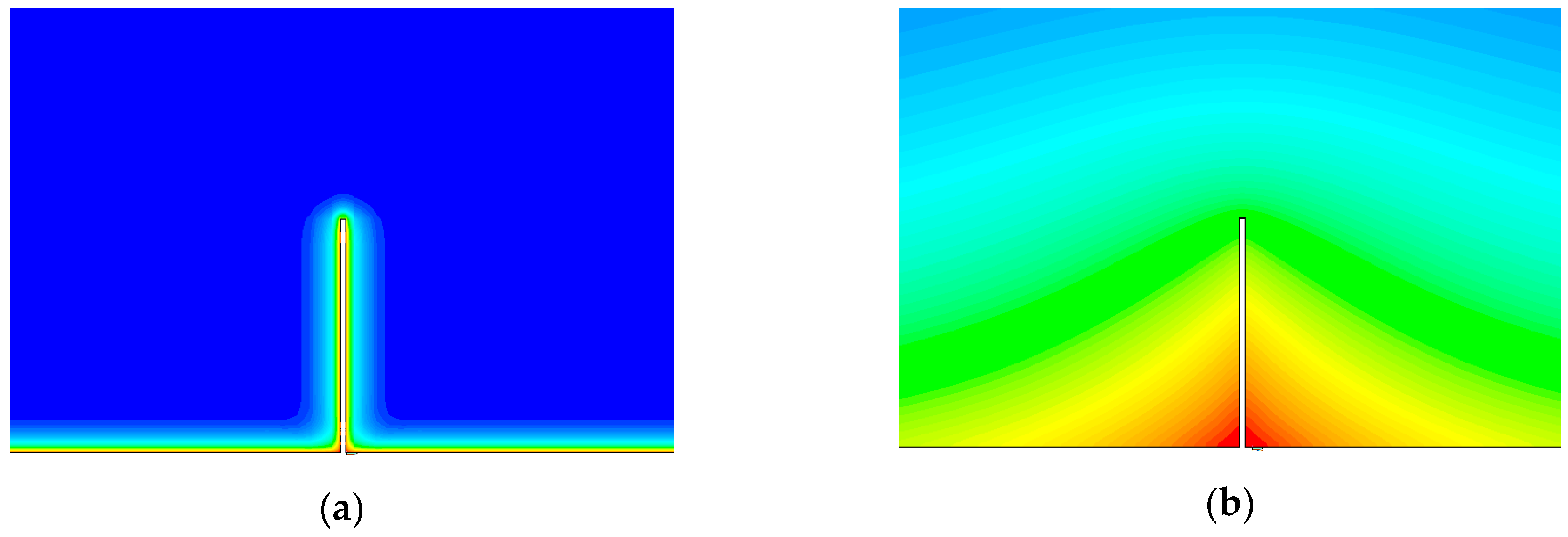
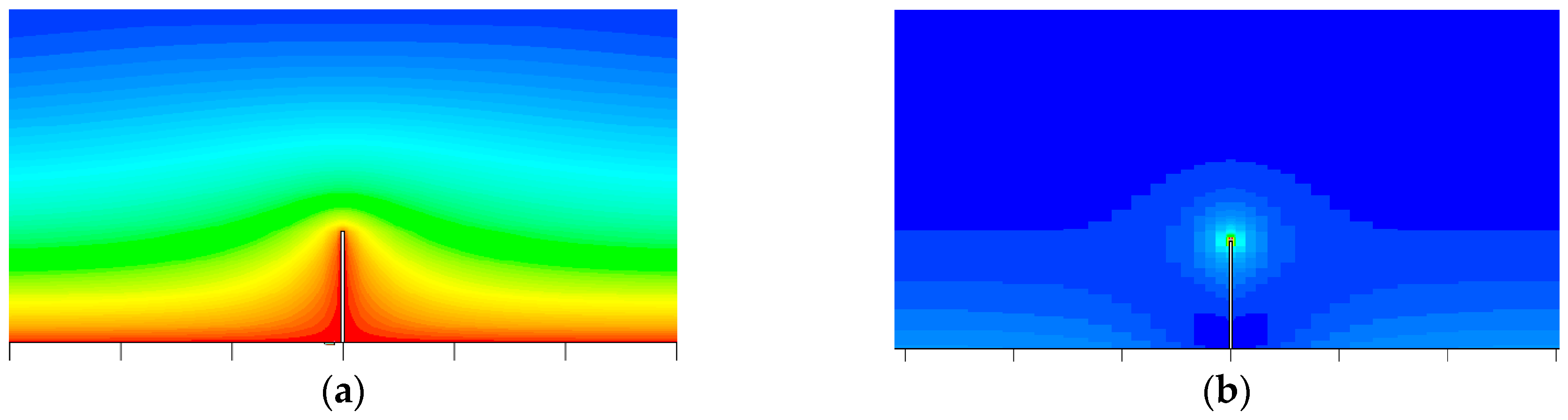
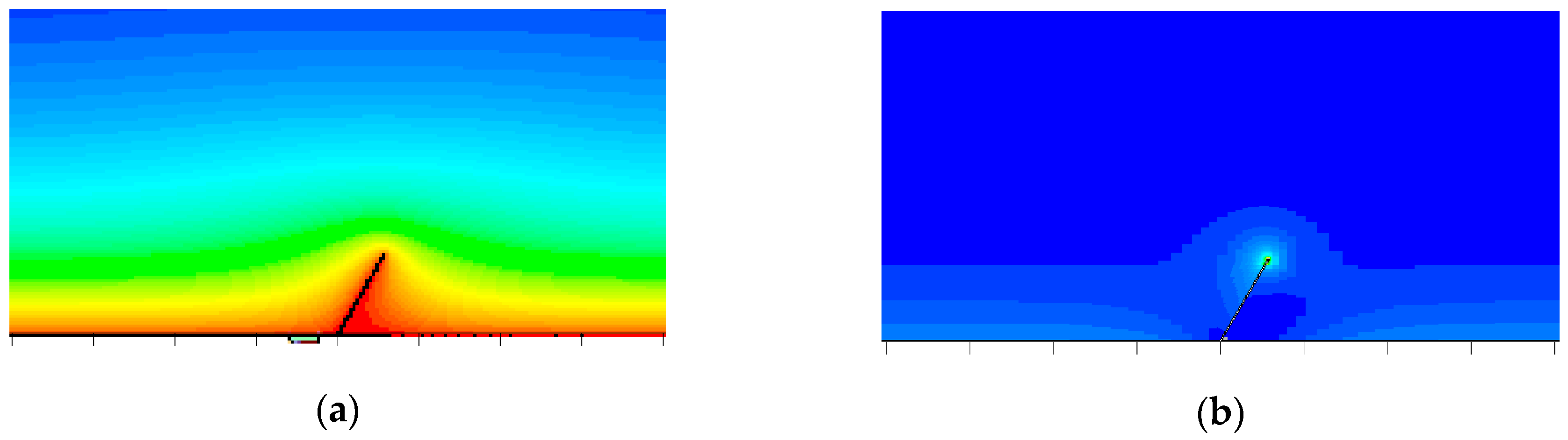
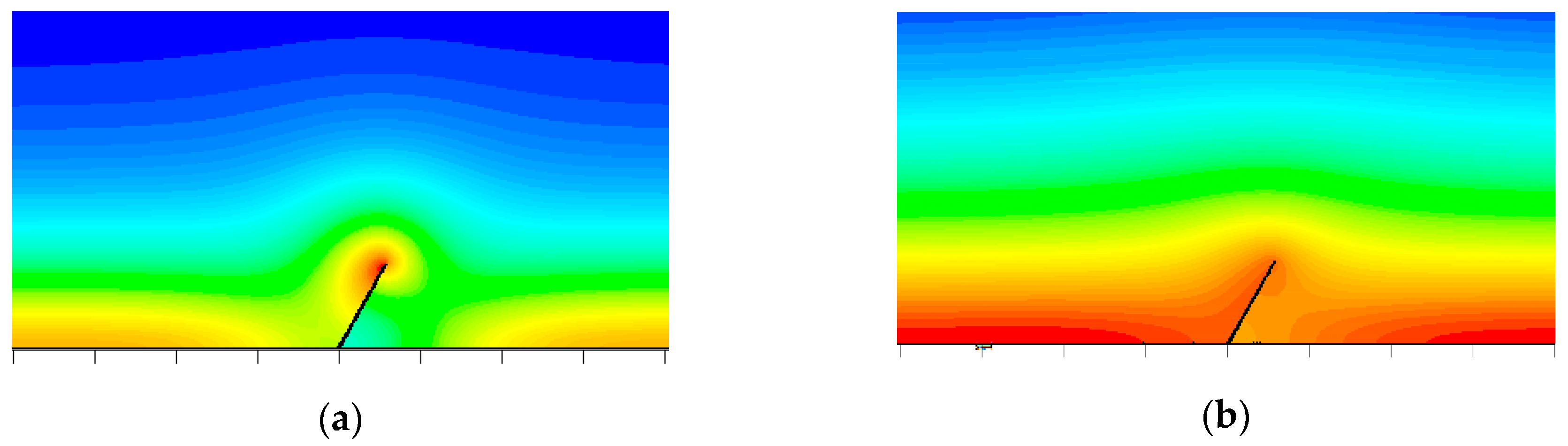
- In the second model (simu.2), the inductive heating itself is also simulated, and the eddy current distribution is determined by the model. Due to the generated heat and taking into account the heat diffusion, the temperature distribution is calculated. Figure 1 shows the Joule heating and the temperature distribution calculated by this simulation model. It can be well observed that the Joule heating follows the line of the crack, and due to the heat accumulation in the crack corners, the temperature becomes higher in this region.
In simu.1 and simu.2, the crack is assumed to be a long crack, thereby the models have been set up in 2D in a cross-section to the defect. The size of the models was 12 × 40 mm². In both model types, several parameters such as crack depth, heating pulse duration, and the inclination angle of the crack to the surface are varied. Table 2 summarizes the results of the models and for the cases to which they can be applied. In this study, the results for these four listed cases are presented and compared. Additionally, for these cases, measurement results are also shown and compared with the simulation models.
To prove the validity of the simu.2 models, the results were compared for small penetration depths with the results of simu.1. Furthermore, these were compared with the analytical model for the situation where the crack is perpendicular to the surface. On one hand, the simu.2 models can be used to calculate general cases, but on the other hand, these models are complex and require very fine gridding, so high computer resources and long calculation times are needed. Therefore, in praxis, the simplest model should always be used, which is still appropriate to handle a specific case.
It is worth noting that, in these models, only the heating due to the ohmic loss was considered. In ferro-magnetic materials, a loss due to hysteresis occurs. We also set up numerical models including this phenomenon, but our experience was that its effect on crack detection is negligibly small, so this was not included in the currently presented results. In the presented simulations, one constant value of magnetic permeability is considered. This is a simplified model, as the relative permeability value is a complex number and depends on the excitation frequency [21,22]. Since only whether a penetration depth smaller than the crack depth or a penetration depth comparable to crack depth is decisive, the exact value of the penetration depth has no direct impact on the obtained results of our evaluations. Therefore, higher order effects such as additional polarization/de-polarization losses due to hysteresis are not taken into account.
3. Vertical Cracks with Small Eddy Current Penetration Depth
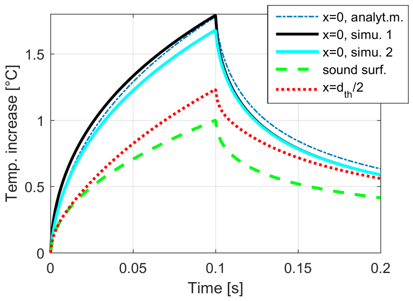
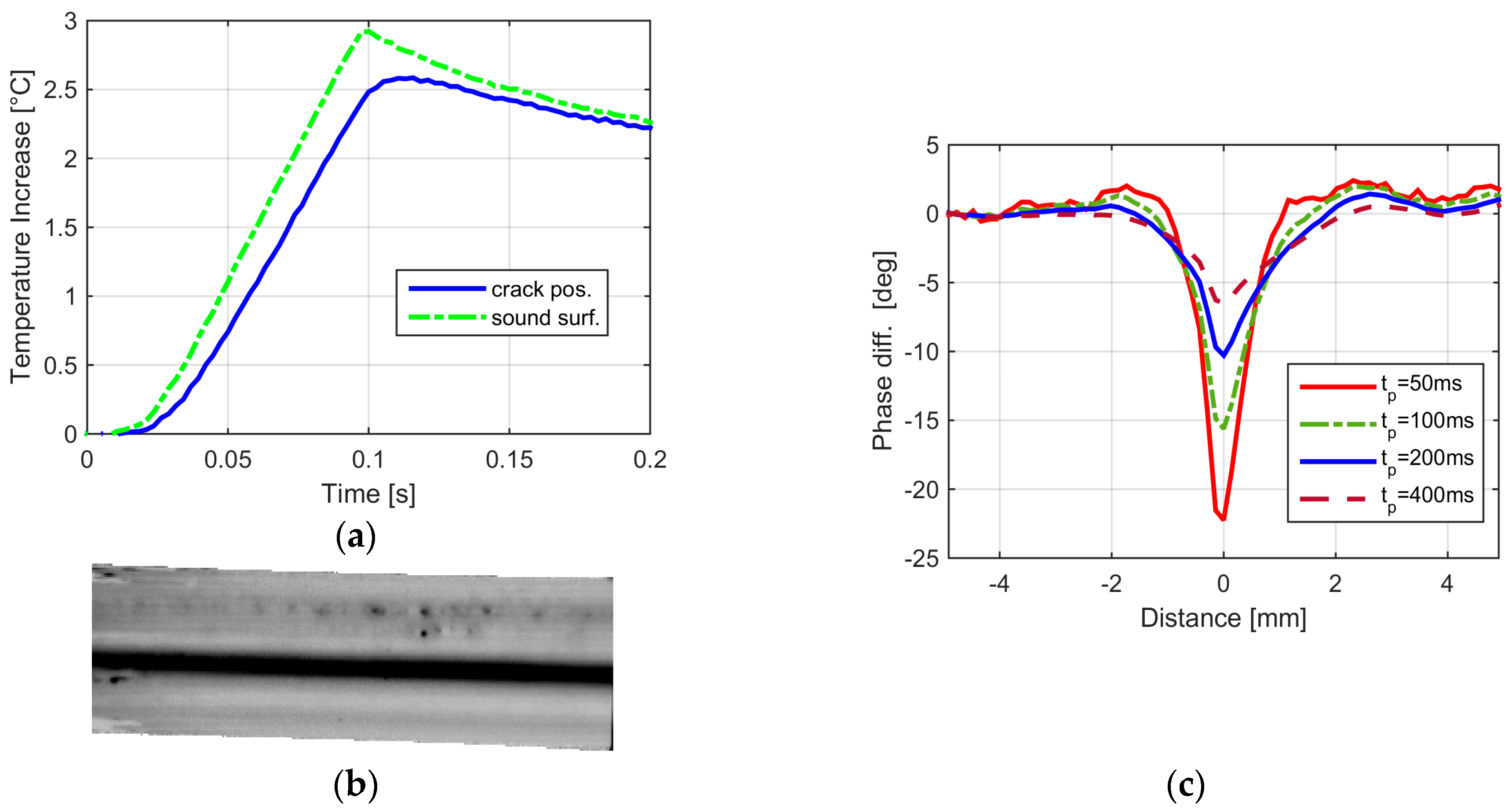
A vertical crack lies perpendicular to the surface. It is assumed to be a barrier to the electrical current, which flows along the crack sides, generating additional heating in this region (see also Figure 1a). The crack also hampers heat diffusion, accumulating heat in the corners (see Figure 1b). For ferro-magnetic materials, the eddy current penetration depth is negligibly small for high-frequency excitation and the results of all three models can be well compared. This comparison was done for several different crack depths and heating pulse durations, where a very good agreement was found. Figure 2 demonstrates the results for the same case already shown in Figure 1. The temperature at the sound surface increases like a square root function, which is similar to a semi-infinite large body (see Equation (3)). The temperature at the crack position increases to a higher value. The analytical model and simu.1 provide almost the same results, and simu.2 yields a slightly lower temperature. This difference becomes stronger if the penetration depth of the eddy current is larger, which will be explained in later sections.
Additionally, the temperature increase at the position x = dth/2, i.e., in the distance of half the thermal diffusion length, is also plotted in Figure 2. For a short time, after switching on the heating (t < 0.025 s = tpulse/4), the temperature increases in the same manner to that at the sound surface. As the additional heat flow from the crack reaches this position, the temperature here increases more than that at the sound surface.
The temperature distribution at the surface around the crack is shown in Figure 3a. The axis of abscissa shows a normalized distance, allowing for a time- and material-independent comparison. The temperature at the surface is perturbed around the crack up to a distance of 2dth, but this distance increases with time. A very reliable detection result can be achieved if not only one single temperature image at the end of the heating pulse is considered, but if the whole time-dependent sequence during heating and cool-down is evaluated to one phase image using Fourier transformation [18]:
where τ = tpulse + tcooldown and tcooldown is usually taken in the range of tpulse/2 and tpulse. In this study, tcooldown = tpulse was chosen, but also a selection of tcooldown = tpulse/2 leads to very similar results to the presented ones. The phase image provides an excellent measure for the rate of the heat flow, where it increases more quickly and more slowly. It is much less sensitive to disturbing factors, such as inhomogeneous heating or inhomogeneous emissivity values, and has a much higher signal-to-noise ratio [18]. In Figure 3b, the phase difference at the crack compared to the sound surface is depicted. At the crack position, the phase is higher than that at the sound surface, as the temperature here increases more quickly and decreases more quickly after the heating is switched off. The phase has a minimum around x = dth/2, as at this position, the temperature increases at the beginning with the same rate as at the sound surface, but due to additional heat flowing from the crack to this position, the temperature later increases at a higher rate. After switching off the heating, the temperature at this point remains higher due to the heat flow from the crack position.
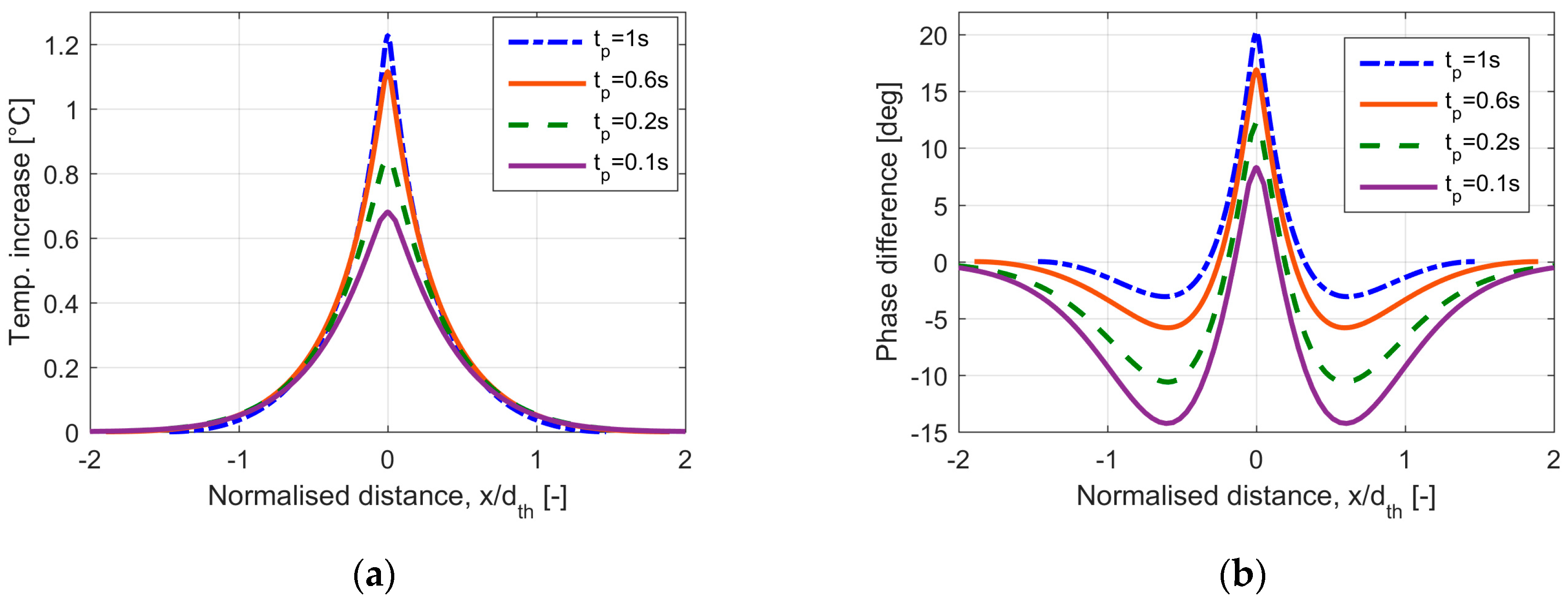
With increasing time, the additional heat around the crack spreads through the whole sample and becomes evenly distributed. The longer the heating pulse, the broader the heated region is around the crack. Figure 4a shows the temperature after different pulse lengths. As the diffusion length dth increases with time, the heated region around the crack also becomes broader and has an extension of 2dth on both sides of the crack. At the crack position, the phase is higher (see Figure 4b) than that at the sound surface and the minimum occurs around dth/2, which means that, with increasing pulse length, the width of the detectable phase signal of the crack increases.
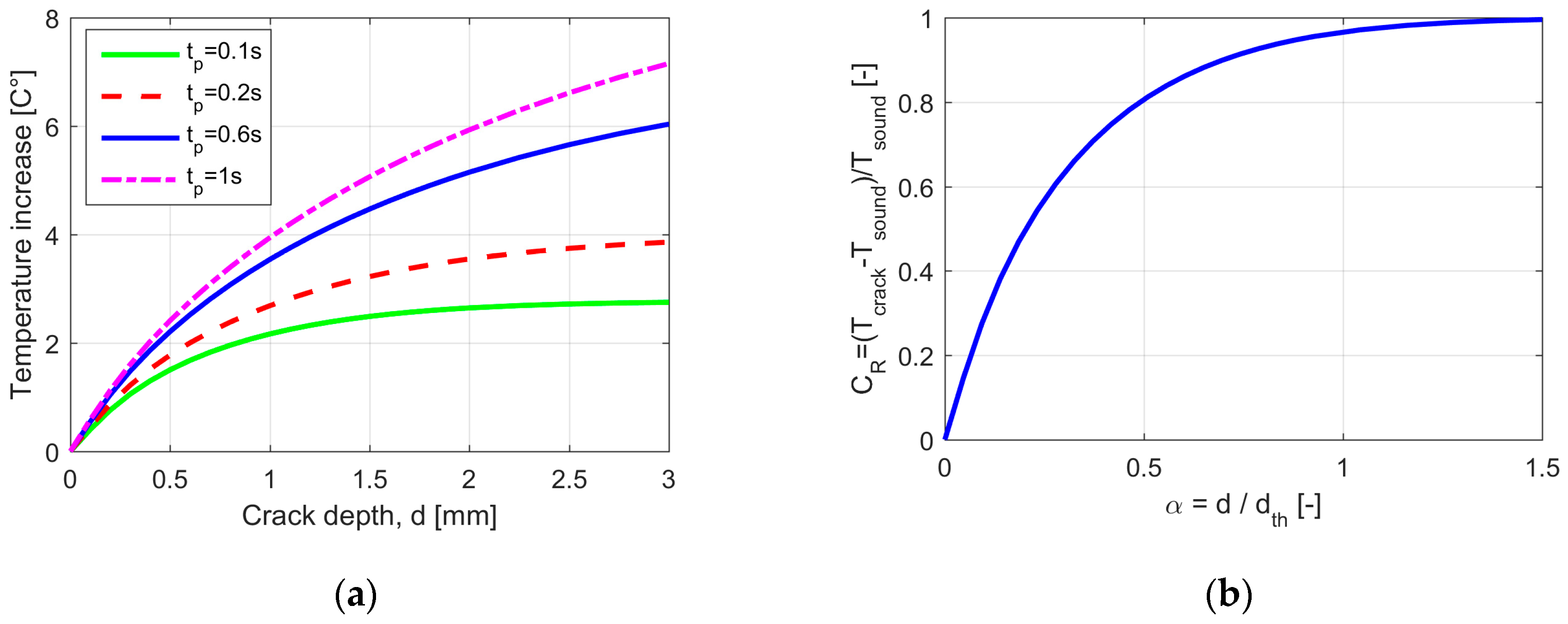
The deeper the crack, the more it represents a barrier for the eddy current and for heat diffusion. It can be seen from Equation (4) that the temperature at the crack position increases with depth d. Figure 5 compares the temperature and phase distribution around cracks with different depths. These simulations were carried out with all three models, and results of simu.2 are shown in the figure (f = 200 kHz, δ = 0.034 mm). Comparing the results of the three model types shows a very good agreement. How the temperature and the phase at the crack position depend on the crack depth is depicted in Figure 6a,b. In Figure 6c,d, the abscissa is α, which is the ratio of the crack depth to the thermal diffusion length. This means, e.g., that d = 1 mm and tpulse = 0.1 s results in dth = 2.16 mm and α = d/dth = 0.46; if tpulse = 1 s, then dth = 6.8 mm, and we have α = d/dth = 0.147. As the temperature increases monotonously with the crack depth, it would theoretically be suitable for determining the crack depth from measurements. On the other hand, inhomogeneous heating or variations in the emissivity, e.g., small scratches or ground surfaces, have a strong influence on the measured temperature, and the defect depth determination from the temperature increase is not reliable. In contrast, in the phase image, most of these factors become negligible, and the crack depth can be much more reliably determined.
According to Figure 6d, the phase contrast increases approximately up to a crack depth of dth/3 with a phase contrast of 27° at this depth. For deeper cracks, the phase contrast is saturated. This means that the optimal pulse duration is dependent on the crack depth, which should be resolved in the experiment. For example, for steel with tpulse = 0.1 s, one has a very good resolution of up to dth/3 = 2.16/3 mm = 0.72 mm and with tpulse =1 s up to dth/3 = 6.8/3 mm = 2.27 mm. If the pulse length is short, then shallow cracks are well resolved, but the same signal occurs for deeper cracks. If the pulse length is long, then deeper cracks can be resolved, but on the other hand, the signal and the resolution become low for shallow cracks.
4. Experimental Results for Vertical Cracks in Ferro-Magnetic Steel
For the experiments, a 10 kW induction generator with an excitation frequency of 200 kHz was used. The induction coil is a so-called Helmholtz coil consisting of two circular windings placed from each other at a distance (see Figure 7). This coil geometry has the advantage that the magnetic field in the region between the windings is approximately homogenous [10], and the induced eddy current flows roughly parallel to the coil circles. The workpiece to be inspected is placed in this middle part. We have manufactured several coils with different sizes and an appropriately sized coil is selected for each sample. An additional advantage of this coil geometry is that the infrared camera has an undisturbed view of the sample without occlusion by the coil. The generator works as a resonance circuit; the external capacitance and the inductivity of the coil determines the resonance frequency, which is then the working frequency of the generator.
It is important to note that the simulations and the measurements were set up in a way such that the induced eddy current flows perpendicular to the crack direction. Additional investigations were carried out on how the signal is influenced if this angle is less than 90° [10,23]. A possible setup was also presented using two Helmholtz coils with different excitation frequencies, whereby the detection becomes independent of the crack orientation.
The infrared camera has a cooled InSb detector, which is sensitive in the wavelength range 1.5–5 µm and whose frame rate is 383 images/s with a frame resolution of 320 × 256 pixels. The generator and the camera are controlled by PLC (programmable logic controller) to guarantee a reproducible and synchronized procedure.
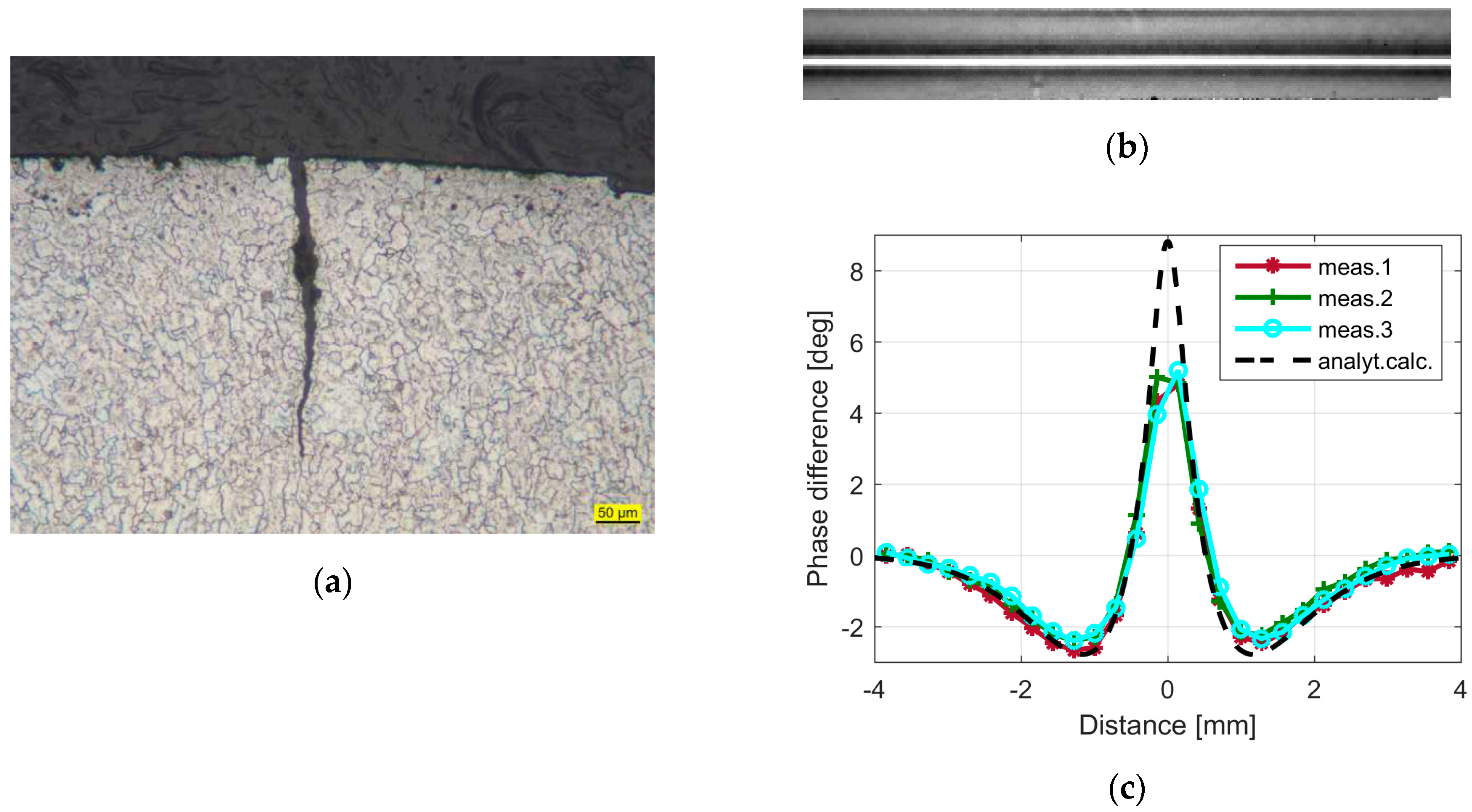
Figure 8 shows the results for a steel wire with a diameter of 10.8 mm. The crack is a very long defect, mainly along the whole wire with a constant depth. The wire was cut at one position and a microscopic cross section was made (see Figure 8a), showing a vertical crack with a depth of 0.35 mm. For the measurement, tpulse = 0.1 s was selected. The phase image is depicted in Figure 8b. The crack has a constant depth along the wire, as the phase contrast is very homogeneous. Figure 8c shows three profiles through this phase image, the distance between the positions of the profiles is about 23 mm, proving the homogeneity of the crack. In this diagram, the calculated phase profile for a depth of 0.35 mm is also plotted, showing very good agreement with the measured ones. In the experiment, the IR camera image has a resolution of 0.22 mm/pixel, so the phase peak at the crack position is not a perfect fit.
It is important to note that the induction generator cannot immediately switch the heating pulse on, but measurements show that, during the first approximately 40 ms, the induction current increases linearly. This behavior was also taken into consideration in the simulation model. Additionally, the wire with a diameter of 10.8 mm is not a “semi-infinite body” as considered in the models. Investigations of inductive heating for wires regarding the pulse length and the diameter have been published previously [24]. These results showed that for 0.1 s, the wire with a diameter of 10.8 mm behaves as a semi-infinite body.
In the simulation models, the crack is assumed to be a long crack, which can be modeled in 2D cross sections. The question arises how long a crack has to be so that the models remain valid. If a crack is short, then hot spots occur at its ends as the eddy current at the surface flows around the crack ends. Nevertheless, the 2D models are still valid in the middle part of the crack. Figure 9 shows a crack that is 12 mm long. The surface is ground in the region around the crack, therefore appearing shiny with a very low emissivity value. It was not necessary to blacken the surface; however, when the phase image is inspected, the crack becomes well visible. In Figure 9b, the measured phase profile is compared with the simulated one for a 1 mm crack depth. With the exception of the peak at the crack position, the agreement is good, and the crack depth is assumed to be approximately 1 mm.
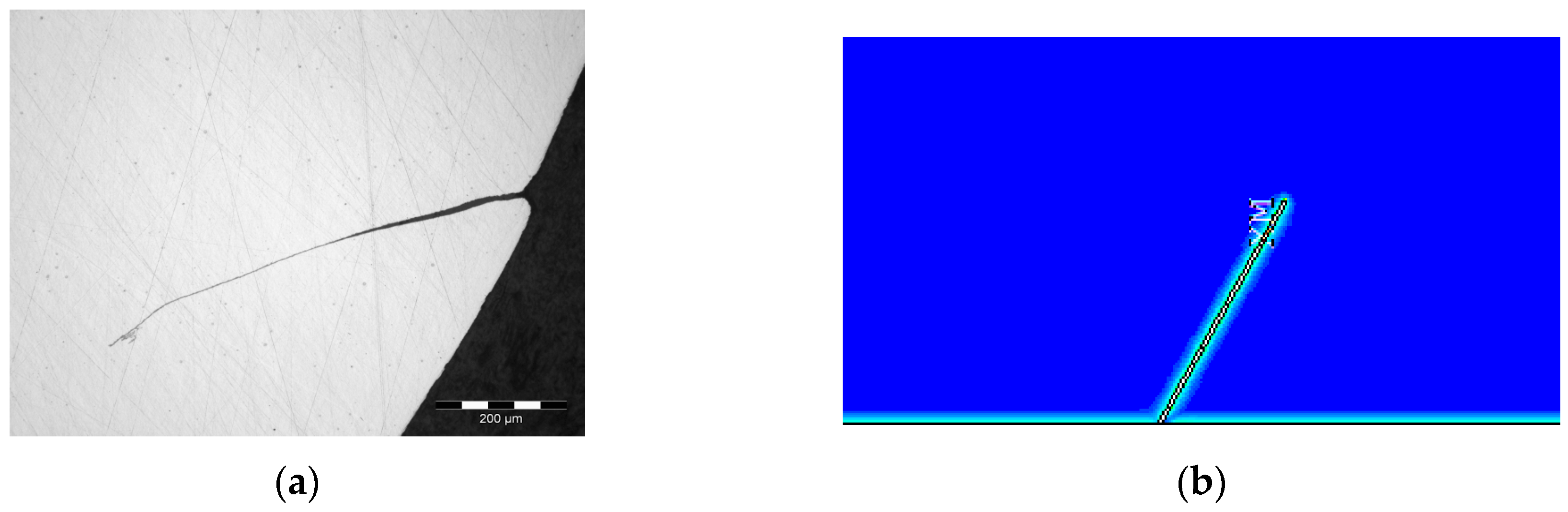
If the crack is significantly shorter with a length of about 1–3 mm, then only the hot spots at the crack ends are visible, and the 2D model is no longer applicable. The crack itself can be well localized from the hot spots at the ends, but crack depth estimation is very difficult, especially given that the depth along such a short crack length is most likely not homogeneous.
Another problem that may occur by fatigue cracks is that the two sides of the crack may slightly touch each other, creating a kind of electrical bridge for the eddy currents through the crack. Figure 10a shows the phase images of two samples with cracks having an approximate depth of 0.3 and 0.5 mm and a surface length of 10 mm. The defects were created artificially by bending [25] and have a width of a couple of µm. The phase contrast along the crack is not homogeneous and some brighter spots are visible, signaling small contact points between both faces of the crack. Nevertheless, a significant difference can be observed between the 0.3 and 0.5 mm crack depths. In Figure 10b, the phase profiles through the marked positions are plotted, which can be compared with the simulated signals shown in Figure 10c.
5. Inclined Cracks with Small Eddy Current Penetration Depth
In many cases, the crack does not lie perpendicular to the surface, but inclined with an angle. Typical defects are rolling or forging laps, as shown in Figure 11a. Such cracks can be simulated with the simu.1 and simu.2 models [14], as listed in Table 2 as “Case 3.” The results of both models were compared for several cases and showed good agreement. Figure 11b shows the simu.2 calculated Joule heating for ferro-magnetic steel around a crack depth of d = 1 mm and a θ = 30° inclination angle. As the eddy current penetration depth is very small (δ = 0.034 mm), the current and the Joule heating follow the line of the crack.
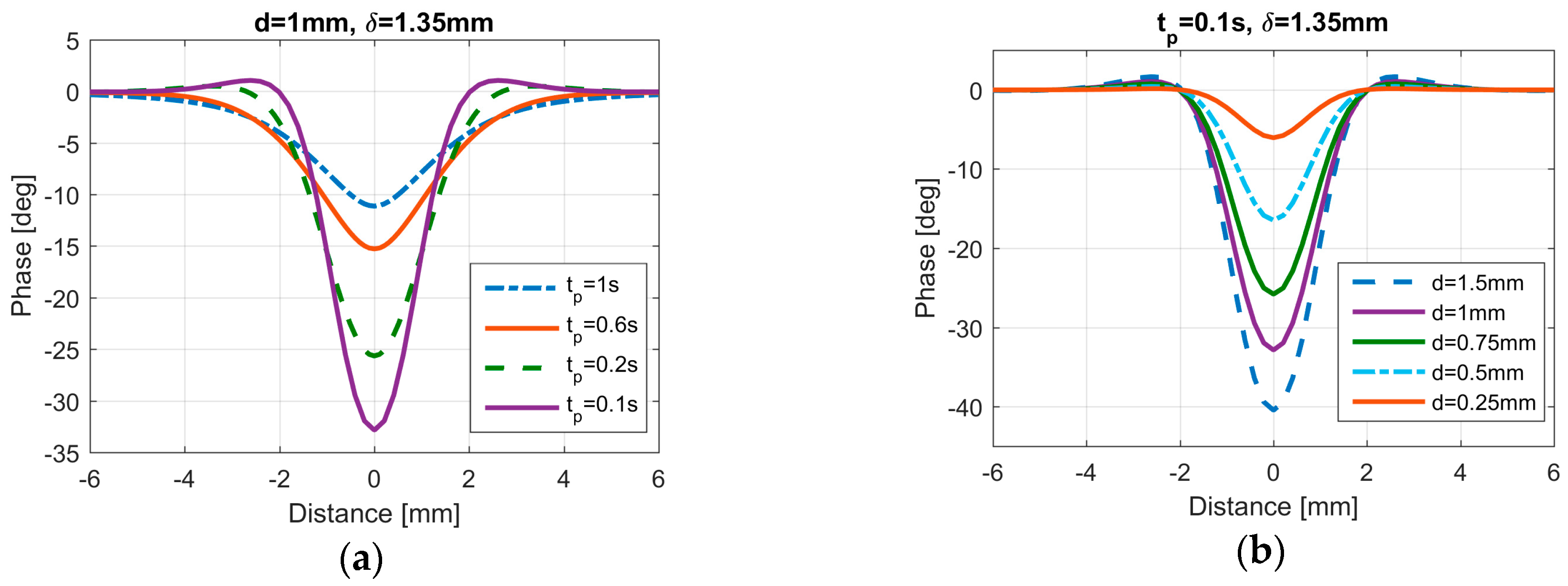
The heat becomes trapped in the corner with the smaller angle, as shown in Figure 12. From the other corner, which has an angle larger than 90° to the surface, the heat flows away much more quickly, resulting in an asymmetrical temperature distribution. As the phase value is a good measure for the heat flow rate, it is lower in the region with heat accumulation than that for a vertical crack. On the other side of the crack, which has a larger heat flow, the phase is higher than that for a vertical crack, so the phase distribution is asymmetrical (Figure 13). With a longer heating pulse, the heat flows away faster from the crack position, so the asymmetrical distribution decreases, and the difference between both sides becomes negligible. As shown earlier, dth/2 is approximately the distance where the phase value is at its minimum. In Figure 12, for both cases, the distance dth/2 is marked. In Figure 12a, this position (dth/2 = 1.08 mm) is close to the crack, so it has a strong influence. However, after a 1 s heat pulse (dth/2 = 3.4 mm, see Figure 12b), it is far away from the crack, and the temperature distribution and heat flow on both sides of the crack become very similar.
Figure 13a compares the phase distribution after different heating pulse durations for the same crack. For the short heating pulse, the phase distribution is strongly asymmetrical, but with longer pulses, and the difference between both sides diminishes. For comparison in Figure 13b for the same pulse durations, the phase for the vertical crack is shown. With longer heating, the phase around the inclined crack becomes almost symmetrical, but the phase value at the crack position is higher than that for a vertical crack with the same depth.
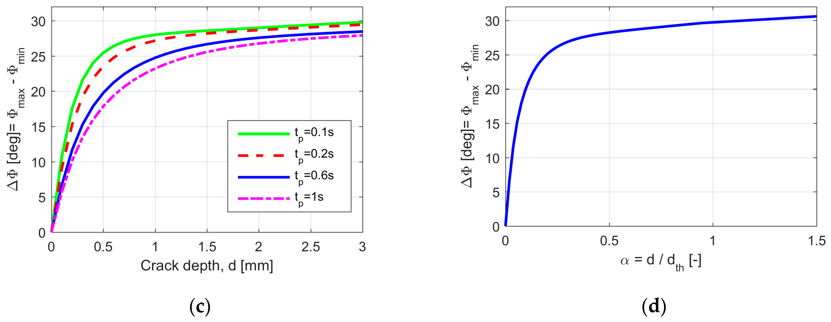
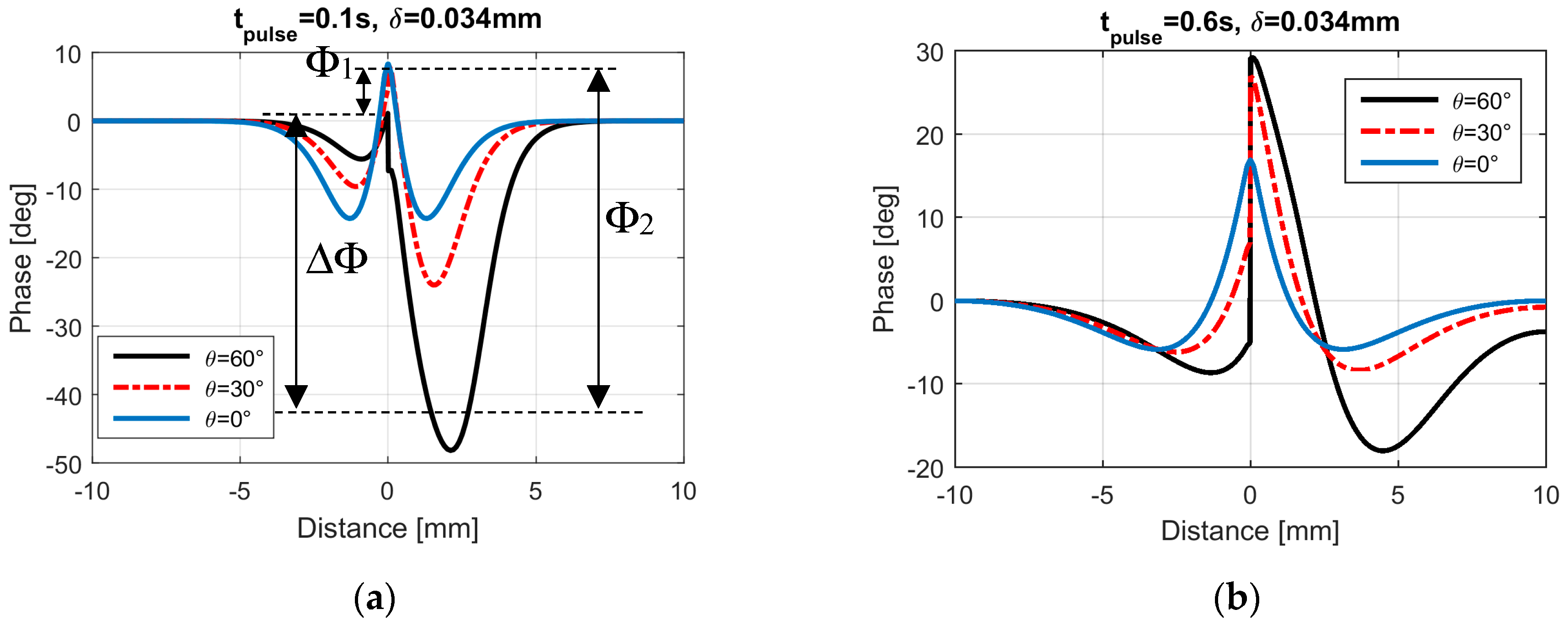
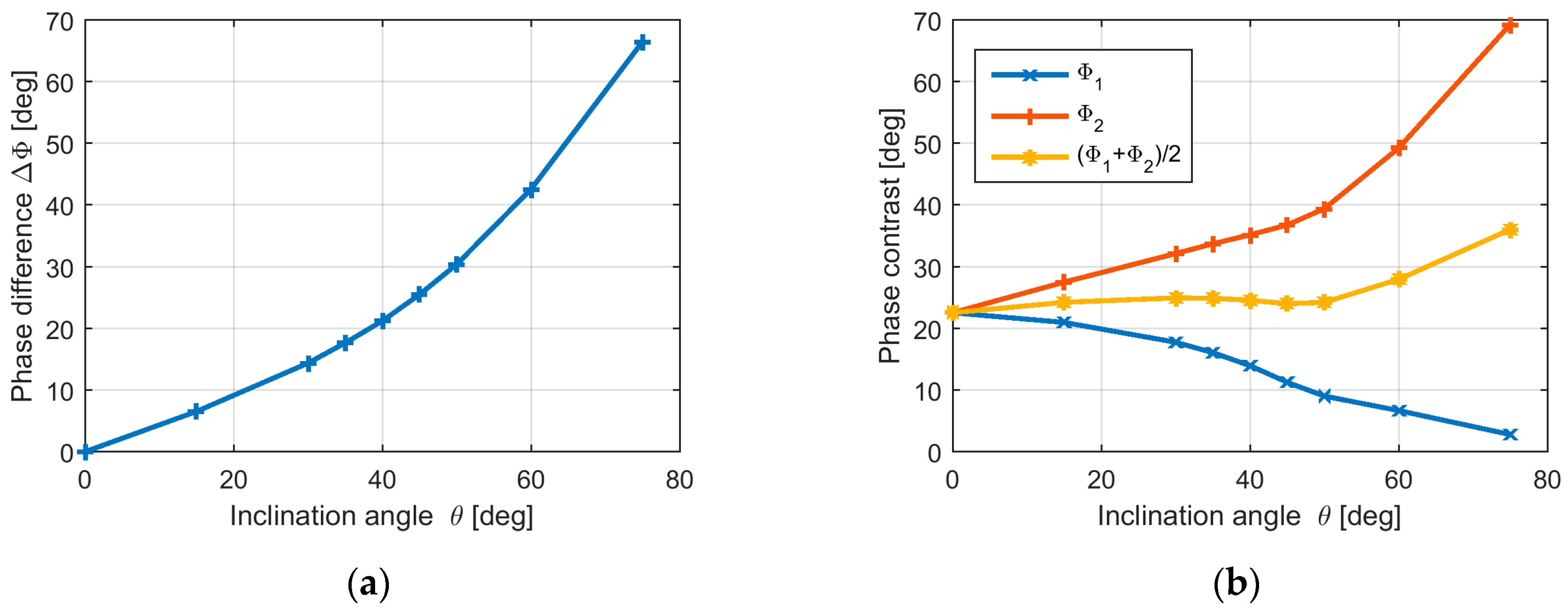
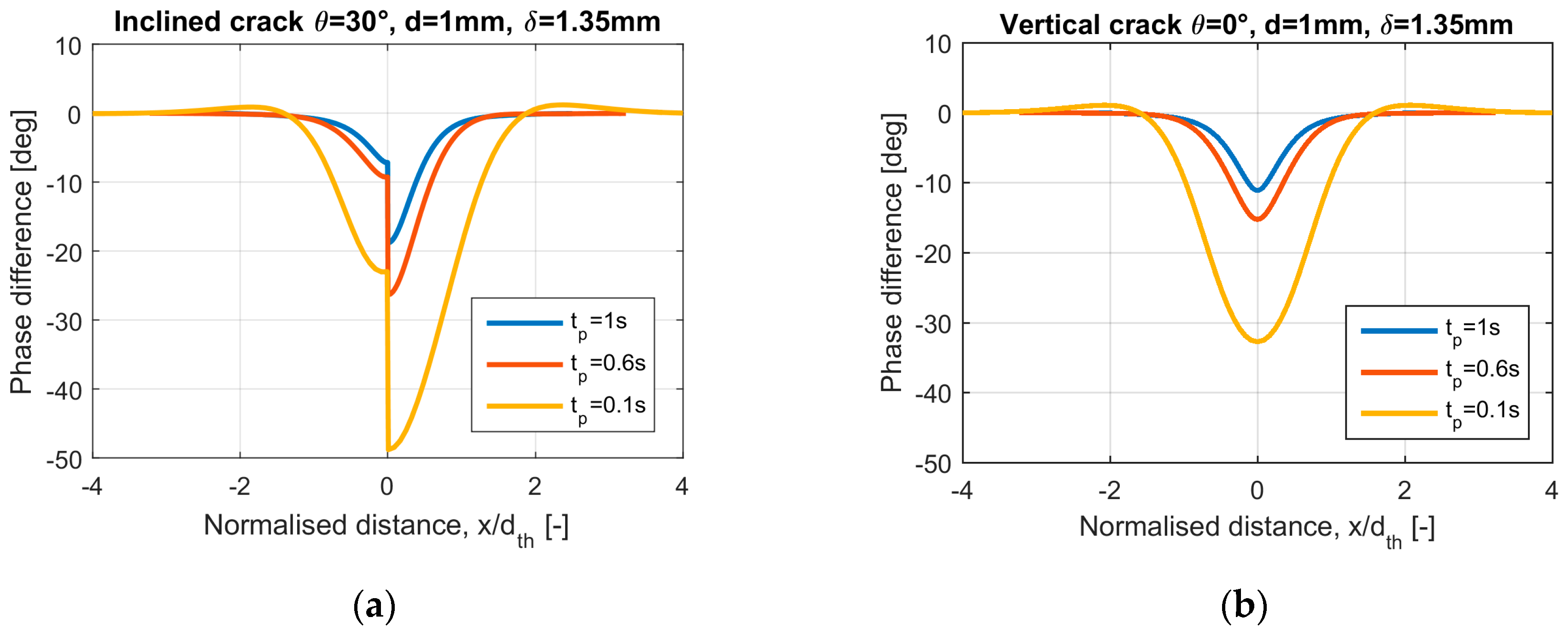
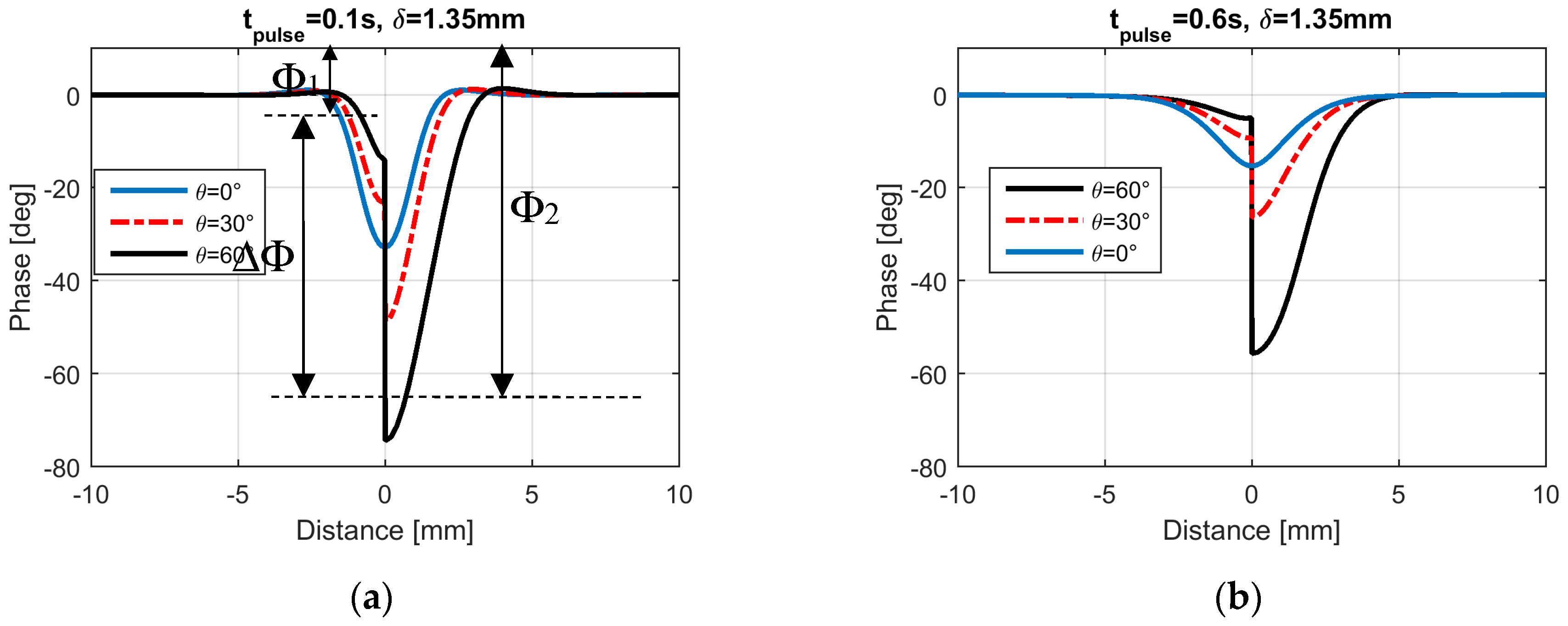
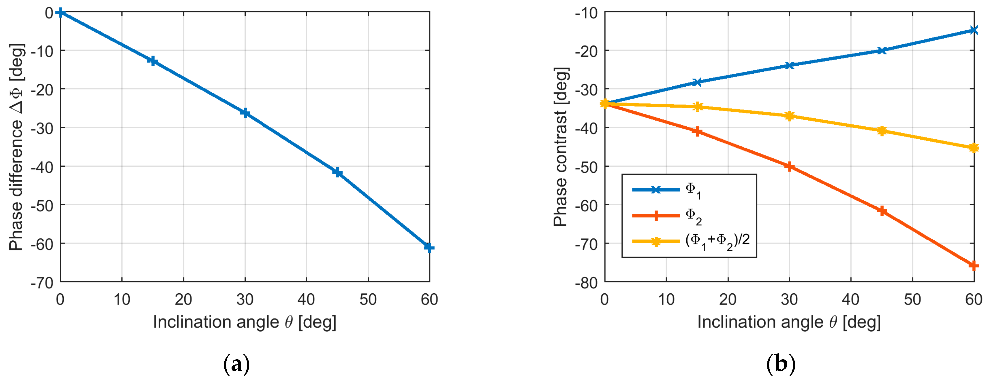
The larger the inclination angle θ, the longer the heat is trapped in the corner of the small angle, and the temperature and the phase distribution become strongly asymmetrical. Figure 14 demonstrates this behavior for different inclination angles. The difference between the phase minima of both sides ΔΦ is a measure for the asymmetry in the phase distribution. Figure 14a shows the phase for the short heating pulse of 0.1 s for three different angles. In Figure 15a, the dependency of ΔΦ on the inclination angle θ is plotted. The phase contrast on the left side (Φ1) is smaller for large inclination angles, as the heat can flow away without almost any obstacles (Figure 15b). On the other side of the crack, Φ2 increases with the θ values. For a short heating pulse of 0.1 s, the mean value of these two is close to the phase contrast of the vertical crack [23,26] (Figure 15b).
However, this is only valid for short heating pulses. As shown in Figure 12 and Figure 13a, the asymmetry in the phase decreases as pulse duration increases. Figure 14b shows the phase for the same three cracks in Figure 14a, but for a longer heating pulse. Even if there is less asymmetry, the phase at the crack position is larger than that for the vertical crack, so the depth of the crack can be overestimated.
Based on these results, a short heating pulse is recommended. Furthermore, the phase difference between both sides provides information about the inclination angle of the crack and the mean phase contrast regarding its depth [23].
6. Experimental Results for Inclined Cracks in Ferro-Magnetic Steel
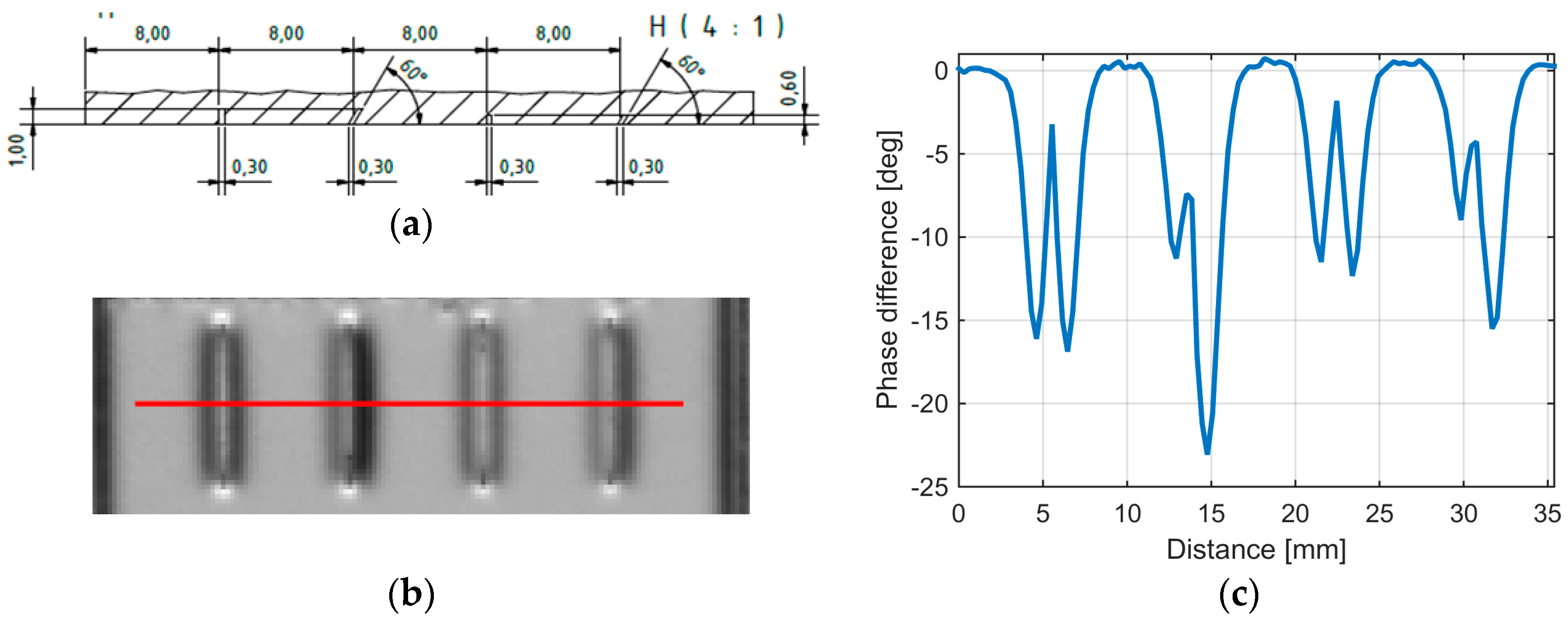
For experimental investigations of cracks with defined depths and inclination angle, two ferro-magnetic steel samples with artificial defects were produced. The first one is a laser-sintered sample, where four artificial cracks with a length of 10 mm and depths of 1 mm and 0.6 mm (see Figure 16a) were manufactured [23]. The cracks had a width of 0.3 mm and thus were closer in appearance to a kind of notch instead of natural cracks, which usually have a width of only a couple of µm (see Figure 8a and Figure 11a). However, these artificial cracks or notches also showed results that are very similar to those presented by the simulation predictions.
Two of the cracks of the sintered sample were vertical and two of them had an inclination angle of θ = 30°. Figure 16b,c show the phase image after a 0.1 s heating pulse and a profile through the phase image. As this is in good agreement with the previous sections, one can observe
- that the deeper crack has a higher phase contrast than the shallower one;
- that the phase profile of the inclined cracks is asymmetric and the mean value of the phase minima at the left and right sides is almost equal to the minimum phase of the vertical crack.
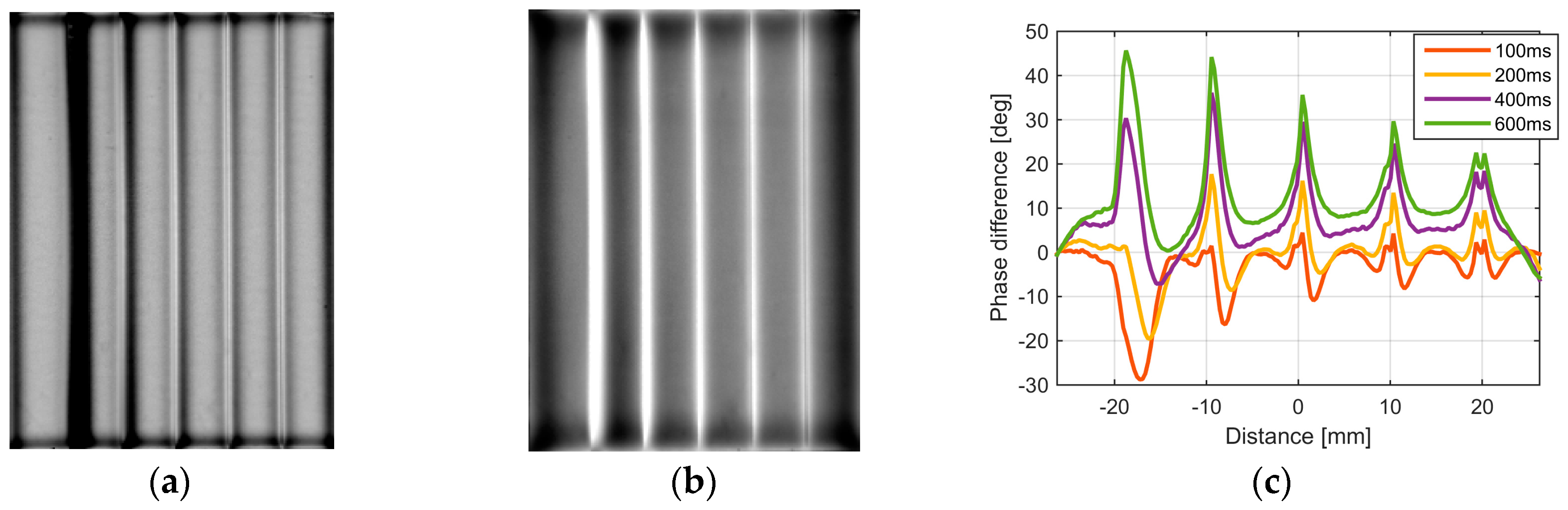
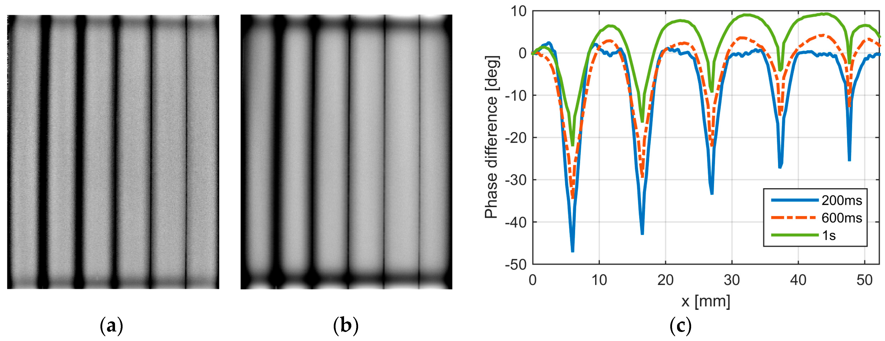
The second sample is a 30 × 60 × 80 mm³ ferro-magnetic steel sample, where five defects were cut with the EDM technique (electro-discharge machining). Each of them had a depth of 1 mm, but the inclination angles varied from 75° up to 0°. Figure 17 shows the phase images after 0.1 s and 0.6 s heating pulses and different phase profiles. Like the simulation results, also shown in Figure 14, the following can be observed:
- For a short heating pulse (100 and 200 ms), the phase is asymmetric, and the wider the inclination angle is, the greater the difference is between the phase at the left and right sides of the crack.
- For longer pulses (400 and 600 ms), asymmetry decreases.
- The larger the inclination angle, the higher the phase value at the crack position.
It is important to note that, in both of the samples with artificial defects, the defect width was about 0.3 mm, which is much larger than the width of the natural cracks that are usually not visible at the surface. It is very difficult to manufacture artificial defects with a given depth and angle, but with a very small width. Even so, these artificial samples can be used well as test objects to investigate different behaviors.
7. Vertical Cracks with Large Eddy Current Penetration Depth
In the previous sections, an eddy current penetration depth was assumed, which is small compared to the crack depth. Since, for non-magnetic materials, the penetration depth is significantly larger, this assumption is no longer valid. For the simulation of this scenario, the simu.2 model can be used as it also considers the distribution of the eddy current and the Joule heating (see Table 2). If the crack is vertical, which is listed as “Case 2” in Table 2, then the eddy current is deviated by the crack and will not flow close to the crack corner (Figure 18a) [27,28]. Therefore, the Joule heating in this region is less than that at the sound surface (Figure 18b). A hot spot occurs at the tip of the crack, but this is inside the sample and not visible at the surface.
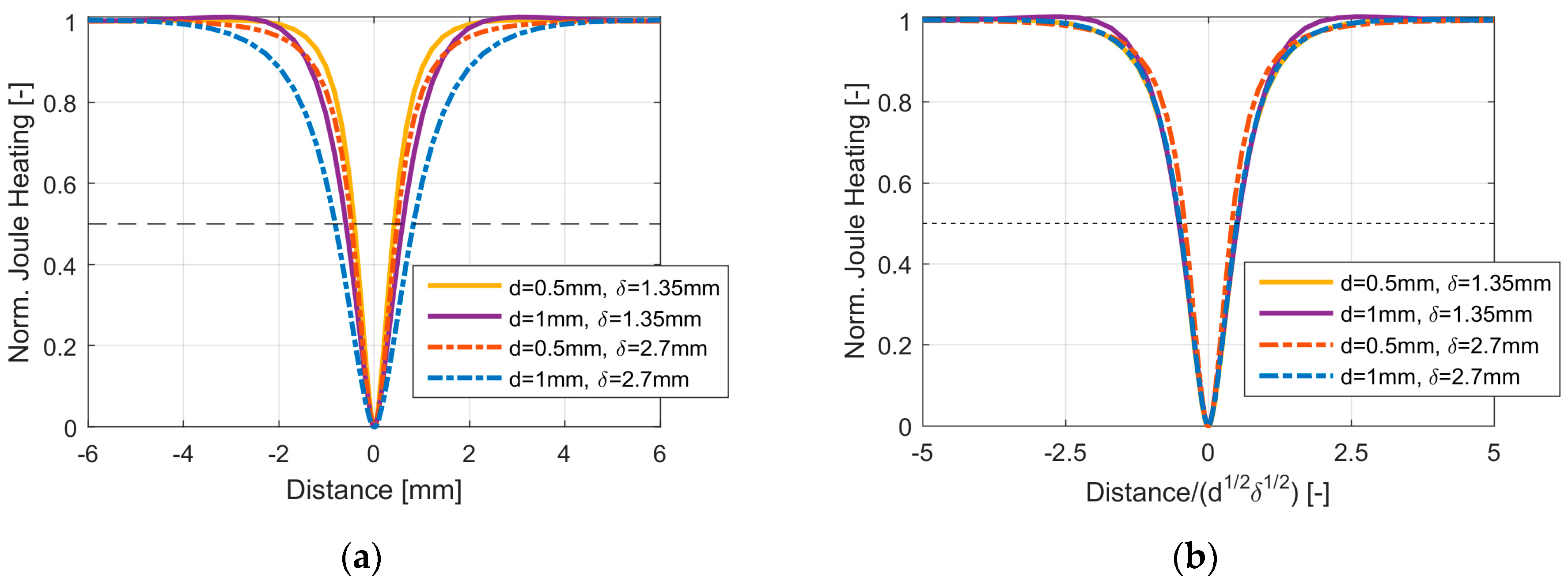
In Figure 19, the Joule heating at the surface, normalized between 0 and 1, is plotted and compared for different crack and penetration depths. The deeper the crack, the broader the region around the crack, where the Joule heating is lower than it is at the sound surface. This is also valid for the penetration depth: the larger δ is, the broader the region where the eddy current is pushed inside from the surface into the inner part of the material. Normalizing the distance to , the curves become almost identical (Figure 19b). Introducing β for the ratio crack depth to penetration depth
the full-width-half-maximum (FWHM) of the curves is approximately
As the Joule heating at the surface in the corner of the crack is low, the temperature in this region immediately after the heat is switched on is less than that at the sound surface (Figure 20a). With increasing time, the heat diffusion equalizes this difference, the heat flows into the corners, and the temperature becomes more homogeneous (Figure 20b).
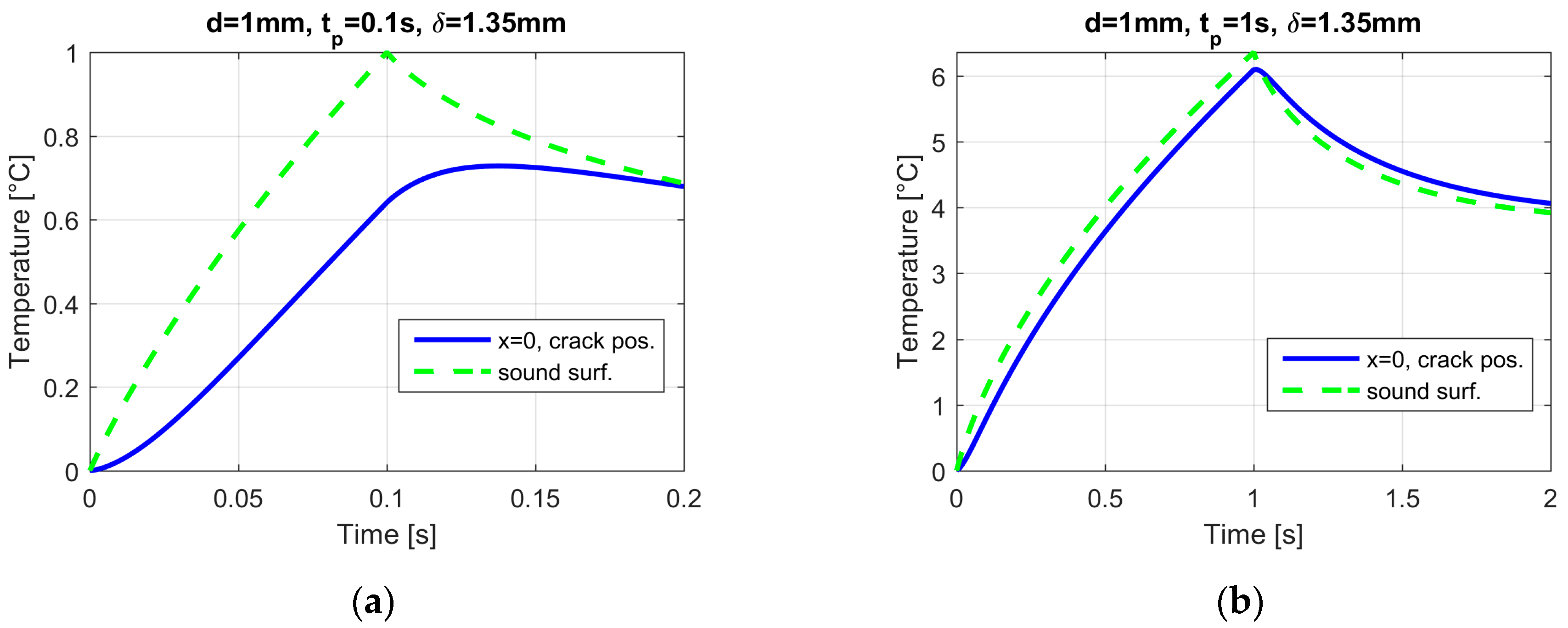
Figure 21 compares the temperature curves at the crack position and at the sound surface. If the heating pulse is short (Figure 21a), then the crack is significantly cooler than the sound surface, as there is less Joule heating in this region. It is also observed that the temperature at the crack reaches its maximum later than the heating was switched off. Even if there is no longer any heating, due to the heat diffusion, the heat flows further into this cooler region and increases the temperature. If the heating pulse is long (Figure 21b), then, with increasing time, the difference between the temperature at the crack position and at the sound surface becomes negligibly small.
Calculating the phase from the temperature functions, the area around the crack has lower values than that at the sound surface. In Figure 22a, the phase distribution for different pulse heating durations is plotted. The shorter the pulse, the larger the phase difference due to the crack.
The deeper the crack, the more the eddy currents deviate into the material, so the phase difference increases as crack depth increases (Figure 22b). Figure 23a shows the relative temperature contrast for different penetration depths that were simulated for a crack with a depth of 1 mm. Three curves were calculated for ferro-magnetic steel (dash-dot lines) and the other three were for non-magnetic steel (solid lines). To be able to compare different materials, the abscissa is normalized to
at which time the heat flows into a distance of d due to diffusion. In Figure 23a, it can be observed that
- as penetration depth increases, the relative contrast becomes negative as the temperature at the crack position becomes lower than that at the sound surface;
- with increasing time, due to heat diffusion, the relative contrast decreases in absolute value.
In Figure 23, the analytical calculation results of Equation (5) are also plotted with a dashed line relating to a penetration depth of δ = 0 mm.
Assuming a detection limit of +0.1 and −0.1 for the relative temperature contrast, a defect with a 1 mm depth can be detected with a positive CR if the penetration depth is small compared to crack depth. Another possibility for detection is a negative CR if the penetration depth is comparable with crack depth. However, in this second case, time duration of the possible observation is limited due to the equalization process of heat diffusion.
In Figure 23b, phase differences are depicted for the same cases, and the temperature contrast is shown in Figure 23a. Generally, a negative temperature contrast results in a negative phase difference, and a positive CR causes a positive phase difference. However, as the phase calculation considers the whole heating and cool-down duration, the detection of a crack from the phase is possible for a longer pulse duration than that from the temperature. For example, when δ = 1 mm, a crack with a depth of 1 mm in non-magnetic steel in the temperature contrast can be detected up to t = 5 tdth ~0.31 s, and in the phase image up to t = 15 tdth ~0.93 s, assuming a detection limit of 10°.
As has been shown, the deeper the crack, the larger the effect it has on the eddy current distribution; consequently, it causes a larger phase difference in absolute value. Figure 24a compares the phase values for two penetration depths if the crack is 1 mm and 0.5 mm deep. δ = 0.1 mm (dash-dot line) was calculated for ferro-magnetic steel, and δ = 0.5 mm (solid line) for non-magnetic steel. It was observed that the phase values of the smaller crack were closer to zero, so are more difficult to detect.
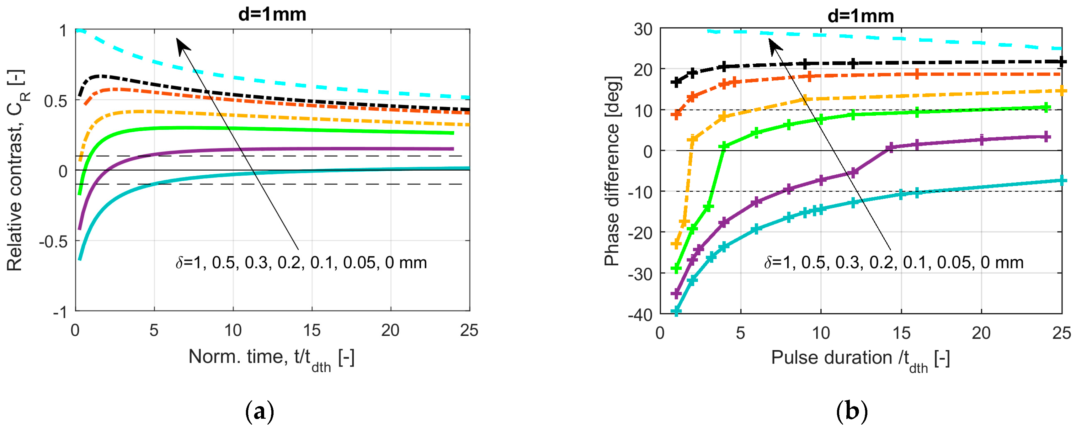
We defined two ratios α (Equation (6)) and β (Equation (8)) that mainly determine the phase distribution. Comparing two cracks with a depth of d and d/2, all distances, including the penetration depth and the diffusion length, have to be reduced to half to obtain the same phase distribution. To reduce the penetration depth to half, a fourfold higher excitation frequency is required; to reduce the diffusion length to half requires a reduction in the pulse duration to one-fourth. Thus, the phase distribution around both cracks becomes the same; however, for the smaller one, the distances are proportionally half of the larger one. This proportionality allows a normalized plotting of the phase contrast (Figure 24b). This diagram is valid for each crack depth, penetration depth, and pulse duration, based on the assumption that the crack is vertical and no electrical flow between the crack sides is possible.
Figure 24b also shows the result of the analytical calculation (dashed line) corresponding to β = ∞. This curve is the same one as the one shown in Figure 6d, but instead of α is now 1/α logarithmically plotted at the abscissa.
One important question is how different crack depths can be distinguished by a given pulse duration. In Figure 25a, two different penetration depths (δ = 0.034 mm and f = 200 kHz for ferro-magnetic steel; δ = 1 mm and f = 361 kHz for non-magnetic steel) are compared for three different pulse durations. Additionally, the analytically calculated curves with δ = 0 mm as per Figure 6b are shown. The following can be observed:
- For small penetration depths (e.g., δ = 0.034 mm), the positive phase difference increases with the crack depth and it tends toward a maximum. The curves for the different pulse durations are similar.
- For large penetration depths (e.g., δ = 1 mm), the phase difference increases in the negative direction as crack depth increases, and the shorter the pulse duration is, the greater the phase value becomes.
These curves are shown in Figure 25b as normalized curves, depending on both ratios. The curves are parametrized with β/α = d/δ.
8. Experimental Results for Vertical Cracks in Non-Magnetic Steel
In an AISI 304 non-magnetic steel sample with a size of 30 × 60 × 80 mm³, five artificial cracks were cut with the EDM technique. The cracks had different depths in the range of 0.5–2 mm. The measurement circumstances were the same as described in Section 4. The material parameters according to the literature are listed in Table 1, where the eddy current penetration depth is about 1.35 mm.
Figure 26 shows the results for this sample, which are in good agreement with the numerically simulated ones of the previous section:
- The cracks are well visible due to the lower phase values around them when compared to the sound surface.
- The deeper the crack is, the larger its phase difference in absolute value is.
- As heating pulse increases, the absolute value of the phase difference decreases.
- The shorter the pulse is, the sharper the phase signal is around the crack. As pulse duration increases, the thermal diffusion length also increases, resulting in a broadening of the signal around the crack position.
In Figure 27, the results are shown for a titanium wire with a 20 mm diameter. The experimental setup was also the same as that described in Section 4. With a 200 kHz excitation frequency, the penetration depth is about 0.8 mm. The results are in good agreement with the calculated ones of the previous section:
9. Inclined Cracks with Large Eddy Current Penetration Depth
In Case 4 of Table 2, the crack is inclined and the penetration depth is comparable with the crack depth. Simulations were carried out with the model simu.2, and the results are presented in Figure 28 and Figure 29.
The results are a combination of the previous observations, but in a more complex manner. The phase profiles are asymmetrical (Figure 30a) for the same reasons as those explained in Section 5. As pulse duration increases, the asymmetry and the phase values decrease.
The wider the inclination angle is, the greater the phase difference ΔΦ between both sides of the crack becomes (Figure 31a and Figure 32a). If the pulse is longer (Figure 31b), then the asymmetry and the phase value will be less, also for higher inclination angles.
The mean value of Φ1 and Φ2 for short pulses presents less dependency on the inclination angle (see Figure 32b) and can be used by measurements for the estimation of the crack depth.
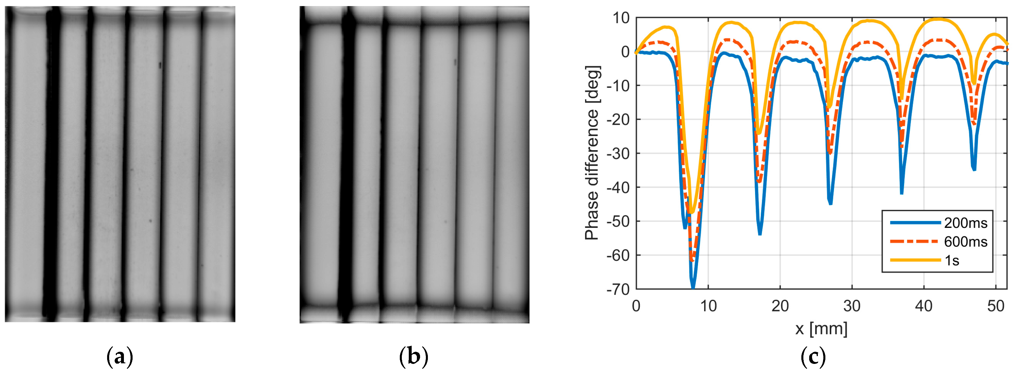
10. Experimental Results for Inclined Cracks in Non-Magnetic Steel
A similar sample, as shown in Section 6, was also manufactured from non-magnetic steel. All artificial cracks had a depth of 1 mm, and the inclination angles changed in the same manner as for the ferro-magnetic sample. The experimental setup was the same as that described previously (see Figure 33a–c).
From these results, similar conclusions can be made as in the previous sections:
- With longer pulses, the phase contrast decreases;
- For larger inclination angles, the phase profile is asymmetrical and has a higher value than that for vertical cracks.
11. Conclusions and Summary
It has been shown that induction thermography can be used to detect surface cracks and to estimate crack depth. It is possible to use it for ferro-magnetic and for non-magnetic materials, but the measurement circumstances such as excitation frequency and pulse length have to be adapted to the material.
If the crack is perpendicular to the surface, then two ratios determine the results. One of them is the ratio of the crack depth to the penetration depth of the eddy current, and the second one is the ratio of the crack depth to the thermal diffusion length. Using finite element simulations, the eddy current and temperature distributions were calculated and phase images determined. The calculated normalized phase difference curves (Figure 24b and Figure 25b) can be applied for any metal, and provide a good approximation of the crack depth under given measurement parameters.
The situation is more complex for inclined cracks. The simulations and measured results show that short pulses produce an asymmetrical phase distribution, from which not only the crack depth but also the inclination angle can be estimated. In specific cases, it can be very useful to carry out the measurements with several pulse lengths and combine their results to more precisely estimate the crack depth.
In this paper, the influence of the measurement conditions, the material parameters, the crack depth, and its inclination angle on the temperature and phase contrast were investigated to provide a guide for optimizing the experimental setup. The goal is not only to detect a surface crack but also to be able to estimate its depth.
Additionally, for the detectability of the cracks, the signal-to-noise ratio (SNR) plays a very important role. If the heating power is low, especially for non-magnetic materials with a short heating pulse duration, then the noise may become significant and hamper detection. Further investigations are in progress to investigate the influence of the SNR on detectability also by applying multiple pulses as a lock-in technique.
In this study, cracks that have a length of at least 10 mm at the surface were investigated. For shorter cracks, the hot spots around their crack tips dominate the infrared images. Further 3D numerical simulations and experiments are planned to investigate this case.
Acknowledgments
Financial support by the Austrian Federal Government (in particular from Bundesministerium für Verkehr, Innovation und Technologie, and Bundesministerium für Wissenschaft, Forschung und Wirtschaft) represented by Österreichische Forschungsförderungsgesellschaft mbH and the Styrian and the Tyrolean Provincial Government, represented by Steirische Wirtschaftsförderungsgesellschaft mbH and Standortagentur Tirol, within the framework of the COMET Funding Program is gratefully acknowledged.
Author Contributions
The author claims to have developed all the methods presented here.
Conflicts of Interest
The author declares no conflict of interest.
References
- Lucía, O.; Maussion, P.; Dede, E.; Burdío, J.M. Induction Heating Technology and its Applications: Past Developments, Current Technology, and Future Challenges. IEEE Trans. Ind. Electron. 2014, 61, 2509–2520. [Google Scholar] [CrossRef] [Green Version]
- Kremer, K.J.; Kaiser, W.; Möller, P. Das Therm-O-Matic-Verfahren—Ein neuartiges Verfahren für die Online-prüfung von Stahlerzeugnissen auf Oberflächenfehler. Stahl und Eisen 1985, 105, 39–44. [Google Scholar]
- Maldague, X. Infrared and Thermal Testing, Nondestructive Testing Handbook, Vol. 3. ASNT, Columbus, OH. 2001. Available online: http://www.asnt.org (accessed on 1 January 2018).
- Riegert, G.; Zweschper, T.; Busse, G. Lockin thermography with eddy current excitation. Quant. InfraRed Thermogr. J. 2004, 1, 21–32. [Google Scholar] [CrossRef]
- Riegert, G.; Gleiter, A.; Busse, G. Potential and limitations of eddy current lockin-thermography. Defense Secur. Symp. 2006, 6205. [Google Scholar] [CrossRef]
- Oswald-Tranta, B. Thermoinductive investigations of magnetic materials for surface cracks. Quant. InfraRed Thermogr. J. 2004, 1, 33–46. [Google Scholar] [CrossRef]
- Vrana, J.; Goldammer, M.; Baumann, J.; Rothenfusser, M.; Arnold, W. Mechanism and models for crack detection with induction thermography. AIP Conf. Proc. 2008, 1706, 475–482. [Google Scholar]
- Wilson, J.; Tian, G.Y.; Abidin, I.Z.; Yang, S.; Almond, D. Modeling and evaluation of eddy current stimulated thermography. J. Nondestr. Test. Eval. 2010, 25, 205–218. [Google Scholar] [CrossRef]
- Netzelmann, U.; Walle, G. Induction Thermography as a Tool for Reliable Detection of Surface Defects in Forged Components. In Proceedings of the 17th World Conference on Non Destructive Testing, Shanghai, China, 25–28 October 2008. [Google Scholar]
- Oswald-Tranta, B.; Sorger, M. Localizing surface cracks with inductive thermographical inspection: From measurement to image processing. Quant. InfraRed Thermogr. J. 2011, 8, 149–164. [Google Scholar] [CrossRef]
- Netzelmann, U.; Walle, G.; Ehlen, A.; Lugin, S.; Finckbohner, M.; Bessert, S. NDT of Railway Components Using Induction Thermography. AIP Conf. Proc. 2016, 1706, 150001. [Google Scholar]
- Wilson, J.; Tian, G.; Mukriz, I.; Almond, D. PEC Thermography for Imaging Multiple Cracks from Rolling Contact Fatigue. NDT E Int. 2011, 44, 505–512. [Google Scholar] [CrossRef]
- Abidin, I.Z.; Tian, G.Y.; Wilson, J.; Yang, S.; Almond, D. Quantitative evaluation of angular defects by pulsed eddy current thermography. NDT E Int. 2010, 43, 537–546. [Google Scholar] [CrossRef]
- Wally, G.; Oswald-Tranta, B. The influence of crack shapes and geometries on the results of the thermo-inductive crack detection. In Proceedings of the SPIE Thermosense XXIX, Orlando, FL, USA, 9–12 April 2007. [Google Scholar]
- Srajbr, C. Induction Excited Thermography in Industrial Applications. In Proceedings of the 19th World Conference on Non-Destructive Testing, Munich, Germany, 13–17 June 2016. [Google Scholar]
- Netzelmann, U.; Walle, G.; Lugin, S.; Ehlen, A.; Bessert, S.; Valeske, B. Induction thermography: Principle, applications and first steps towards standardization. Quant. InfraRed Thermogr. J. 2016, 13, 170–181. [Google Scholar] [CrossRef]
- DIN 54183:2018-02, Non-Destructive Testing-Thermographic Testing- Eddy-Current Excited Thermography. Available online: https://www.din.de (accessed on 1 January 2018).
- Oswald-Tranta, B. Time-resolved evaluation of inductive pulse heating measurements. Quant. InfraRed Thermogr. J. 2009, 6, 3–19. [Google Scholar] [CrossRef]
- Oswald-Tranta, B. Automated Thermographic Non-Destructive Testing. Habilitation, University of Leoben, Leoben, Austria, 2012. [Google Scholar]
- ANSYS, Inc. Available online: http://www.ansys.com (accessed on 1 January 2018).
- Bowler, N. Frequency dependence of relative permeability in steel. Rev. Prog. Quant. Nondestr. Eval. 2006, 25, 1269–1276. [Google Scholar]
- Jäckel, P.; Netzelmann, U. The influence of external magnetic fields on crack contrast in magnetic steel detected by induction thermography. Quant. InfraRed Thermogr. J. 2013, 10, 237–247. [Google Scholar] [CrossRef]
- Oswald-Tranta, B. Investigations for Determining Surface Crack Depth with Inductive Thermography. In Proceedings of the 19th World Conference on Non-Destructive Testing, Munich, Germany, 13–17 June 2016. [Google Scholar]
- Oswald-Tranta, B.; Wally, G. Thermo-inductive investigations of steel wires for surface cracks. In Proceedings of the SPIE Thermosense XXVII, Orlando, FL, USA, 28 March–1 April 2005. [Google Scholar]
- Seidel, M.W.; Zosch, A.; Seidel, C.; Hartel, K.; Grafe, F. Herstellung und Anwendung von Vergleichskörpern für die Schleifbrandprüfung und die Rissprüfung. In Proceedings of the Seminar des FA Oberflächenrissprüfung, Kassel, Germany, 14–15 October 2015. [Google Scholar]
- Oswald-Tranta, B. Untersuchungen zur Bestimmung der Risstiefe mit induktiver Thermografie. In Proceedings of the Thermographie-Kolloquium, Stuttgart, Germany, 1–2 October 2015. [Google Scholar]
- Oswald-Tranta, B.; Wally, G. Thermo-inductive surface crack detection in metallic materials. In Proceedings of the 9th European Conference on NDT, Berlin, Germany, 25–29 September 2006. [Google Scholar]
- Oswald-Tranta, B. Thermo-inductive Crack Detection. J. Nondestr. Test. Eval. 2007, 22, 137–153. [Google Scholar] [CrossRef]
Figure 1.
Simulation model (simu.2) results shown close-up to a vertical surface crack with a depth of 1 mm. Material: ferro-magnetic steel, properties are listed in Table 1. Excitation frequency is 200 kHz. (a) Joule-heating. (b) Temperature distribution after a 0.1 s heating duration.
Figure 1.
Simulation model (simu.2) results shown close-up to a vertical surface crack with a depth of 1 mm. Material: ferro-magnetic steel, properties are listed in Table 1. Excitation frequency is 200 kHz. (a) Joule-heating. (b) Temperature distribution after a 0.1 s heating duration.

Figure 2.
Temperature increase at the crack position (x = 0), at the sound surface far away from the defect, and at the position x = dth/2, compared with the three models for the same case as shown in Figure 1.
Figure 2.
Temperature increase at the crack position (x = 0), at the sound surface far away from the defect, and at the position x = dth/2, compared with the three models for the same case as shown in Figure 1.

Figure 3.
Temperature (a) and phase difference (b) around a crack calculated with the three models for the same case as in Figure 1 and in Figure 2.
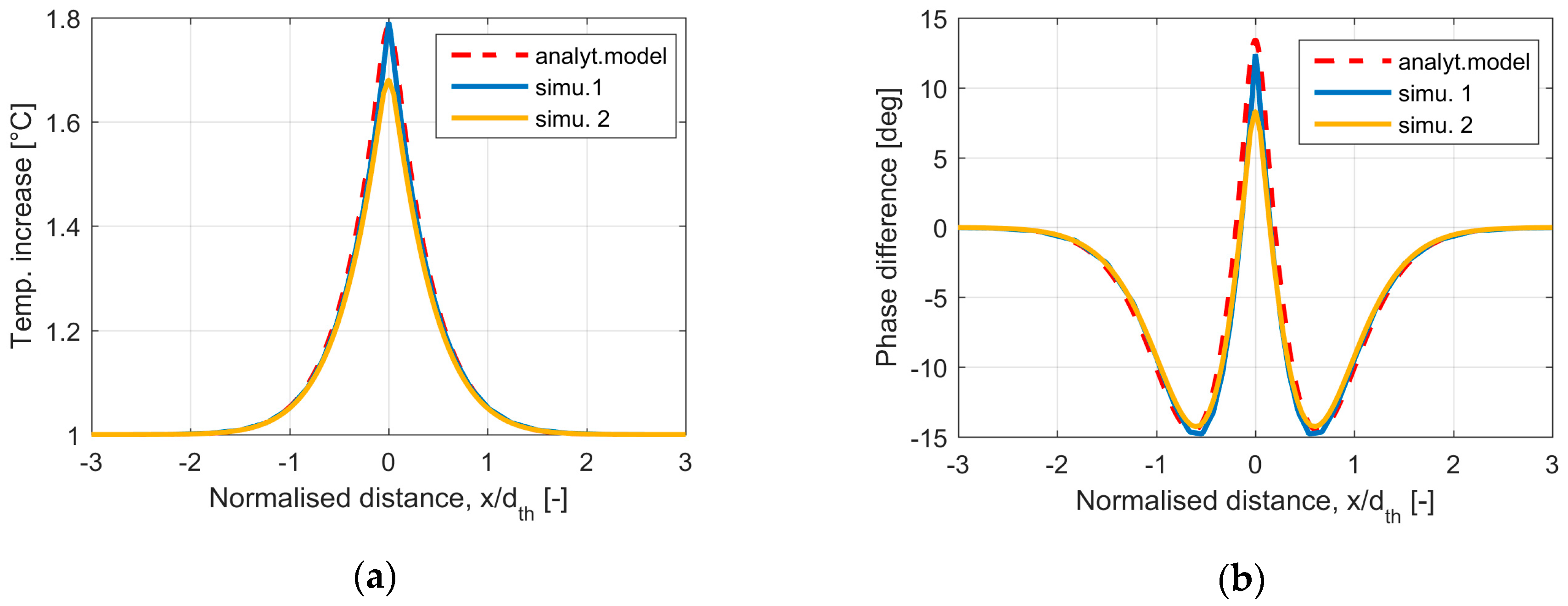
Figure 4.
Temperature (a) and phase difference (b) around a crack (d = 1 mm) as shown in previous figures, calculated for different pulse lengths using the simu.2 model.
Figure 4.
Temperature (a) and phase difference (b) around a crack (d = 1 mm) as shown in previous figures, calculated for different pulse lengths using the simu.2 model.

Figure 5.
Temperature (a) and phase difference (b) around cracks with different depths after a 0.1 s pulse duration.
Figure 5.
Temperature (a) and phase difference (b) around cracks with different depths after a 0.1 s pulse duration.
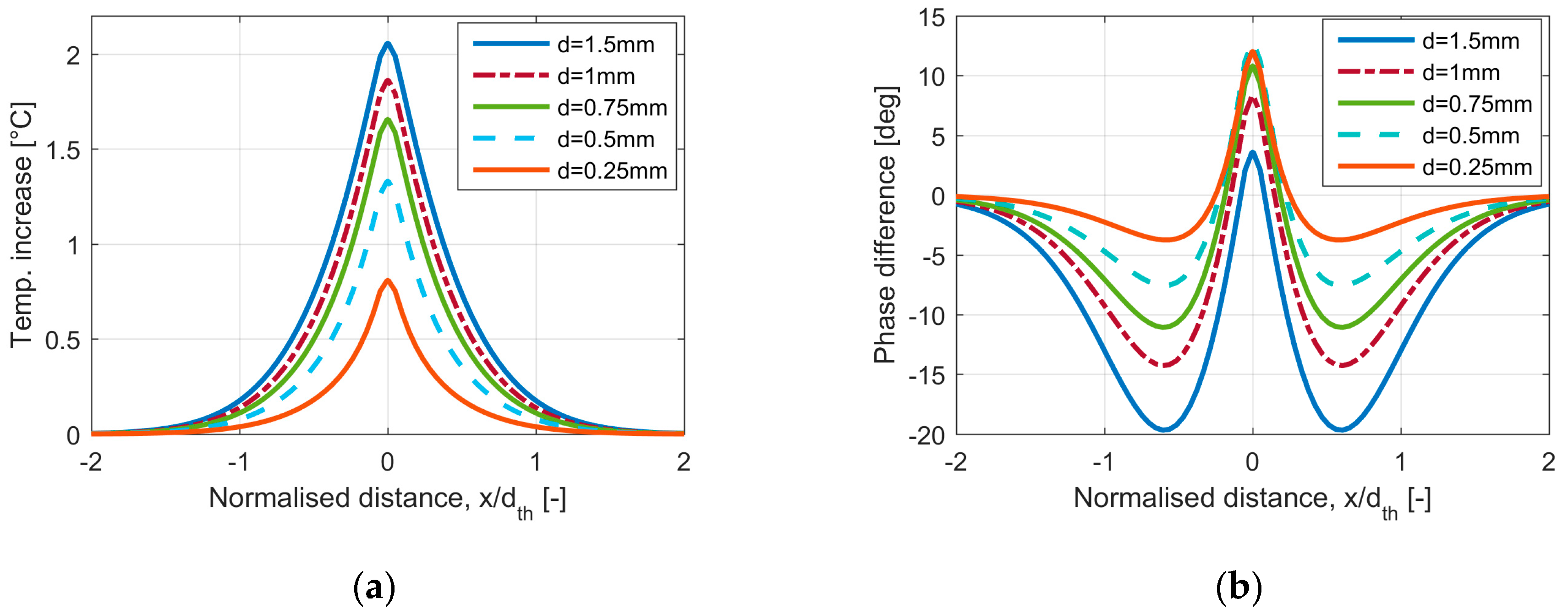
Figure 6.
Temperature (a) and phase difference (c) depending on crack depth; relative temperature contrast (b) and phase difference (d) depending on the relative crack depth α, calculated with Equations (4)–(7) for ferro-magnetic steel material parameters.
Figure 6.
Temperature (a) and phase difference (c) depending on crack depth; relative temperature contrast (b) and phase difference (d) depending on the relative crack depth α, calculated with Equations (4)–(7) for ferro-magnetic steel material parameters.


Figure 7.
Helmholtz coil with a wire, for which the results are shown in Figure 8.
Figure 7.
Helmholtz coil with a wire, for which the results are shown in Figure 8.
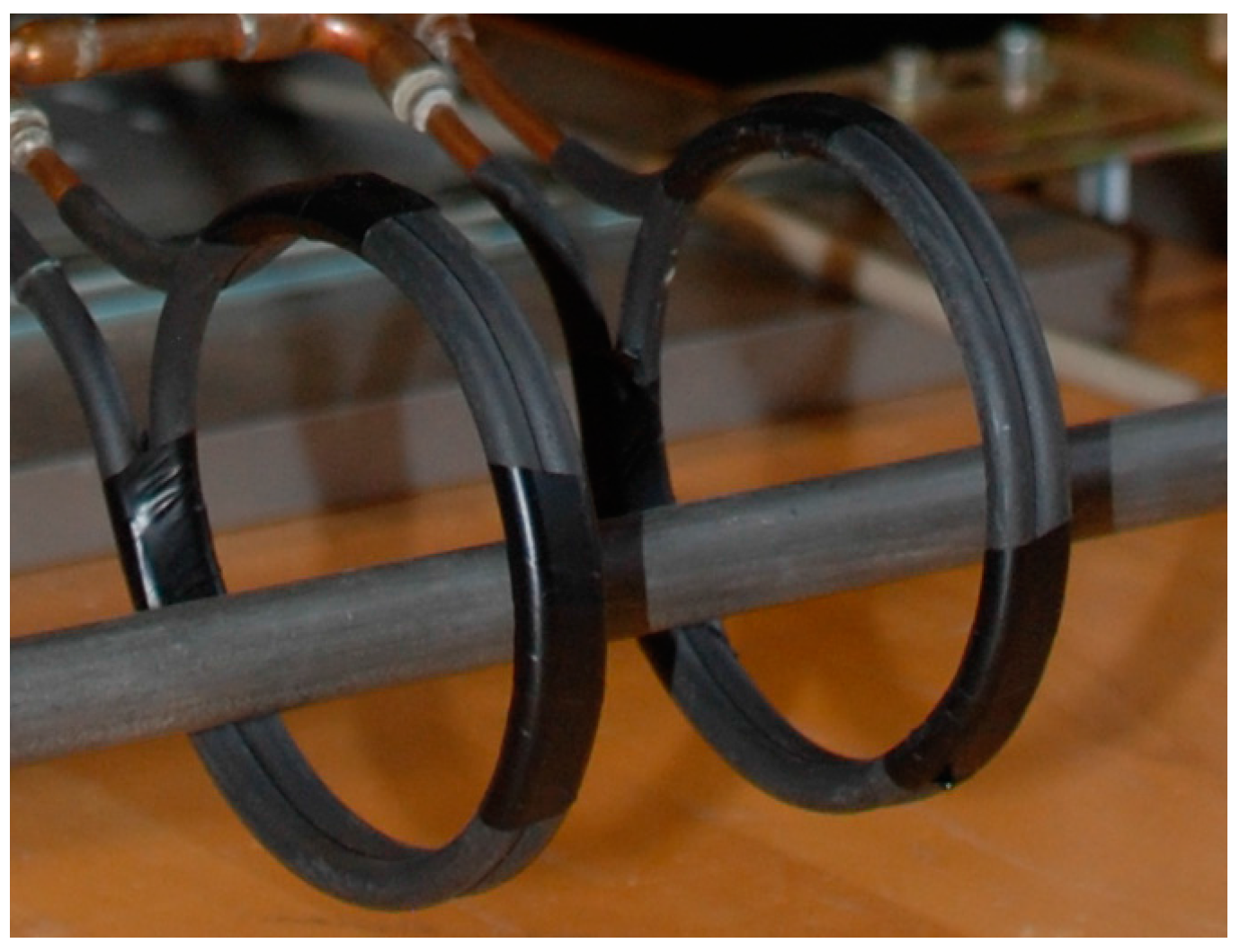
Figure 8.
Microscopic image through the wire (a), a phase image (b), and measured phase profiles compared with the analytically calculated phase (c).
Figure 8.
Microscopic image through the wire (a), a phase image (b), and measured phase profiles compared with the analytically calculated phase (c).

Figure 9.
(a) Phase image of a 12 mm long crack after a 0.1 s heating pulse at a ground surface; (b) the measured phase profile compared with the calculated one for a 1 mm depth.
Figure 9.
(a) Phase image of a 12 mm long crack after a 0.1 s heating pulse at a ground surface; (b) the measured phase profile compared with the calculated one for a 1 mm depth.
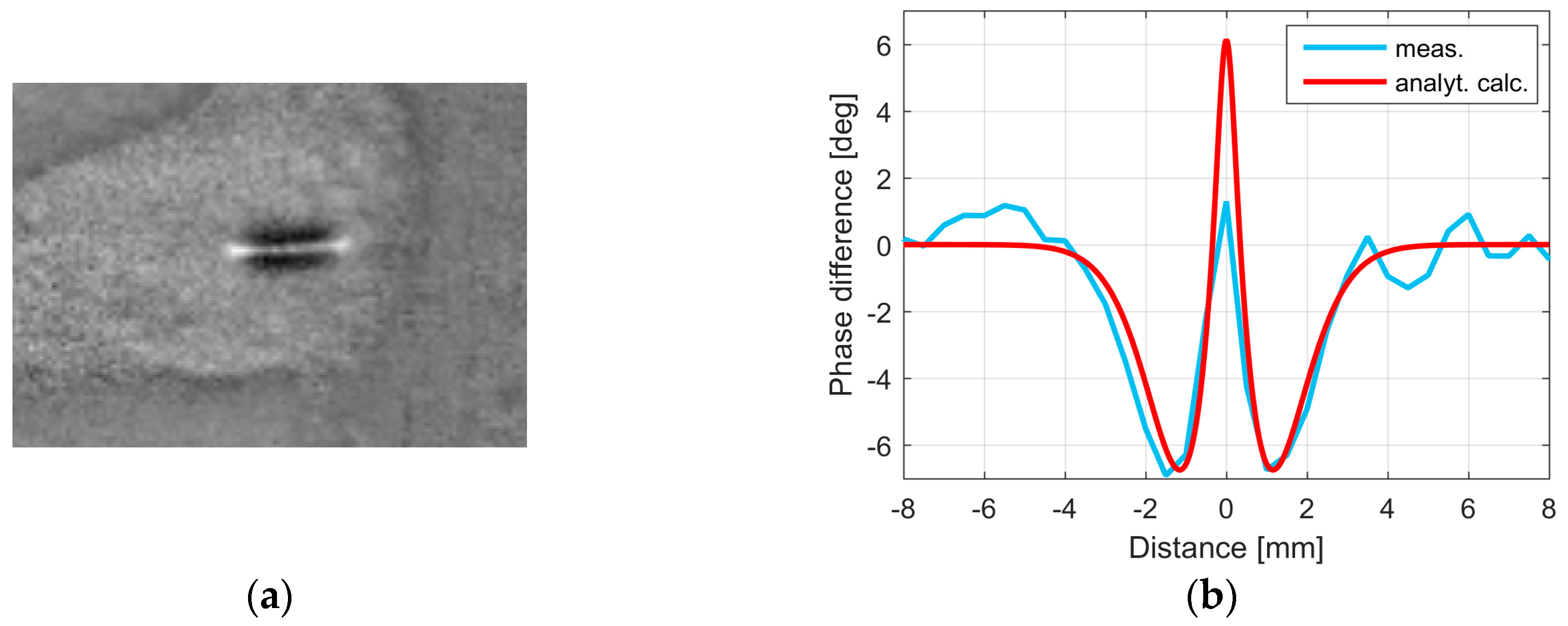
Figure 10.
(a) Phase images of two samples measured with a pulse duration of 0.1 s. The left sample has a depth of approximately 0.3 mm, and the right one a depth of 0.5 mm; (b) two profiles through the images along the marked red lines; (c) simulated phase profiles.
Figure 10.
(a) Phase images of two samples measured with a pulse duration of 0.1 s. The left sample has a depth of approximately 0.3 mm, and the right one a depth of 0.5 mm; (b) two profiles through the images along the marked red lines; (c) simulated phase profiles.
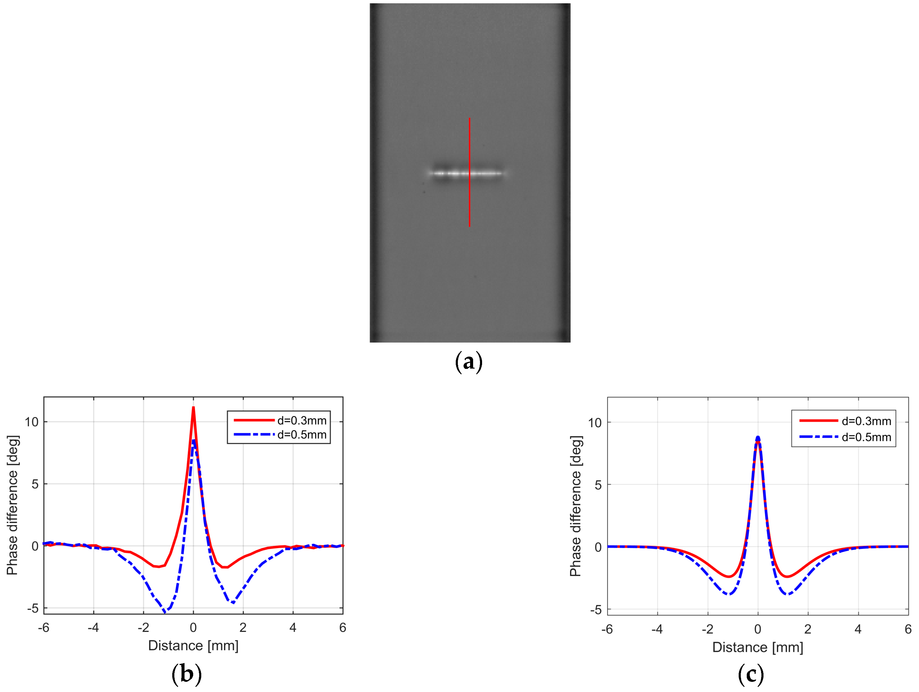
Figure 11.
(a) Microscopic cross section of a rolling lap defect; (b) simulated Joule heating around a crack in a ferro-magnetic material, f = 200 kHz.
Figure 11.
(a) Microscopic cross section of a rolling lap defect; (b) simulated Joule heating around a crack in a ferro-magnetic material, f = 200 kHz.

Figure 12.
Temperature distribution after 0.1 s (a) and after 1 s (b) heating pulses, simulated for the same crack as in Figure 11b. In the figures, dth/2 is also marked, which is approximately the distance where the phase is at its minimum.
Figure 12.
Temperature distribution after 0.1 s (a) and after 1 s (b) heating pulses, simulated for the same crack as in Figure 11b. In the figures, dth/2 is also marked, which is approximately the distance where the phase is at its minimum.

Figure 13.
(a) Phase around the crack shown in Figure 12 with different heating pulses; (b) phase for a vertical crack with the same d = 1 mm depth.
Figure 13.
(a) Phase around the crack shown in Figure 12 with different heating pulses; (b) phase for a vertical crack with the same d = 1 mm depth.
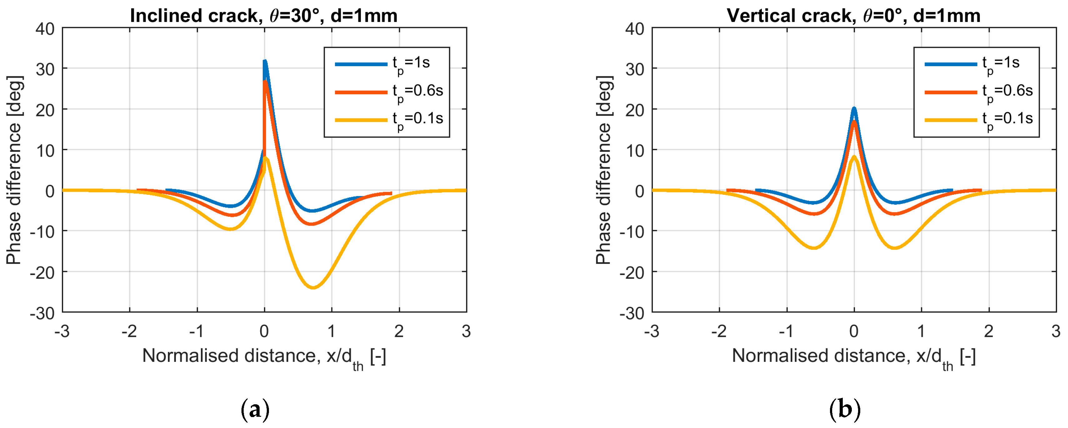
Figure 14.
Phase around cracks with the same depth d = 1 mm, but with different inclination angles simulated with the simu.2 model for ferro-magnetic steel properties. (a) Calculated for a 0.1 s pulse length and (b) for a 0.6 s heat duration.
Figure 14.
Phase around cracks with the same depth d = 1 mm, but with different inclination angles simulated with the simu.2 model for ferro-magnetic steel properties. (a) Calculated for a 0.1 s pulse length and (b) for a 0.6 s heat duration.

Figure 15.
Phase difference (a) and phase contrasts (b) for an asymmetrical phase distribution depending on the inclination angle of the crack with a 1 mm depth. For the definition of the displayed values, see Figure 14a.
Figure 15.
Phase difference (a) and phase contrasts (b) for an asymmetrical phase distribution depending on the inclination angle of the crack with a 1 mm depth. For the definition of the displayed values, see Figure 14a.

Figure 16.
(a) CAD data for four artificially created cracks in a laser-sintered sample; (b) phase image after a 0.1 s heating pulse; (c) profile through the phase image at the red marked position.
Figure 16.
(a) CAD data for four artificially created cracks in a laser-sintered sample; (b) phase image after a 0.1 s heating pulse; (c) profile through the phase image at the red marked position.

Figure 17.
Results for a steel sample with five artificial defects, each of them with a 1 mm depth and inclination angles from left to right of 75°, 60°, 45°, 30°, and 0°, respectively. (a) tpulse = 0.1s; (b) tpulse = 0.6 s; (c) profiles for different heating pulses.
Figure 17.
Results for a steel sample with five artificial defects, each of them with a 1 mm depth and inclination angles from left to right of 75°, 60°, 45°, 30°, and 0°, respectively. (a) tpulse = 0.1s; (b) tpulse = 0.6 s; (c) profiles for different heating pulses.

Figure 18.
Simulation model (simu.2) results shown in close-up to a vertical surface crack with a depth of 1 mm. Material: non-magnetic steel, properties are listed in Table 1. The excitation frequency is 200 kHz. (a) Eddy current streamlines; (b) Joule-heating.
Figure 18.
Simulation model (simu.2) results shown in close-up to a vertical surface crack with a depth of 1 mm. Material: non-magnetic steel, properties are listed in Table 1. The excitation frequency is 200 kHz. (a) Eddy current streamlines; (b) Joule-heating.

Figure 19.
Joule heating at the surface for d = 0.5 and 1 mm crack depths and for two different penetration depths depending on the distance (a) and abscissa normalized to (b).
Figure 19.
Joule heating at the surface for d = 0.5 and 1 mm crack depths and for two different penetration depths depending on the distance (a) and abscissa normalized to (b).

Figure 20.
(a) Temperature distribution after 0.1 s and (b) 1 s heating pulses for the same scenario as shown in Figure 18.
Figure 20.
(a) Temperature distribution after 0.1 s and (b) 1 s heating pulses for the same scenario as shown in Figure 18.
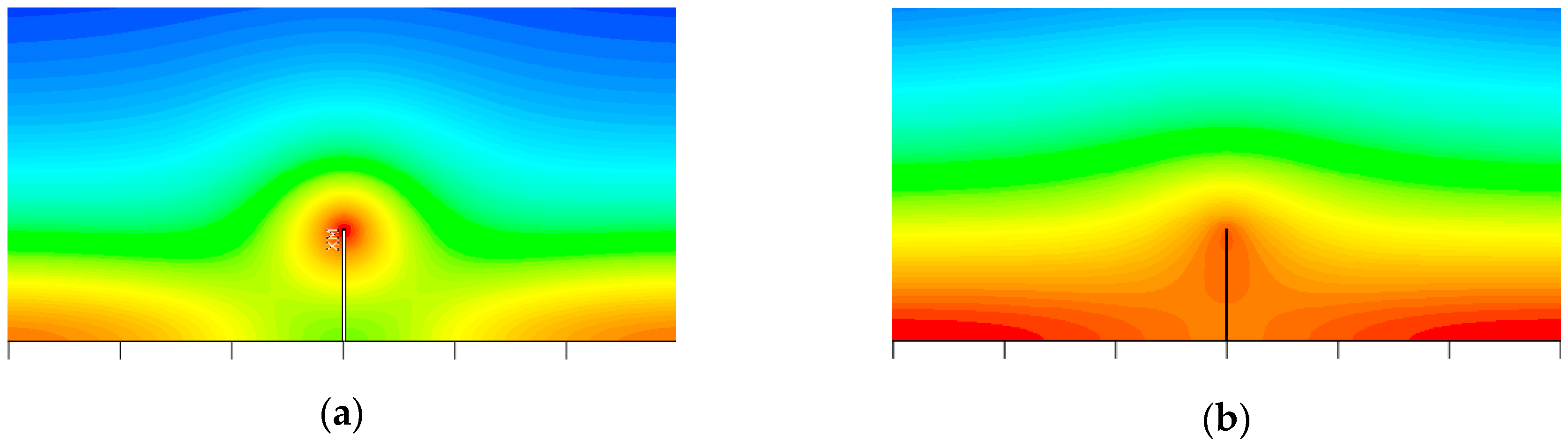
Figure 21.
Temperature at the crack position and at the sound surface distribution for 0.1 s (a) and 1 s (b) heating pulses for the same scenario shown in Figure 18 and Figure 20.

Figure 22.
(a) Phase distribution for different heating pulses for the same crack (d = 1 mm, δ = 1.35 mm); (b) phase for different crack depths after a 0.1 s heating pulse.
Figure 22.
(a) Phase distribution for different heating pulses for the same crack (d = 1 mm, δ = 1.35 mm); (b) phase for different crack depths after a 0.1 s heating pulse.

Figure 23.
Relative temperature contrast (a) and phase difference (b) for a crack with d = 1 mm calculated for different penetration depth values.
Figure 23.
Relative temperature contrast (a) and phase difference (b) for a crack with d = 1 mm calculated for different penetration depth values.

Figure 24.
(a) Phase difference for two cracks calculated for two different penetration depths; (b) phase difference in a normalized manner for ferro-magnetic (dash-dot lines) and for non-magnetic (solid lines) steel. Values marked with “+” are calculated for d = 1 mm and with “o” for d = 0.5 mm.
Figure 24.
(a) Phase difference for two cracks calculated for two different penetration depths; (b) phase difference in a normalized manner for ferro-magnetic (dash-dot lines) and for non-magnetic (solid lines) steel. Values marked with “+” are calculated for d = 1 mm and with “o” for d = 0.5 mm.
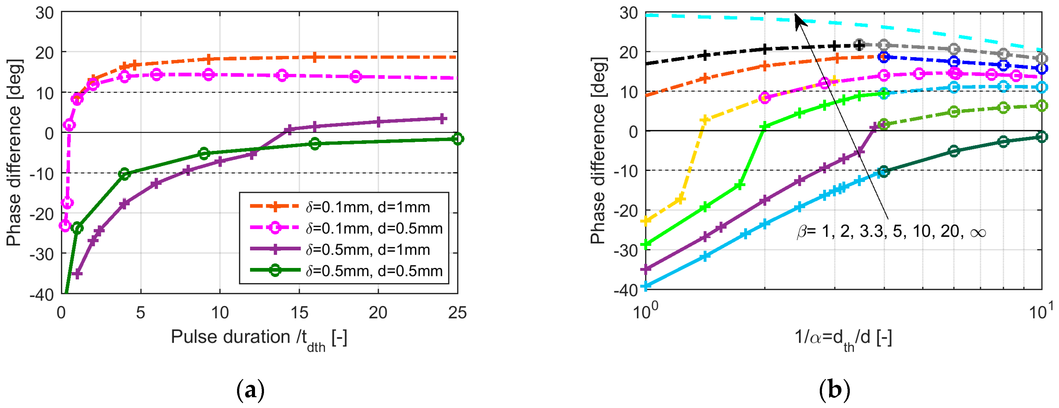
Figure 25.
(a) Phase difference depending on the crack depths, calculated for two penetration depths and for three heating pulse durations; (b) normalized curves for ferro-magnetic (dash-dot lines) and for non-magnetic (solid lines) steel. Values marked with “+” are calculated for d = 1 mm and with “o” for d = 0.5 mm; both figures also show the same analytically calculated curves plotted as per Figure 6b,d.
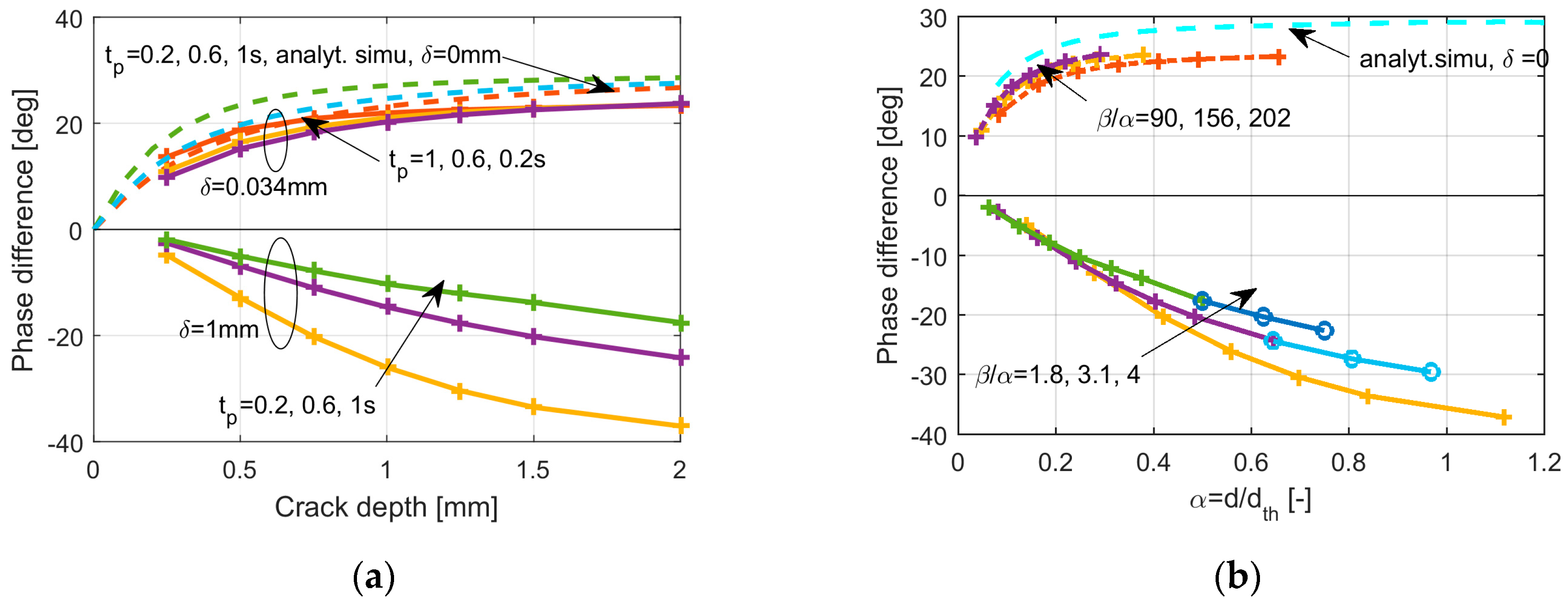
Figure 26.
Phase images for a non-magnetic steel sample with five artificial defects, with 2, 1.5, 1, 0.75, and 0.5 mm depths, from left to right, respectively. (a) tpulse = 0.2 s; (b) tpulse = 0.6 s; (c) profiles through the phase images for different heating pulses.
Figure 26.
Phase images for a non-magnetic steel sample with five artificial defects, with 2, 1.5, 1, 0.75, and 0.5 mm depths, from left to right, respectively. (a) tpulse = 0.2 s; (b) tpulse = 0.6 s; (c) profiles through the phase images for different heating pulses.

Figure 27.
Results for a titanium wire with a rolling lap. (a) temperature curves; (b) phase image with a 0.1 s heating pulse; (c) phase profiles with different pulse lengths.
Figure 27.
Results for a titanium wire with a rolling lap. (a) temperature curves; (b) phase image with a 0.1 s heating pulse; (c) phase profiles with different pulse lengths.

Figure 28.
Simulation model (simu.2) results shown in close-up to an inclined surface crack θ = 30° and with a depth of 1 mm. Material: non-magnetic steel, the properties are listed in Table 1. Excitation frequency is 200 kHz. (a) Eddy current streamlines; (b) Joule-heating.
Figure 28.
Simulation model (simu.2) results shown in close-up to an inclined surface crack θ = 30° and with a depth of 1 mm. Material: non-magnetic steel, the properties are listed in Table 1. Excitation frequency is 200 kHz. (a) Eddy current streamlines; (b) Joule-heating.

Figure 29.
Temperature distribution after 0.1 s (a) and 1 s. (b) Heating pulse for the same scenario as in Figure 28.
Figure 29.
Temperature distribution after 0.1 s (a) and 1 s. (b) Heating pulse for the same scenario as in Figure 28.

Figure 30.
(a) Phase around the crack as shown in Figure 28 and Figure 29 for different heating pulses; (b) phase for a vertical crack with the same d = 1 mm depth.

Figure 31.
Phase around cracks with the same depth d = 1 mm, but with different inclination angles simulated with the simu.2 model for steel properties; (a) calculated for a 0.1 s pulse length and (b) for a 0.6 s heating duration.
Figure 31.
Phase around cracks with the same depth d = 1 mm, but with different inclination angles simulated with the simu.2 model for steel properties; (a) calculated for a 0.1 s pulse length and (b) for a 0.6 s heating duration.

Figure 32.
Phase difference (a) and phase contrasts (b) for an asymmetrical phase distribution depending on the inclination angle of the crack with a 1 mm depth. For the definition of the displayed values see Figure 31a.
Figure 32.
Phase difference (a) and phase contrasts (b) for an asymmetrical phase distribution depending on the inclination angle of the crack with a 1 mm depth. For the definition of the displayed values see Figure 31a.

Figure 33.
Phase images for a non-magnetic steel sample with five artificial defects, each of them with a 1 mm depth, and inclination angles of 75°, 60°, 45°, 30° and 0° from left to right, respectively; (a) tpulse = 0.1 s; (b) tpulse = 0.6 s; (c) profiles for different heating pulses.
Figure 33.
Phase images for a non-magnetic steel sample with five artificial defects, each of them with a 1 mm depth, and inclination angles of 75°, 60°, 45°, 30° and 0° from left to right, respectively; (a) tpulse = 0.1 s; (b) tpulse = 0.6 s; (c) profiles for different heating pulses.


Table 1.
Material parameters.
| Material | Electrical Conductivity σ (Ω −1 m−1) | Relative Permeability µr (-) | Thermal Conductivity λ (W m−1 K−1) | Thermal Diffusivity κ (m2 s−1) | Penetration Depth δ, If f = 200 kHz (mm) | Th. Diffusion Length dth, If t = 0.1 s (mm) |
|---|---|---|---|---|---|---|
| Steel ferro-magn. | 1.85 × 10⁶ | 600 | 40 | 1.16 × 10⁻⁵ | 0.034 | 2.16 |
| Steel AISI304 non-magn. | 7 × 10⁵ | 1 | 16 | 4 × 10⁻⁶ | 1.35 | 1.26 |
Table 2.
The models and four cases for which the models can be applied (d: crack depth; δ: eddy current penetration depth).
Table 2.
The models and four cases for which the models can be applied (d: crack depth; δ: eddy current penetration depth).
| Crack Types | Cases | Analytical Model | FEM simu.1 (Surface Heat Flux) | FEM simu.2 (Inductive Heating) |
|---|---|---|---|---|
| Vertical crack | Case 1 δ ~0, δ << d | δ = 0 | δ = 0 | δ << d |
| Case 2 δ ~d | - | - | δ ~d | |
| Inclined crack | Case 3 δ ~0, δ << d | - | δ = 0 | δ << d |
| Case 4 δ ~d | - | - | δ ~d |
© 2018 by the author. Licensee MDPI, Basel, Switzerland. This article is an open access article distributed under the terms and conditions of the Creative Commons Attribution (CC BY) license (http://creativecommons.org/licenses/by/4.0/).
Share and Cite
MDPI and ACS Style
Oswald-Tranta, B. Induction Thermography for Surface Crack Detection and Depth Determination. Appl. Sci. 2018, 8, 257. https://doi.org/10.3390/app8020257
AMA Style
Oswald-Tranta B. Induction Thermography for Surface Crack Detection and Depth Determination. Applied Sciences. 2018; 8(2):257. https://doi.org/10.3390/app8020257
Chicago/Turabian StyleOswald-Tranta, Beate. 2018. "Induction Thermography for Surface Crack Detection and Depth Determination" Applied Sciences 8, no. 2: 257. https://doi.org/10.3390/app8020257
Note that from the first issue of 2016, this journal uses article numbers instead of page numbers. See further details here.