Study on SPH Viscosity Term Formulations

1
College of Shipbuilding Engineering, Harbin Engineering University, Harbin 150001, China
2
School of Mathematics, Computer Science and Engineering, City University of London, London EC1V 0HB, UK
3
State Key Laboratory of Hydraulics and Mountain River Engineering, Sichuan University, Chengdu 610065, China
*
Author to whom correspondence should be addressed.
Appl. Sci. 2018, 8(2), 249; https://doi.org/10.3390/app8020249
Submission received: 25 December 2017
/
Revised: 20 January 2018
/
Accepted: 1 February 2018
/
Published: 7 February 2018
Abstract
:Featured Application
The proposed study contributes to the mesh-free numerical modeling field through the examinations of several viscosity term formulations. By simulating benchmark viscosity-dominated flows in engineering practice, the optimal viscosity scheme has been found to work with the Smoothed Particle Hydrodynamics (SPH) method.
Abstract
For viscosity-dominated flows, the viscous effect plays a much more important role. Since the viscosity term in SPH-governing (Smoothed Particle Hydrodynamics) equations involves the discretization of a second-order derivative, its treatment could be much more challenging than that of a first-order derivative, such as the pressure gradient. The present paper summarizes a series of improved methods for modeling the second-order viscosity force term. By using a benchmark patch test, the numerical accuracy and efficiency of different approaches are evaluated under both uniform and non-uniform particle configurations. Then these viscosity force models are used to compute a documented lid-driven cavity flow and its interaction with a cylinder, from which the most recommended viscosity term formulation has been identified.
1. Introduction
Free surface flow simulations have always generated substantial theoretical and practical interests. Bontozoglou [1] used the spectral spatial discretization method for the laminar film flow along a periodic wall. Scholle et al. [2] used the Finite Element Method (FEM) and complex variable method for modeling the film over corrugated surfaces. Marner et al. [3] developed a potential-velocity formulation of the Navier-Stokes (N-S) equations by using the least square FEM approach. More recently, Marner et al. [4] proposed a generalized complex-valued first integral of the N-S equations for the unsteady Couette flows in a corrugated channel system. Compared with these, the Smoothed Particle Hydrodynamics (SPH) method is equipped with the unique advantage of tracking the free surfaces with much larger deformation even leading to violent breaking.
Since the concept of the mesh-free SPH method was introduced to model hydrodynamic flows [5], SPH has shown its promising performance in a wide range of free surface flows. The benchmark model applications have been documented in the study of dam-break flow [6], wave-structure interaction [7], inflow and outflow [8], porous flow [9] and multi-phase flow [10]. Besides, the shallow water equations (SWEs) were also solved by SPH for the flows in a large area where the vertical flow variations can be reasonably ignored [11,12]. More complex SPH model applications involving the movable bed, sediment and pollutant transport were reported by [13] and Pahar and Dhar [14,15]. Besides, some recent weakly compressible SPH (WCSPH) works include a robust procedure to filter the high-frequency oscillations in the pressure field arising from the use of the artificial sound speed, in the field of both strong dynamics [16] and slow dynamics [17]. These were based on the improvement of certain diffusive approaches (e.g., [18]) in which the numerical noise was just alleviated through the additional post-processing of the pressure data.
The above-mentioned free surface flows are dominated by the gravity and pressure influence. To improve the modeling accuracy of such flows, quite a few studies have been done to enhance the SPH pressure formulation [19] and the pressure solution in either the WCSPH [20] or incompressible SPH (ISPH) [21]. On the other hand, there is another kind of the flow, which is also of great engineering interest, but dominated by the influence of the flow viscosity, such as a lid-driven cavity flow. To realistically simulate these, the treatment of the viscosity force term in the N-S equations becomes important. As compared with the established studies on the pressure formulation, the research on the viscosity term was paid much less attention in the SPH field, probably due to its minor role in the medium-to-high Reynolds number flows commonly found in the free surface applications. Besides, one technical difficulty arises from the fact that the viscosity term involves a second-order derivative calculation, while the pressure term is only of the first-order, and therefore the numerical treatment becomes more complex.
The earliest viscosity term treatment in SPH adopted the artificial viscosity approach proposed by Monaghan [5] to avoid the particle instability and thus to maintain the computational stability. The effect of relevant parameters in the artificial formulation was extensively explored by De Padova et al. [22] in their SPH simulation of six different regular waves. Following the establishment of the projection SPH [23] and ISPH [24], the real viscosity term form based on Morris et al. [25] has been more widely used. Compared with the artificial viscosity, the real viscosity has a clearer physical implication and it also performs much better in the practical SPH applications. To improve viscosity performance in reproducing the broken free surfaces, Khayyer et al. [26] made one step-forward correction by comprehensively addressing the linear and angular momentum conservations. In a turbulent flow where the particle resolution is insufficient, an eddy viscosity term has been proposed by Gotoh et al. [27] using the sub-particle-scale (SPS) shear stress model. Recently, quite a few viscosity corrections were reported to show their importance in viscosity-dominated flow applications. For example, Basa et al. [28] reviewed the early viscosity formulations for a wide range of Reynolds numbers using a Poiseuille channel and lid-driven cavity flow. Colagrossi et al. [29] used three viscosity models to investigate the consistency and energy mechanisms of the SPH scheme. Grenier et al. [30] adopted the renormalized Morris et al. formulation with an inter-particle dynamic viscosity coefficient to model the merging process of two viscous bubbles. The latest work in the field could be attributed to Liu and Liu [31], who studied the viscous forces in a Poiseuille flow on both the regular and irregular particle configurations.
Quite a few established approaches treat the real viscosity term by using a hybrid formulation of the SPH first-order derivative combined with a finite difference representation. However, the viscosity term appears in the N-S equations as a second-order derivative. A more refined treatment of this should greatly improve the SPH performance in viscosity-dominated flows. In a recent review work, Ma et al. [32] comprehensively summarized all existing formulations of the Laplacian term used in the pressure Poisson equation (PPE) of ISPH models. Laplacian is a second-order derivative representation, which is basically similar to the viscosity term. Thus, the present study aims to model the viscosity term by following similar treatment algorithms used in the Laplacian formulation and then further examine the new model performance.
The paper is structured as follows. The next chapter briefly reviews the ISPH methodology. Then a review on several second-order derivative approximations used in the PPE is made and the associated discretization schemes are transformed to model the viscosity term. After this a detailed benchmark patch test based on a polynomial function is carried out to evaluate the accuracy and efficiency of different viscosity force models, under both the regular and irregular particle configurations. Finally, two viscosity-dominated flows are used to further demonstrate the importance of the viscosity term effect in practical model applications, including the lid-driven cavity flow and its interaction with an inside cylinder.
2. Materials and Methods I—General ISPH Methodology
The basic concept of SPH is that a particle is fundamental in the Lagrangian description and the motion of a continuum can be represented with high accuracy by simulating the motion of a large number of such particles. Through the use of the integral interpolants, any field variables can be expressed by the integrals that are approximated by the summation interpolants over the neighboring particles. Similarly, the spatial derivatives at each particle location can also be evaluated by the summation interpolants. The derivatives are computed based on the kernel function, which can be obtained analytically. For example, the particle approximation of a value and its gradient can be shown as
where is the reference particle and represents all the neighboring particles; is the number of particles for the summation; is the particle mass; is the particle density; and are the positions of the particle; is the SPH interpolation kernel function; represents the gradient of the kernel taken with respect to the reference particle; and is the kernel smoothing length. The kernel function can have many different forms and a cubic spline kernel is used in this paper due to its computational accuracy and efficiency. In a practical SPH computation, the gradient of the pressure and divergence of the velocity are usually calculated by
where is defined as the velocity difference.
In an ISPH approach the fluid density is assumed to be constant. Therefore, the mass and momentum conservation equations, i.e., N-S equations, can be written in the following quasi-Lagrangian description as
where is the time; is the gravitational acceleration; and is the kinematic viscosity.
The two-step projection method [24] is used to solve the velocity and pressure in Equations (5) and (6). The first step is the prediction of velocity in the time domain without including the pressure term. The intermediate particle velocity and position are obtained as
where and are the velocity and position of particle at time ; is the time step; is the velocity change; and and are the intermediate velocity and position of particle.
In the second step the pressure term is used, leading to a correction of the particle velocity as
Then the new time-step values are updated by
where and are the velocity and position of the particle at new time step.
According to Zheng et al. [33], the following form of the pressure Poisson equation, which includes the divergence of flow velocity and the variance of particle density as the mixed source term, is used to solve the fluid pressure for enhancing the model performance. This equation was derived from the combination of the continuity equation (Equation (5)) and the velocity correction (Equation (10)), based on the compressible form of the continuity equation .
where is a weighting coefficient and a value of 0.01 is used from the computational experiences.
The left-hand-side of Equation (13), i.e., the Laplacian term, is commonly discretized by merging the standard SPH gradient formulation with a first-order finite difference scheme as
where is defined as the pressure difference and the position difference; and is a small number to avoid singularity.
In the present ISPH model, the kinematic free surface boundary conditions can be automatically satisfied due to the mesh-free nature of the model. The free surface particles are identified by using the auxiliary functions combined with the particle number density criterion by following Zheng et al. [33]. Besides, to improve the treatment of the solid boundary conditions, a high accuracy of the Simplified Finite Difference Interpolation (SFDI) scheme is used on the solid walls to solve the PPE. One promising feature of this pressure solution scheme is that the normal pressure gradient is computed on the solid boundary without the use of the mirror particles. This can improve the simulation accuracy near the solid wall, and meanwhile reduce the CPU cost.
In a viscous flow, the dynamic boundary condition should be an exact equilibrium between the pressure, viscous stress and surface tension, as pointed out by Scholle et al. [2]. Since there is no free surface involved in the present model applications, a simple approximation based on the zero pressure only is imposed as the dynamic free surface boundary condition.
3. Materials and Methods II—SPH Viscosity Term Formulations
Ma et al. [32] comprehensively reviewed the established SPH discretization schemes for the second-order Laplacian term in the PPE. In this section, four representative formulations are selected to model the viscosity term as below.
3.1. Hybrid Form Viscosity Force Model-01 (VISC-01)
This was proposed by Cummins and Rudman [23] by using a hybrid of the standard SPH gradient formulation combined with a first-order finite difference scheme. It can also be obtained through the analysis of the viscous stress such as documented by Morris et al. [25]. Shao and Lo [24] adopted this form in their ISPH model. This kind of the viscosity term representation is usually written as
where indicates the spatial component.
3.2. Direct Form Viscosity Force Model-02 (VISC-02)
Originally aiming to improve the accuracy of Laplacian approximation, Gotoh et al. [34] derived a new form of the equations by directly taking the divergence of a SPH gradient model. This was actually founded on the twice differentiation of the SPH interpolant, and therefore it intrinsically contains the second-derivative of a kernel. By adopting a similar approach of the derivation, the viscosity term can be modeled as
However, as pointed out by Gotoh et al. [34], this formulation is very sensitive to the particle disorder, especially when the order of the kernel function is low.
3.3. Schwaiger Form Viscosity Force Model-03 (VISC-03)
Schwaiger [35] proposed a higher-order derivation approach, which is based on the gradient approximations used in the thermal, viscous and pressure projection problems, but including the higher-order terms in appropriate Taylor series. By substituting the pressure variable in the original formulation of Schwaiger [35] with the flow velocity, the following viscosity representation can be obtained
where is the number of dimensions; and is defined. The size of and is 2 × 2 in a 2D and 3 × 3 in a 3D application. Schwaiger’s approach requires the inverse operations of the matrices and at each fluid particle, so it could cost a little more in computational expenses. The original formulation was developed for the thermal diffusion solutions, and Jian et al. [36] used this for the fluid-structure interactions in their ISPH approach.
3.4. Oger, Hosseini and Feng, Khayyer Form Viscosity Force Model-04 (VISC-04)
Oger et al. [37] studied a wide range of the correction procedures to improve the accuracy of kernel approximations and they proposed a renormalization technique from the discrete version of the Eulerian equations. Based on the study, they eventually constructed a correction matrix to account for the irregular distribution of the neighboring particles around the reference one. This is written in the form of the viscosity term representation as
where the correction matrix has the same form as Equation (19) for a 2D problem, while it becomes a 3 × 3 matrix in 3D. It should be noted that in a follow-on study, Hosseini and Feng [38] refined this approximation to ensure the gradient function being accurately calculated. Also Khayyer et al. [26] developed a similar correction technique on the kernel gradient to calculate the viscous forces, therefore both the linear and the angular momentums are exactly conserved in their ISPH model.
4. Results I—Analysis of Model Accuracy through Benchmark Tests
In this section, the detailed numerical investigations are made into the convergence and accuracy behaviors of the above four viscosity force models, under both the uniform and random particle distributions in a 2D framework. The error of the numerical result is quantified as
where is the mean numerical error; is the numerical value; is the analytical solution; and is the number of sampling points in the whole domain.
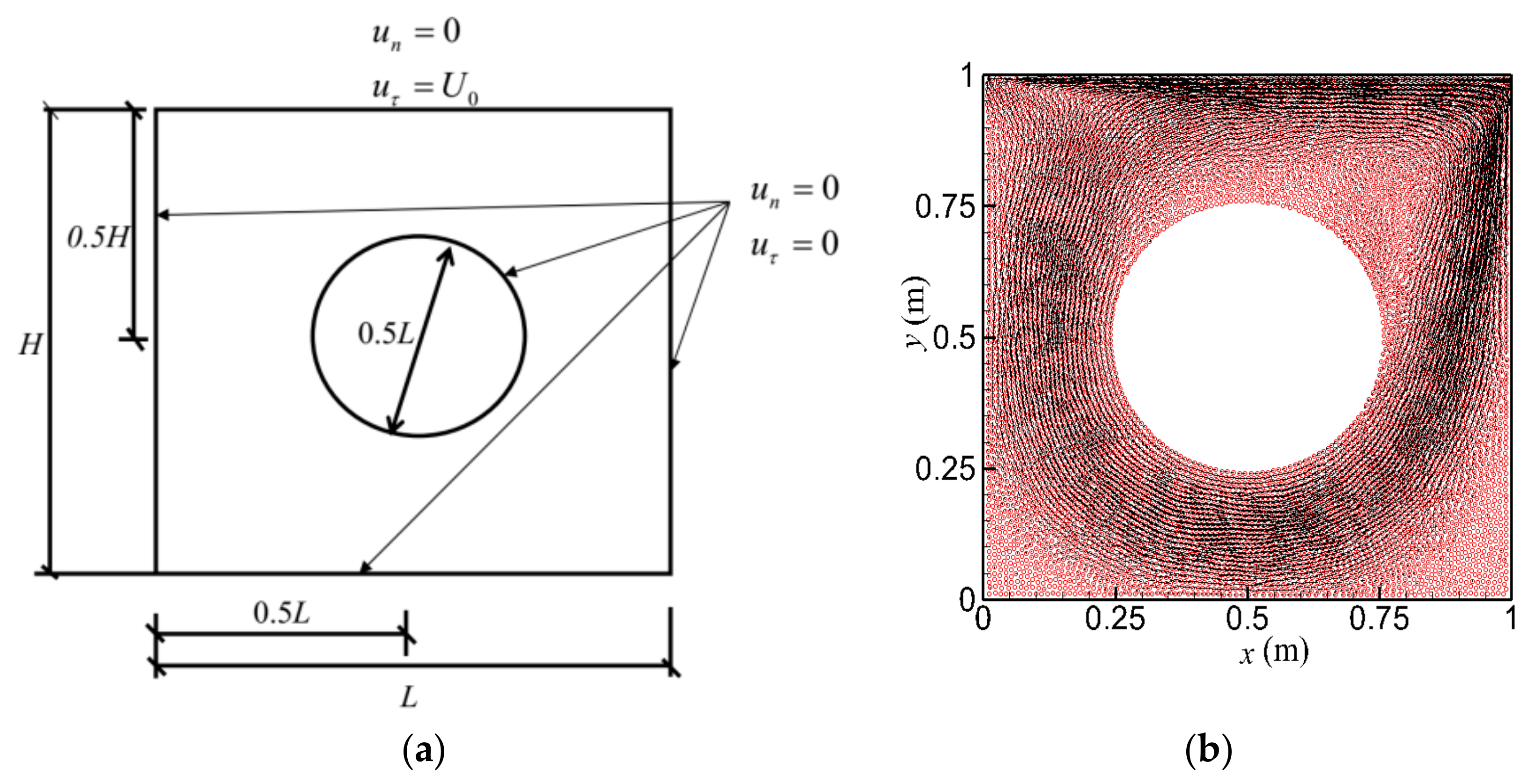
The computational domain of the test is chosen as a square with the side length of 1 m as shown in Figure 1. The test function uses a polynomial of second-order expressed by . The SPH kernel function used is a cubic spline kernel [5] normalized in 2D. The SPH particles are arranged in a uniform and non-uniform configuration, respectively. In the former case a uniform Cartesian configuration of the particles is used, while in the latter case the particle positions are determined by , where is a random number with a value (0, 1) through the quasi-random number generator, and is the particle size vector in 2D under the uniform distribution condition. A sample particle distribution is also illustrated in Figure 1 for the particle number of 400. In the following test, five different particle resolutions are considered, including a total number of 20 × 20, 40 × 40, 60 × 60, 80 × 80, 100 × 100 particles. This corresponds to the particle size of = 0.05 m, 0.025 m, 0.01667 m, 0.0125 m and 0.01 m, respectively.
4.1. Accuracy under Uniform Distribution of the Particles
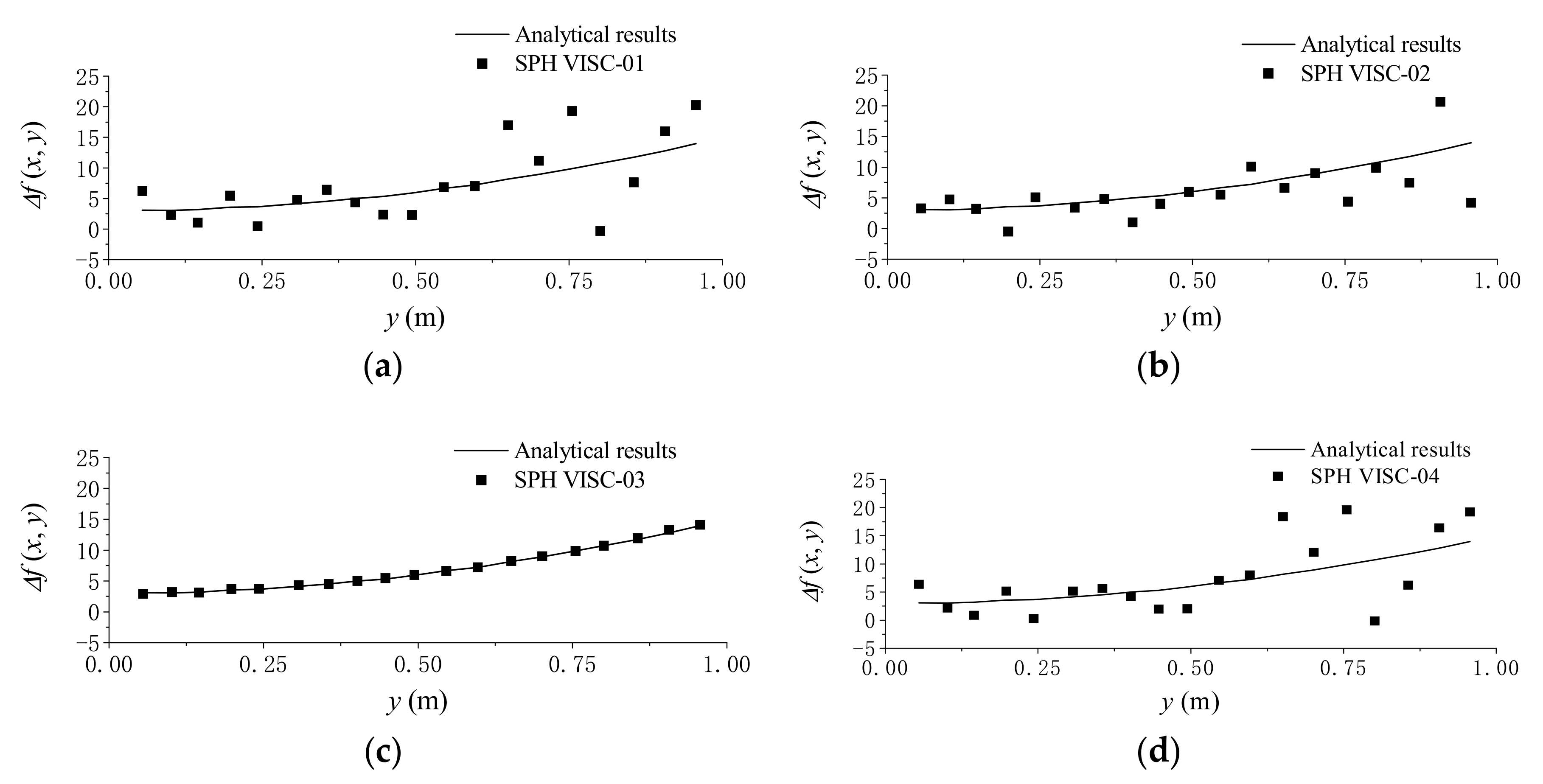
To examine the second-order derivative of the polynomial function, i.e., , Figure 2 gives the comparisons between the analytical and numerical results computed by the different SPH viscosity force models, at = 0.5 m and = (0, 1) m, under uniform particle distribution with a particle size = 0.05 m. As shown in Figure 2, all the four viscosity methods led to a very good agreement with the analytical results when the particles are uniformly distributed.
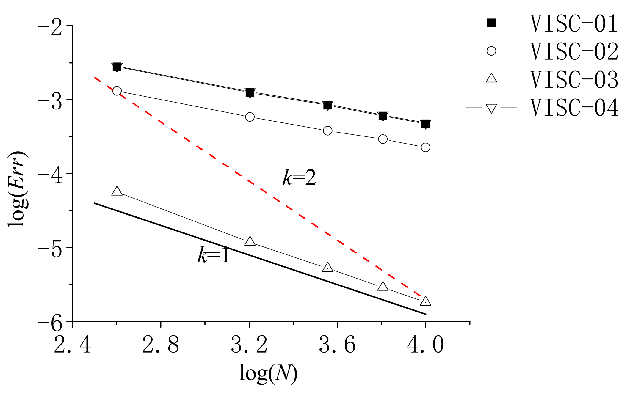
As a sensitivity test, Table 1 gives the mean errors defined by Equation (21) for the different particle numbers computed by the four different viscosity force models. Figure 3 further gives the convergence rate in the form of the total particle number and the numerical error , in which k refers to the convergence ratio. That is to say, k = 1 indicates the numerical model can achieve the first-order convergence, while k = 2 the second-order convergence. Both Table 1 and Figure 3 are provided based on the uniform particle distributions. According to Table 1, the accuracy of VISC-01 is the lowest, while VISC-03 and VISC-04 can achieve the highest accuracy, and VISC-02 lies somewhere in the between. This conclusion is further consolidated by Figure 3, which clearly shows the convergence rate of each viscosity force model. It is well indicated that VISC-01 and VISC-02 are around the first-order accuracy, while VISC-03 and VISC-04 can obtain the second-order.
4.2. Accuracy under Non-Uniform Distribution of the Particles
For the non-uniform particle distributions, Figure 4 gives the comparisons of the analytical and numerical results computed by using four different viscosity force models. In this case, is around (0.5 − 0.1 , 0.5 + 0.1 ) m and still ranges within (0, 1) m. The particles are irregularly distributed within the domain and the initial particle size is = 0.05 m. According to the results shown in Figure 4, VISC-03 can achieve the most accurate result, while the errors of VISC-01 and VISC-04 are the highest. This situation is completely different from the uniform particle distribution, as shown in Figure 2.
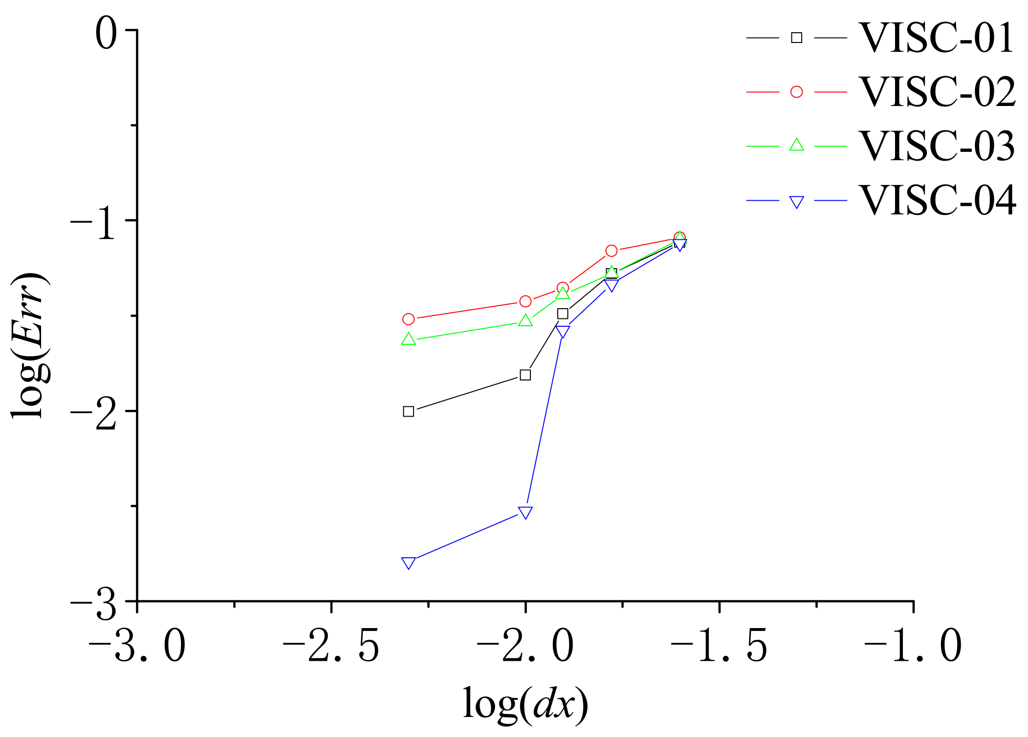
Furthermore, Table 2 gives the mean errors for the different particle numbers computed by the different viscosity methods, and Figure 5 gives the convergence rate corresponding to the particle number and error , under the non-uniform particle configurations. From Table 2, the results of VISC-03 show the best accuracy, while VISC-01 and VISC-04 results demonstrate the least satisfactory performance. In comparison, VISC-02 results are in the middle range. Also, it can be found that the errors of VISC-04 change a lot with the different particle numbers. Besides, Figure 5 quantitatively shows that the convergence rate of VISC-03 is near the first-order accuracy, while the other three models cannot reach this level of the convergence. Similar results are also observed on VISC-01 and VISC-04.
4.3. Analysis of CPU Expenses
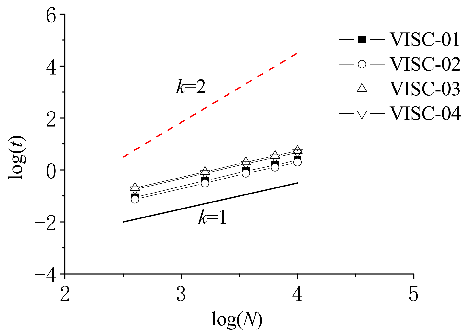
To show the CPU efficiency of different viscosity methods, Table 3 gives the comparisons of CPU time corresponding to the different particle numbers and viscosity force models, when the particles are under the irregular distribution. For the present benchmark patch test, the CPU time under the regular distribution of the particles is nearly the same as that under the irregular distribution. It shows that the CPU cost of VISC-02 is the cheapest, while that of VISC-03 is the heaviest. In contrast, the CPU time of VISC-01 is a little longer than that of VISC-02, but it is much shorter than that of VISC-04. Figure 6 provides the convergence analysis of each viscosity force model in view of the CPU time, in which a unanimously first-order convergence rate is found among the four models.
4.4. Brief Evaluations of Four Viscosity Force Models
Based on the above accuracy and efficiency analysis, it shows that VISC-03 can attain the highest accuracy under either the uniform or non-uniform particle distributions. In comparison, VISC-04 can achieve the similar accuracy but only under the uniform particle distributions, while its accuracy degrades to that of VISC-01 when the particles are randomly distributed. Among these the accuracy of VISC-02 lies in somewhere in-between. However, in view of the CPU efficiency, VISC-02 is the fastest model but VISC-03 is the slowest. To further examine different viscosity force models in a practical ISPH simulation, more benchmark test cases will be studied in the next section.
Besides, it has also been found that the mean errors obtained by VISC-03 and VISC-04 are always the same in case of the uniform particle distribution while significant differences occur for the non-uniform distribution. This is due to the fact that, under the uniform distribution of the particles, the second term on the right-hand-side of Equation (17) becomes zero, and also becomes unity. Therefore, Equations (17) and (20) become exactly identical, leading to the same performance of VISC-03 and VISC-04. On the other hand, these conditions do not hold under the non-uniform particle distribution, and the numerical differences become significantly larger as a result.
5. Results II—Model Application in Practical Viscous Flows
In order to demonstrate the effect of four methods of viscosity term calculation, this section presents two numerical tests on the viscous flow modeling, which are based on the benchmarks of the lid-driven flow and its interaction with an inside cylinder. This would provide more useful information on the different viscosity force models in practical situation. The lid-driven flows have been widely used as a benchmark validation case for the different SPH viscosity force models. For example, Zheng et al. [33] used an artificial viscosity, Leroy et al. [39] used a turbulent dynamic viscosity, Aly et al. [40] used a Morris formula, and Yildiz et al. [41] derived a more general second-order derivative approximation based on the Taylor series expansion and the concept of second- and fourth-order isotropic tensors.
5.1. Lid-Driven Flow
A lid-driven flow within a 2D square cavity of height H and width L is considered in the present section. The two side walls and the bottom wall of the cavity are stationary, while the top wall experiences a constant forced motion. The velocity of the top wall in the x-direction is given by . In the numerical study, the following parameters are used: H = L = 1.0 m, kinematic viscosity = 0.001 m2/s, and , where = 1.0 m/s is adopted.
Figure 7 gives the vector plots of lid-driven flow forced by the uniform motion of the top lid for the Reynolds number Re = 1000, with two different particle numbers of N = 1600 and 10,000, respectively. The computational time step = 0.001 s is used. The simulation was carried out until t = 40 s when the velocity distribution reached the stable state. To validate the numerical results, Figure 8 gives the comparisons on the velocity amplitude distribution computed by the OpenFOAM (i.e., Open source Field Operation and Manipulation, [42]) and ISPH (VISC-04), in which a similar velocity field has been found from the two model results.
OpenFOAM is a C++ toolbox for the development of customized numerical solvers, and pre-/post-processing utilities for the solution of continuum mechanics including CFD problems. OpenFOAM uses the finite volume method (FVM) and is a typically mesh-based numerical model. The FVM uses a co-located methodology on an unstructured grid with arbitrary grid element. A variety of available interpolation, discretization and matrix solution schemes can be selected at runtime and both the implicit and explicit solution techniques are accessible to the end-users.
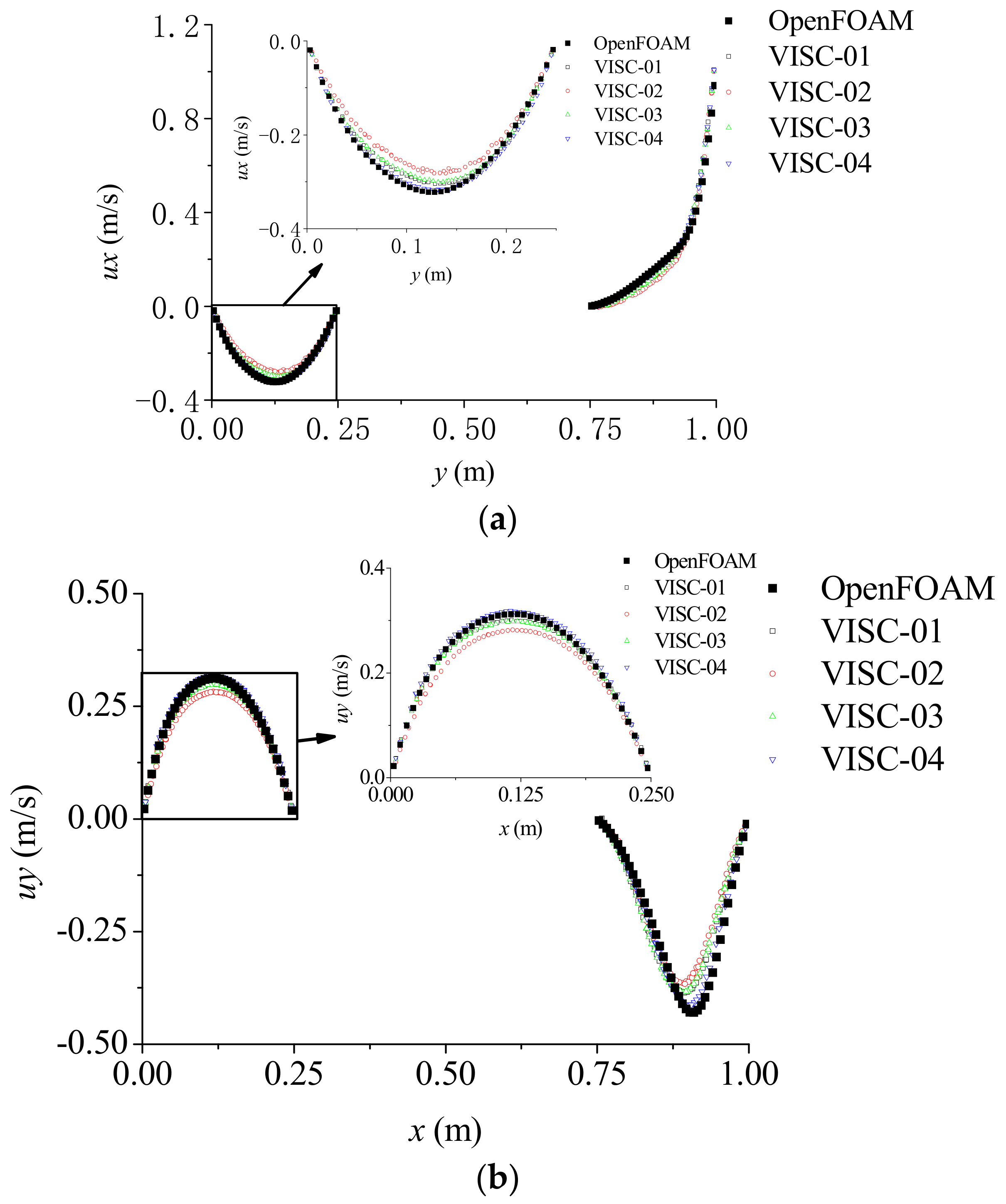
In order to quantify the accuracy of different viscosity calculation methods, Figure 9 gives the comparisons of velocity component distributions ux at x = 0.5 m and uy at y = 0.5 m with the experimental data of Ghia et al. [43] and OpenFOAM. In this case, the following computational parameters are used: particle size dx = 0.005 m, simulation time t = 40 s and Reynolds number Re = 1000. It is shown from Figure 9 that the results obtained by the four viscosity calculation methods are generally quite similar to each other. By examining the enlarged chart where the velocity experiences a larger gradient, however, it can be found that the results obtained by VISC-04 can get the best agreement with the experimental data.
Furthermore, for the purpose of model convergence analysis, Figure 10 gives the errors in minimum ux value between the experimental data and various ISPH results for the different particle resolutions. The computational results of OpenFOAM are also shown for a comparison. The numerical error is defined by =, where is the numerical minimum and is the experimental one. According to the results in Figure 10, all errors obtained by the ISPH viscosity force models unanimously show a decreasing trend with a decrease in the particle size, i.e., an increase in the particle number. Meanwhile, VISC-04 can achieve the smallest errors among all viscosity force models under the same particle scale.
5.2. Lid-Driven Flow with an Inside Cylinder
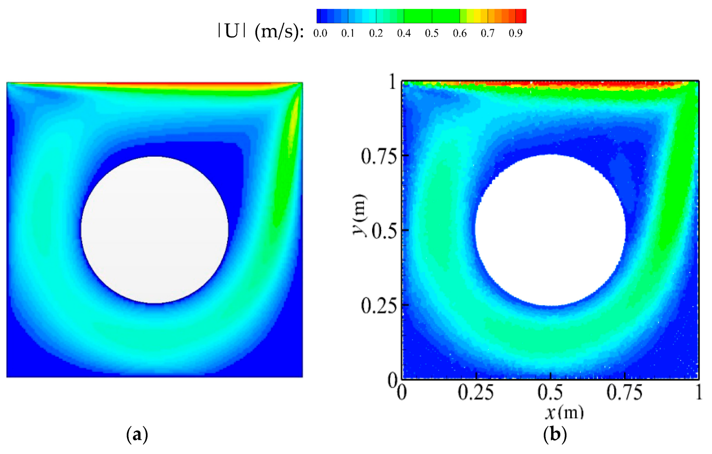
To provide a further robust evaluation on the proposed ISPH viscosity force models, this section explores a more complex lid-driven flow case with a cylinder inside. The schematic set up of the model is shown in Figure 11a. There is a cylinder inside the cavity region, with its diameter being d = 0.5 L. The 2D square cavity has a height H and width L, with the dimensions of H = L = 1.0 m. The center of the cylinder is located at (0.5 L, 0.5 H). The wall boundary of both the cylinder and the cavity region is set as the non-slip and non-penetration condition in the tangential and normal directions, respectively, where ur and un indicate the velocity component in each direction. The velocity of the top wall of the cavity in the x-direction is given by U0 = 1.0 m/s, which leads to a Reynolds number Re = 1000. The other computational parameters are kept unchanged as those used in Section 5.1. Based on the ISPH model simulations (with VISC-04), Figure 11b gives the result of velocity vector plots of the cavity flow at particle number N = 10,000 and simulation time t = 40 s, when the steady results are achieved. Figure 12 shows the comparison of velocity amplitude patterns between the ISPH and OpenFOAM computations, and a qualitatively good agreement has been found.
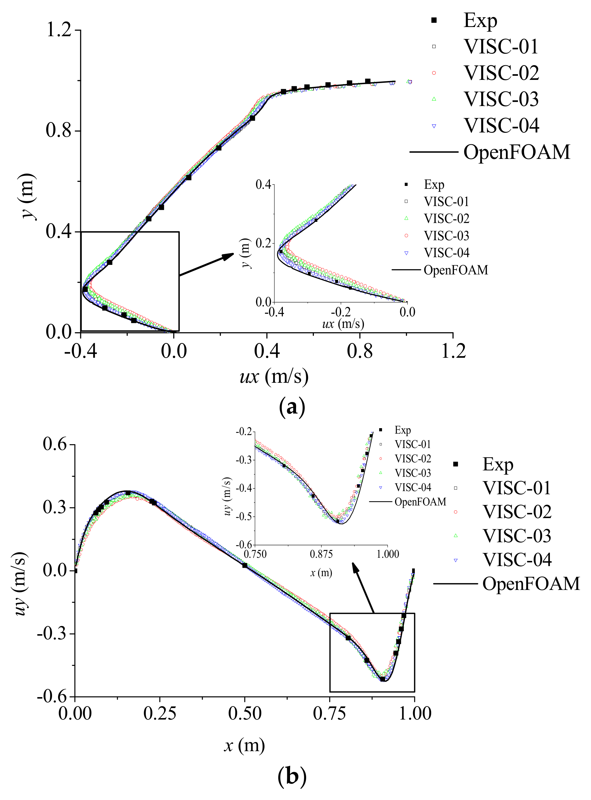
To finally examine the performance of different viscosity force models, Figure 13 gives the comparisons of velocity ux distributions at x = 0.5 m and uy distributions at y = 0.5 m, computed by the ISPHs and FVM-based OpenFOAM. In this case, the computational parameters are: particle size dx = 0.005 m, time t = 40 s and Reynolds number Re = 1000. As shown in Figure 13, the results obtained by the four viscosity calculation methods are quite similar to each other, except the enlarged portion (where the velocity profiles change sharply) shows that the result obtained by VISC-04 is the most satisfactory compared with the OpenFOAM results. It is also noticeable that OpenFOAM generally gives higher values of the velocity than ISPH for both the lid-driven flow and the lid-driven flow with an inside cylinder.
For convergence and error analysis, Figure 14 gives the numerical errors of minimum velocity ux of various ISPH viscosity force models under different particle resolutions, where Err is defined as the same error used in the previous section. Again all the ISPH errors decrease with the deceasing particle size. In addition, it is also disclosed that the error of VISC-04 is the smallest, which is consistent with the conclusion drawn from Section 5.1.
6. Conclusions
For viscosity-dominated flow simulations, the viscous term in the N-S equations plays an important role. So an accurate treatment should be useful for fully exploring the great potentials of the mesh-free SPH method. One major difficulty arises from the fact that the viscosity term takes the form of a second-derivative and it is highly sensitive to the particle disorders. This work introduced a series of approaches to discretize the viscosity term and its main contributions lie in the following two aspects: firstly, by comparing with the formulations used to discretize the Laplacian of PPE, four benchmark calculation methods on the viscosity term were proposed; secondly, a comprehensive analysis on the different viscosity force models was carried out through vigorous benchmark tests, and the most accurate model was identified.
Contrary to the common feeling that a higher-accuracy discretized form can achieve the most accurate result, this should be carefully interpreted based on the different model applications. According to the model test on a polynomial function, VISC-03 was shown to achieve the highest accuracy under both the uniform and irregular particle distributions. However, as further disclosed in the subsequent practical model applications, such as a lid-driven flow, VISC-04 performed the most desirably instead. In nature, VISC-04 is improved from the fundamental framework of VISC-01 and just corrects the first-order derivative so as to achieve the maximum potentials. For all of the numerical tests, it is concluded that VISC-03 consumes the most CPU time, while VISC-02 is the fastest model although it may easily induce the instability under a disordered particle configuration. Generally speaking, although these four viscosity force models can all be used in the viscous flow simulations, it is recommended that VISC-04 has the highest accuracy, as least for the present case studies.
Although all the formulations discussed can be used for the practical free surface flow simulations in principle, it should be noted that the current study focuses a little more on the pure SPH numerical implementation technique, while the relevant underlying physics was not given sufficient attention. This should constitute our future research work.
Acknowledgments
This research work is supported by the National Natural Science Foundation of China (Nos. 51739001, 51579056, 51639004, 51379051 and 51479087), Foundational Research Funds for the Central Universities (Nos. HEUCDZ1202 and HEUCF170104), Defence Pre Research Funds Program (No. 9140A14020712CB01158) and Open Fund of the State Key Laboratory of Coastal and Offshore Engineering of Dalian University of Technology (LP1707). Author Qingwei Ma thanks the Chang Jiang Visiting Chair Professorship Scheme of the Chinese Ministry of Education, hosted by HEU. Author Songdong Shao thanks the Open Research Fund Program of the State Key Laboratory of Hydraulics and Mountain River Engineering, Sichuan University (No. SKHL1701).
Author Contributions
All authors contributed to the work. Xing Zheng performed the numerical computations and data analysis; Qingwei Ma guided the research work and edited/proof-read the paper; Songdong Shao drafted the manuscript and replied to the referees.
Conflicts of Interest
The authors declare no conflict of interest. The founding sponsors had no role in the design of the study; in the collection, analyses, or interpretation of data; in the writing of the manuscript, and in the decision to publish the results.
References
- Bontozoglou, V. Laminar film flow along a periodic wall. CMES 2000, 1, 133–142. [Google Scholar]
- Scholle, M.; Haas, A.; Aksel, N.; Wilson, M.C.T.; Thompson, M.C.T.; Gaskell, P.H. Competing geometric and inertial effects on local flow structure in thick gravity-driven fluid films. Phys. Fluids 2008, 20, 123101. [Google Scholar] [CrossRef]
- Marner, F.; Gaskell, P.H.; Scholle, M. On a potential-velocity formulation of Navier-Stokes equations. Phys. Mesomech. 2014, 17, 341–348. [Google Scholar] [CrossRef]
- Marner, F.; Gaskell, P.H.; Scholle, M. A complex-valued first integral of Navier-Stokes equations: Unsteady Couette flow in a corrugated channel system. J. Math. Phys. 2017, 58, 1127–1148. [Google Scholar] [CrossRef]
- Monaghan, J.J. Simulating free surface flows with SPH. J. Comput. Phys. 1994, 110, 399–406. [Google Scholar] [CrossRef]
- Khayyer, A.; Gotoh, H. On particle-based simulation of a dam break over a wet bed. J. Hydraul. Res. 2010, 48, 238–249. [Google Scholar] [CrossRef]
- Gomez-Gesteira, M.; Cerqueiro, D.; Crespo, C.; Dalrymple, R.A. Green water overtopping analyzed with a SPH model. Ocean Eng. 2005, 32, 223–238. [Google Scholar] [CrossRef]
- Federico, I.; Marrone, S.; Colagrossi, A.; Aristodemo, F.; Antuono, M. Simulating 2D open-channel flows through an SPH model. Eur. J. Mech. B/Fluids 2012, 34, 35–46. [Google Scholar] [CrossRef]
- Ren, B.; Wen, H.; Dong, P.; Wang, Y. Numerical simulation of wave interaction with porous structures using an improved smoothed particle hydrodynamic method. Coast. Eng. 2014, 88, 88–100. [Google Scholar] [CrossRef]
- Hu, X.Y.; Adams, N.A. An incompressible multi-phase SPH method. J. Comput. Phys. 2007, 227, 264–278. [Google Scholar] [CrossRef]
- Chang, T.J.; Kao, H.M.; Chang, K.H.; Hsu, M.H. Numerical simulation of shallow-water dam break flows in open channels using smoothed particle hydrodynamics. J. Hydrol. 2011, 408, 78–90. [Google Scholar] [CrossRef]
- Vacondio, R.; Rogers, B.D.; Stansby, P.K. Accurate particle splitting for smoothed particle hydrodynamics in shallow water with shock capturing. Int. J. Numer. Methods Fluids 2012, 69, 1377–1410. [Google Scholar] [CrossRef]
- Shi, C.; An, Y.; Wu, Q.; Liu, Q.; Cao, Z. Numerical simulation of landslide-generated waves using a soil–water coupling smoothed particle hydrodynamics model. Adv. Water Resour. 2016, 92, 130–141. [Google Scholar] [CrossRef]
- Pahar, G.; Dhar, A. Coupled incompressible Smoothed Particle Hydrodynamics model for continuum-based modelling sediment transport. Adv. Water Resour. 2017, 102, 84–98. [Google Scholar] [CrossRef]
- Pahar, G.; Dhar, A. On modification of pressure gradient operator in integrated ISPH for multifluid and porous media flow with free-surface. Eng. Anal. Bound. Elements 2017, 80, 38–48. [Google Scholar] [CrossRef]
- Meringolo, D.D.; Colagrossi, A.; Marrone, S.; Aristodemo, F. On the filtering of acoustic components in weakly-compressible SPH simulations. J. Fluids Struct. 2017, 70, 1–23. [Google Scholar] [CrossRef]
- Aristodemo, F.; Tripepi, G.; Meringolo, D.D.; Veltri, P. Solitary wave-induced forces on horizontal circular cylinders: Laboratory experiments and SPH simulations. Coast. Eng. 2017, 129, 17–35. [Google Scholar] [CrossRef]
- Antuono, M.; Colagrossi, A.; Marrone, S.; Molteni, D. Free-surface flows solved by means of SPH schemes with numerical diffusive terms. Comput. Phys. Commun. 2010, 181, 532–549. [Google Scholar] [CrossRef]
- Zheng, X.; Shao, S.D.; Khayyer, A.; Duan, W.Y.; Ma, Q.W.; Liao, K.P. Corrected first-order derivative ISPH in water wave simulations. Coast. Eng. J. 2017, 59, 1750010. [Google Scholar] [CrossRef]
- Colagrossi, A.; Landrini, M. Numerical simulation of interfacial flows by Smoothed Particle Hydrodynamics. J. Comput. Phys. 2003, 191, 448–475. [Google Scholar] [CrossRef]
- Chen, Z.; Zong, Z.; Liu, M.B.; Li, H.T. A comparative study of truly incompressible and weakly compressible SPH methods for free surface incompressible flows. Int. J. Numer. Methods Fluids 2013, 73, 813–829. [Google Scholar] [CrossRef]
- De Padova, D.; Dalrymple, R.A.; Mossa, M. Analysis of the artificial viscosity in the smoothed particle hydrodynamics modelling of regular waves. J. Hydraul. Res. 2014, 52, 836–848. [Google Scholar] [CrossRef]
- Cummins, S.J.; Rudman, M. An SPH projection method. J. Comput. Phys. 1999, 152, 584–607. [Google Scholar] [CrossRef]
- Shao, S.D.; Lo, E.Y.M. Incompressible SPH method for simulating Newtonian and non-Newtonian flows with a free surface. Adv. Water Resour. 2003, 26, 787–800. [Google Scholar] [CrossRef]
- Morris, J.P.; Fox, P.J.; Zhu, Y. Modeling low Reynolds number incompressible flows using SPH. J. Comput. Phys. 1997, 136, 214–226. [Google Scholar] [CrossRef]
- Khayyer, A.; Gotoh, H.; Shao, S.D. Corrected incompressible SPH method for accurate water-surface tracking in breaking waves. Coast. Eng. 2008, 55, 236–250. [Google Scholar] [CrossRef] [Green Version]
- Gotoh, H.; Shibahara, T.; Sakai, T. Sub-particle-scale turbulence model for the MPS method—Lagrangian flow model for hydraulic engineering. Comput. Fluid Dyn. J. 2001, 9, 339–347. [Google Scholar]
- Basa, M.; Quinlan, N.; Lastiwka, M. Robustness and accuracy of SPH formulations for viscous flow. Int. J. Numer. Methods Fluids 2009, 60, 1127–1148. [Google Scholar] [CrossRef]
- Colagrossi, A.; Antuono, M.; Souto-Iglesias, A.; Le Touze, D. Theoretical analysis and numerical verification of the consistency of viscous smoothed-particle-hydrodynamics formulations in simulating free-surface flows. Phys. Rev. E 2011, 84, 026705. [Google Scholar] [CrossRef] [PubMed]
- Grenier, N.; Le Touze, D.; Colagrossi, A.; Antuono, M.; Colicchio, G. Viscous bubbly flows simulation with an interface SPH model. Ocean Eng. 2013, 69, 88–102. [Google Scholar] [CrossRef]
- Liu, Z.G.; Liu, Z.X. The comparison of viscous force approximations of Smoothed Particle Hydrodynamics in Poiseuille flow simulation. J. Fluids Eng. (Trans. ASME) 2017, 139, 051302. [Google Scholar] [CrossRef]
- Ma, Q.W.; Zhou, Y.; Yan, S. A review on approaches to solving Poisson’s equation in projection-based meshless methods for modelling strongly nonlinear water waves. J. Ocean Eng. Mar. Energy 2016, 2, 279–299. [Google Scholar] [CrossRef]
- Zheng, X.; Ma, Q.W.; Duan, W.Y. Incompressible SPH method based on Rankine source solution for violent water wave simulation. J. Comput. Phys. 2014, 276, 291–314. [Google Scholar] [CrossRef]
- Gotoh, H.; Khayyer, A.; Ikaria, H.; Arikawa, T.; Shimosak, K. On enhancement of incompressible SPH method for simulation of violent sloshing flows. Appl. Ocean Res. 2014, 46, 104–115. [Google Scholar] [CrossRef]
- Schwaiger, H.F. An implicit corrected SPH formulation for thermal diffusion with linear free surface boundary conditions. Int. J. Numer. Methods Eng. 2008, 75, 647–671. [Google Scholar] [CrossRef]
- Jian, W.; Liang, D.; Shao, S.; Chen, R.; Yang, K. Smoothed Particle Hydrodynamics simulations of dam-Break flows around movable structures. Int. J. Off. Polar Eng. 2016, 26, 33–40. [Google Scholar] [CrossRef]
- Oger, G.; Doring, M.; Alessandrini, B.; Ferrant, P. An improved SPH method: Towards higher order convergence. J. Comput. Phys. 2007, 225, 1472–1492. [Google Scholar] [CrossRef]
- Hosseini, S.M.; Feng, J.J. Pressure boundary conditions for computing incompressible flows with SPH. J. Comput. Phys. 2011, 230, 7473–7487. [Google Scholar] [CrossRef]
- Leroy, A.; Violeau, D.; Ferrand, M.; Kassiotis, C. Unified semi-analytical wall boundary conditions applied to 2-D incompressible SPH. J. Comput. Phys. 2014, 261, 106–129. [Google Scholar] [CrossRef] [Green Version]
- Aly, A.M.; Asai, M.; Chamkha, A.J. Analysis of unsteady mixed convection in lid-driven cavity included circular cylinders motion using an incompressible smoothed particle hydrodynamics method. Int. J. Numer. Methods Heat Fluid Flow 2015, 25, 2000–2021. [Google Scholar] [CrossRef]
- Yildiz, M.; Rook, R.A.; Suleman, A. SPH with the multiple boundary tangent method. Int. J. Numer. Methods Eng. 2009, 77, 1416–1438. [Google Scholar] [CrossRef] [Green Version]
- Weller, H.G.; Tabor, G.; Jasak, H.; Fureby, C. A tensorial approach to computational continuum mechanics using object-oriented techniques. Comput. Phys. 1998, 12, 620–631. [Google Scholar] [CrossRef]
- Ghia, U.; Ghia, K.N.; Shin, C.T. High-Re solutions for incompressible flow using the Navier-Stokes equations and a multigrid method. J. Comput. Phys. 1982, 48, 387–411. [Google Scholar] [CrossRef]
Figure 1.
Particle distributions with the particle number of 400: (a) under uniform distribution; and (b) under non-uniform distribution.
Figure 1.
Particle distributions with the particle number of 400: (a) under uniform distribution; and (b) under non-uniform distribution.
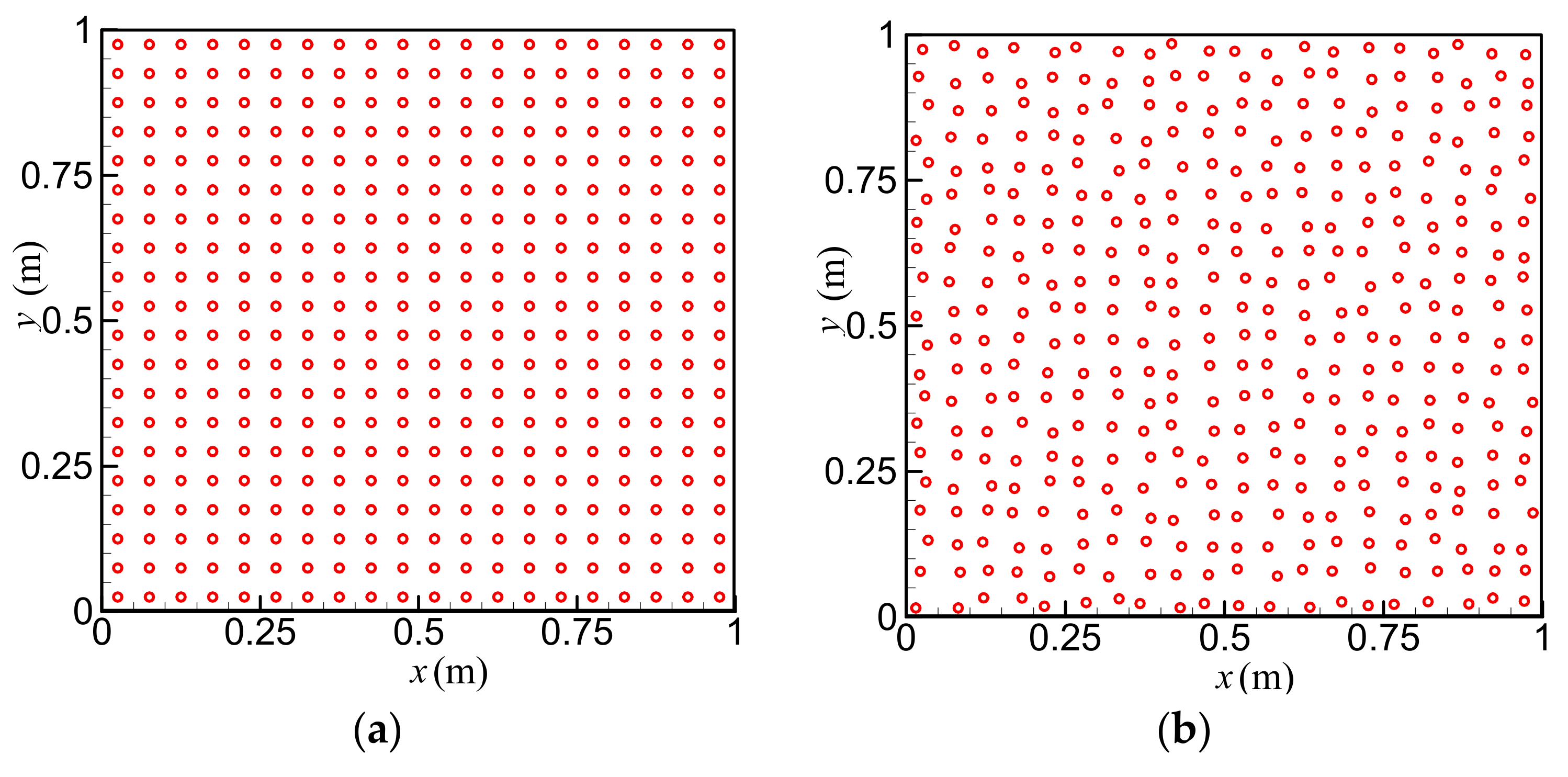
Figure 2.
Comparisons of analytical and numerical results computed by using different viscosity force models with the uniform particle distribution: (a) VISC-01; (b) VISC-02; (c) VISC-03; and (d) VISC-04. SPH, Smoothed Particle Hydrodynamics; VISC, Viscosity Force Model.
Figure 2.
Comparisons of analytical and numerical results computed by using different viscosity force models with the uniform particle distribution: (a) VISC-01; (b) VISC-02; (c) VISC-03; and (d) VISC-04. SPH, Smoothed Particle Hydrodynamics; VISC, Viscosity Force Model.
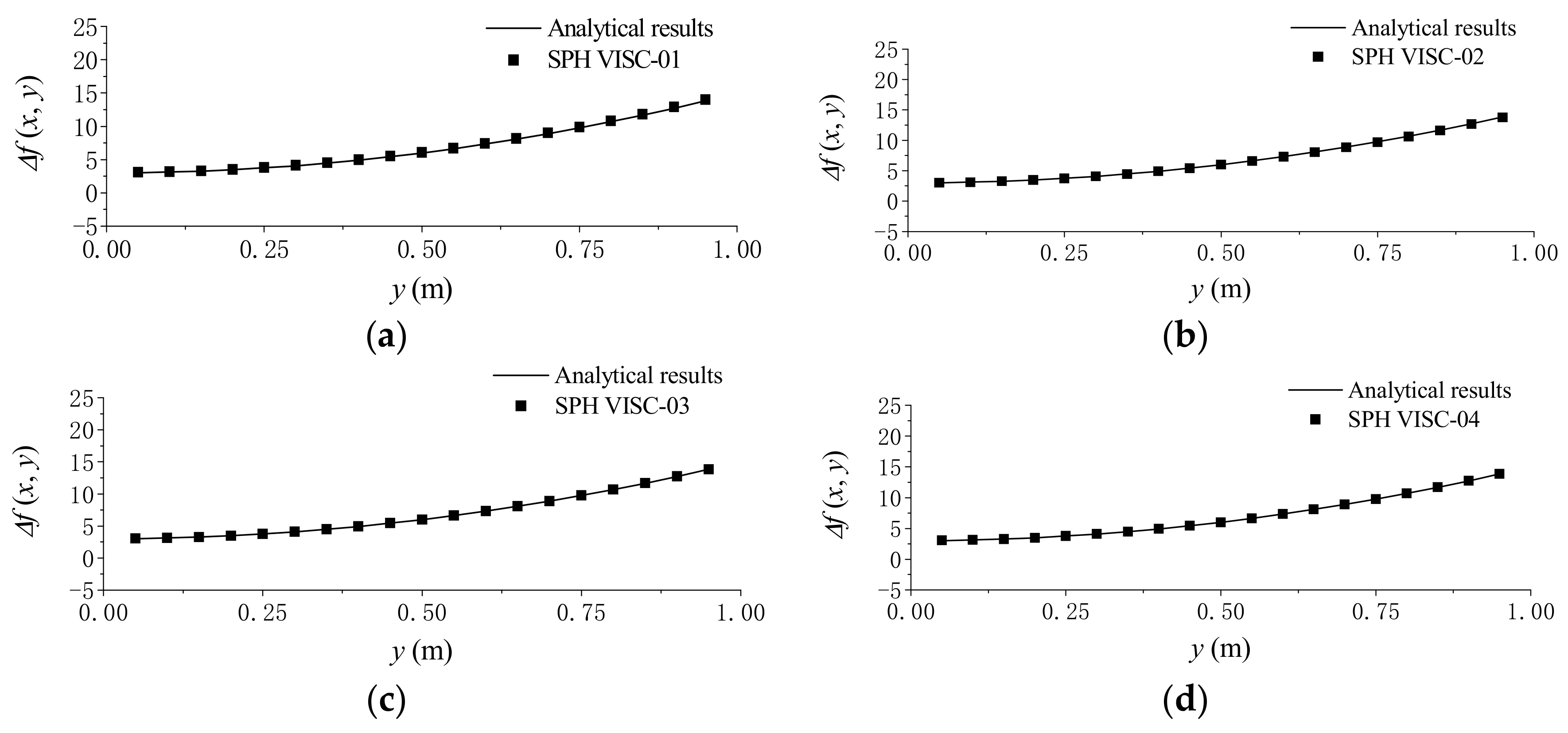
Figure 3.
Convergence and error analysis of different viscosity force models under the uniform particle distribution.
Figure 3.
Convergence and error analysis of different viscosity force models under the uniform particle distribution.
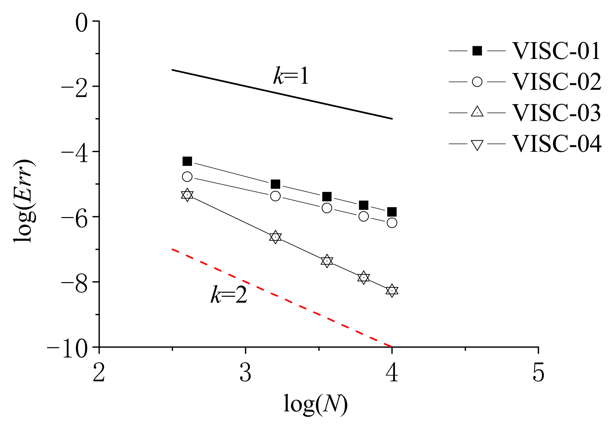
Figure 4.
Comparisons of analytical and numerical results computed by using different viscosity force models with the non-uniform particle distribution: (a) VISC-01; (b) VISC-02; (c) VISC-03; and (d) VISC-04.
Figure 4.
Comparisons of analytical and numerical results computed by using different viscosity force models with the non-uniform particle distribution: (a) VISC-01; (b) VISC-02; (c) VISC-03; and (d) VISC-04.

Figure 5.
Convergence and error analysis of different viscosity force models under the non-uniform particle distribution.
Figure 5.
Convergence and error analysis of different viscosity force models under the non-uniform particle distribution.

Figure 6.
Convergence analysis of CPU time for different viscosity force models under the non-uniform particle distribution.
Figure 6.
Convergence analysis of CPU time for different viscosity force models under the non-uniform particle distribution.

Figure 7.
Vector plots of lid-driven flow for the two different particle numbers: (a) N = 1600; and (b) N = 10,000. Red, location of fluid particle; Black, velocity of flow field.
Figure 7.
Vector plots of lid-driven flow for the two different particle numbers: (a) N = 1600; and (b) N = 10,000. Red, location of fluid particle; Black, velocity of flow field.
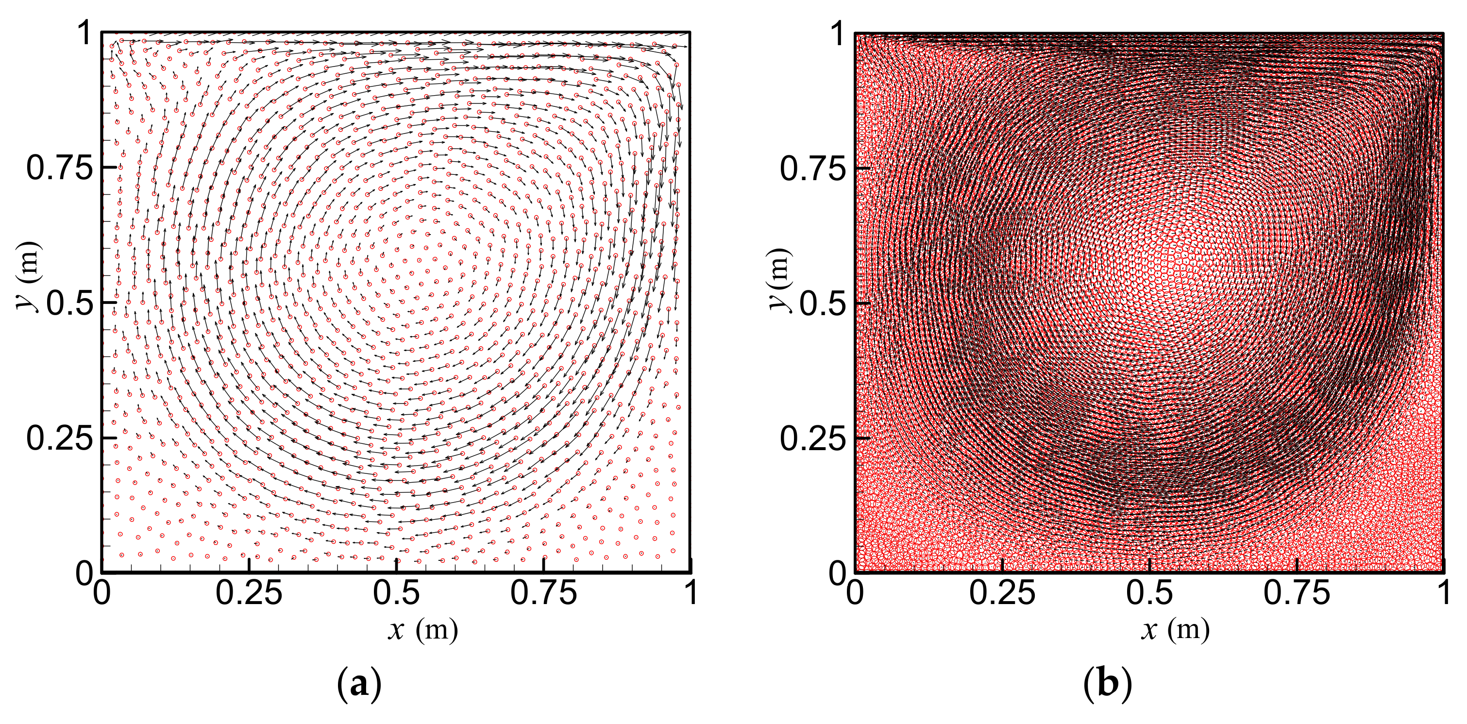
Figure 8.
Velocity amplitude patterns of the lid-driven flow computed by (a) OpenFOAM; and (b) ISPH (VISC-04).
Figure 8.
Velocity amplitude patterns of the lid-driven flow computed by (a) OpenFOAM; and (b) ISPH (VISC-04).
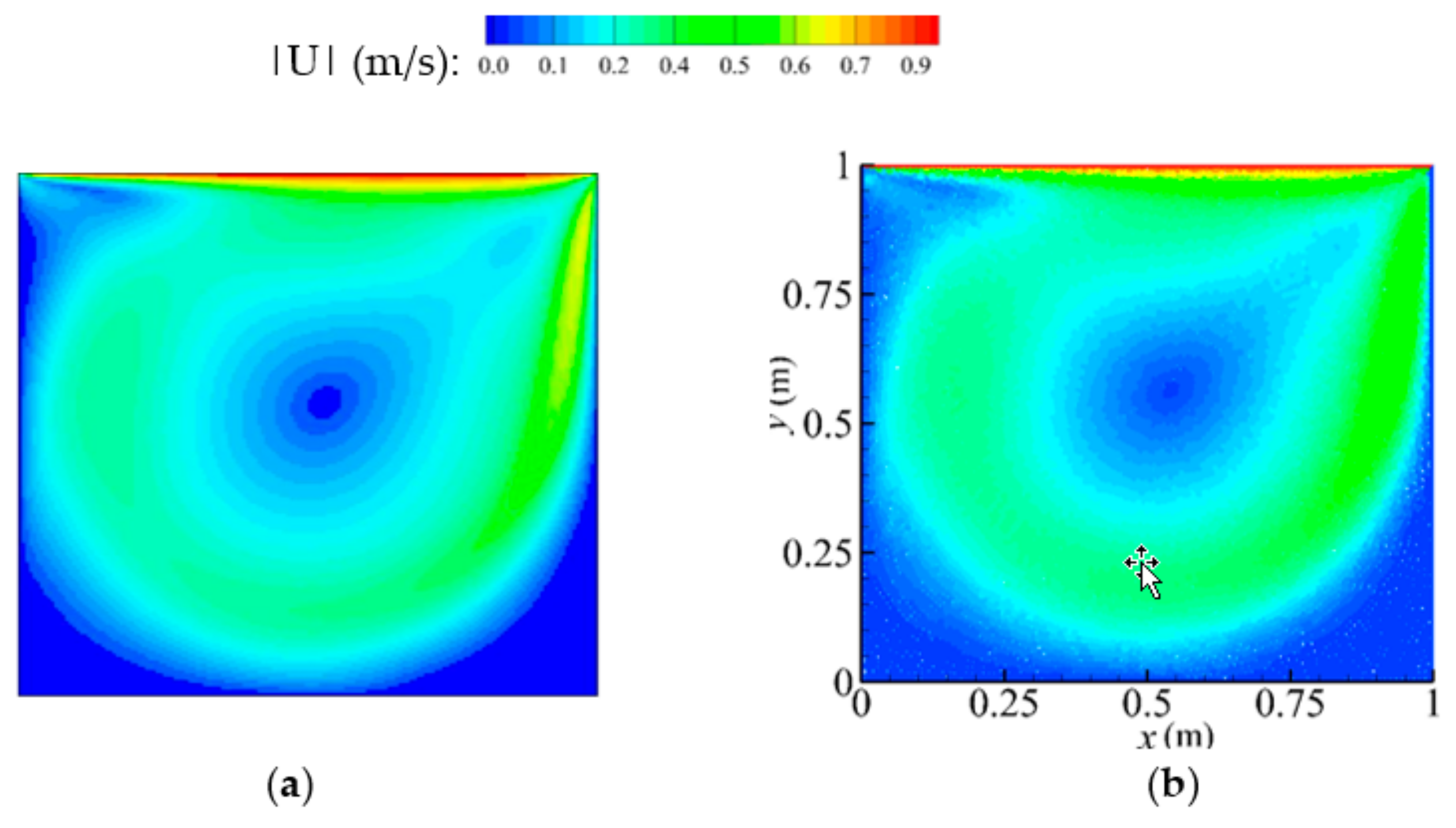
Figure 9.
Comparisons of four viscosity force models for the lid-driven flow: (a) ux velocity distribution; and (b) uy velocity distribution. OpenFOAM, Open source Field Operation and Manipulation; Exp, Experimental data of Ghia et al.
Figure 9.
Comparisons of four viscosity force models for the lid-driven flow: (a) ux velocity distribution; and (b) uy velocity distribution. OpenFOAM, Open source Field Operation and Manipulation; Exp, Experimental data of Ghia et al.

Figure 10.
Convergence and error analysis of four viscosity force models for the different particle resolutions of a lid-driven flow.
Figure 10.
Convergence and error analysis of four viscosity force models for the different particle resolutions of a lid-driven flow.

Figure 11.
(a) Schematic setup of the lid-driven flow model with a cylinder inside; and (b) Velocity vector plot of the cavity flow at time t = 40 s. Red, location of fluid particle; Black, velocity of flow field.
Figure 11.
(a) Schematic setup of the lid-driven flow model with a cylinder inside; and (b) Velocity vector plot of the cavity flow at time t = 40 s. Red, location of fluid particle; Black, velocity of flow field.

Figure 12.
Velocity amplitude patterns of the lid-driven flow with an inside cylinder computed by: (a) OpenFOAM; and (b) ISPH (VISC-04).
Figure 12.
Velocity amplitude patterns of the lid-driven flow with an inside cylinder computed by: (a) OpenFOAM; and (b) ISPH (VISC-04).

Figure 13.
Comparisons of four viscosity force models for the lid-driven flow with an inside cylinder: (a) ux velocity distribution; and (b) uy velocity distribution.
Figure 13.
Comparisons of four viscosity force models for the lid-driven flow with an inside cylinder: (a) ux velocity distribution; and (b) uy velocity distribution.

Figure 14.
Convergence and error analysis of four viscosity force models for the different particle resolutions of a lid-driven flow with an inside cylinder.
Figure 14.
Convergence and error analysis of four viscosity force models for the different particle resolutions of a lid-driven flow with an inside cylinder.


Table 1.
Mean errors with different particle numbers and viscosity calculation methods under the uniform particle distribution. VISC, Viscosity Force Model.
Table 1.
Mean errors with different particle numbers and viscosity calculation methods under the uniform particle distribution. VISC, Viscosity Force Model.
| Particle No. | VISC-01 | VISC-02 | VISC-03 | VISC-04 |
|---|---|---|---|---|
| 20 × 20 | 5.00 × 10⁻⁵ | 1.68 × 10⁻⁵ | 4.65 × 10⁻⁶ | 4.65 × 10⁻⁶ |
| 40 × 40 | 9.81 × 10⁻⁶ | 4.24 × 10⁻⁶ | 2.37 × 10⁻⁷ | 2.37 × 10⁻⁷ |
| 60 × 60 | 4.08 × 10⁻⁶ | 1.84 × 10⁻⁶ | 4.38 × 10⁻⁸ | 4.38 × 10⁻⁸ |
| 80 × 80 | 2.22 × 10⁻⁶ | 1.02 × 10⁻⁶ | 1.34 × 10⁻⁸ | 1.34 × 10⁻⁸ |
| 100 × 100 | 1.40 × 10⁻⁶ | 6.45 × 10⁻⁶ | 5.39 × 10⁻⁹ | 5.39 × 10⁻⁹ |
Table 2.
Mean errors with different particle numbers and viscosity calculation methods under the non-uniform particle distribution.
Table 2.
Mean errors with different particle numbers and viscosity calculation methods under the non-uniform particle distribution.
| Particle No. | VISC-01 | VISC-02 | VISC-03 | VISC-04 |
|---|---|---|---|---|
| 20 × 20 | 2.79 × 10⁻³ | 1.32 × 10⁻³ | 5.62 × 10⁻⁵ | 2.84 × 10⁻³ |
| 40 × 40 | 1.25 × 10⁻³ | 5.85 × 10⁻⁴ | 1.18 × 10⁻⁵ | 1.28 × 10⁻³ |
| 60 × 60 | 8.41 × 10⁻⁴ | 3.80 × 10⁻⁴ | 5.25 × 10⁻⁶ | 8.68 × 10⁻⁴ |
| 80 × 80 | 6.04 × 10⁻⁴ | 2.94 × 10⁻⁴ | 2.90 × 10⁻⁶ | 6.20 × 10⁻⁴ |
| 100 × 100 | 4.72 × 10⁻⁴ | 2.27 × 10⁻⁴ | 1.82 × 10⁻⁶ | 4.85 × 10⁻⁴ |
Table 3.
Comparisons of CPU time with different particle numbers and viscosity calculation methods under the non-uniform particle distribution (unit: s).
Table 3.
Comparisons of CPU time with different particle numbers and viscosity calculation methods under the non-uniform particle distribution (unit: s).
| Particle No. | VISC-01 | VISC-02 | VISC-03 | VISC-04 |
|---|---|---|---|---|
| 20 × 20 | 0.089 | 0.074 | 0.204 | 0.179 |
| 40 × 40 | 0.382 | 0.307 | 0.850 | 0.741 |
| 60 × 60 | 0.900 | 0.739 | 1.976 | 1.719 |
| 80 × 80 | 1.526 | 1.269 | 3.500 | 3.024 |
| 100 × 100 | 2.444 | 1.987 | 5.493 | 4.722 |
© 2018 by the authors. Licensee MDPI, Basel, Switzerland. This article is an open access article distributed under the terms and conditions of the Creative Commons Attribution (CC BY) license (http://creativecommons.org/licenses/by/4.0/).
Share and Cite
MDPI and ACS Style
Zheng, X.; Ma, Q.; Shao, S. Study on SPH Viscosity Term Formulations. Appl. Sci. 2018, 8, 249. https://doi.org/10.3390/app8020249
AMA Style
Zheng X, Ma Q, Shao S. Study on SPH Viscosity Term Formulations. Applied Sciences. 2018; 8(2):249. https://doi.org/10.3390/app8020249
Chicago/Turabian StyleZheng, Xing, Qingwei Ma, and Songdong Shao. 2018. "Study on SPH Viscosity Term Formulations" Applied Sciences 8, no. 2: 249. https://doi.org/10.3390/app8020249
Note that from the first issue of 2016, this journal uses article numbers instead of page numbers. See further details here.