Investigation of Pear Drying Performance by Different Methods and Regression of Convective Heat Transfer Coefficient with Support Vector Machine

1
Vocation High School of Ilic Dursun Yildirim, Erzincan University, Ilic, Erzincan 24700, Turkey
2
Mechanical Engineering, Faculty of Engineering, Firat University, Elazig 23200, Turkey
*
Author to whom correspondence should be addressed.
Appl. Sci. 2018, 8(2), 215; https://doi.org/10.3390/app8020215
Submission received: 14 December 2017
/
Revised: 26 January 2018
/
Accepted: 29 January 2018
/
Published: 31 January 2018
(This article belongs to the Section Mechanical Engineering)
Abstract
:In this study, an air heated solar collector (AHSC) dryer was designed to determine the drying characteristics of the pear. Flat pear slices of 10 mm thickness were used in the experiments. The pears were dried both in the AHSC dryer and under the sun. Panel glass temperature, panel floor temperature, panel inlet temperature, panel outlet temperature, drying cabinet inlet temperature, drying cabinet outlet temperature, drying cabinet temperature, drying cabinet moisture, solar radiation, pear internal temperature, air velocity and mass loss of pear were measured at 30 min intervals. Experiments were carried out during the periods of June 2017 in Elazig, Turkey. The experiments started at 8:00 a.m. and continued till 18:00. The experiments were continued until the weight changes in the pear slices stopped. Wet basis moisture content (MCw), dry basis moisture content (MCd), adjustable moisture ratio (MR), drying rate (DR), and convective heat transfer coefficient (hc) were calculated with both in the AHSC dryer and the open sun drying experiment data. It was found that the values of hc in both drying systems with a range 12.4 and 20.8 W/m2 °C. Three different kernel models were used in the support vector machine (SVM) regression to construct the predictive model of the calculated hc values for both systems. The mean absolute error (MAE), root mean squared error (RMSE), relative absolute error (RAE) and root relative absolute error (RRAE) analysis were performed to indicate the predictive model’s accuracy. As a result, the rate of drying of the pear was examined for both systems and it was observed that the pear had dried earlier in the AHSC drying system. A predictive model was obtained using the SVM regression for the calculated hc values for the pear in the AHSC drying system. The normalized polynomial kernel was determined as the best kernel model in SVM for estimating the hc values.
1. Introduction
The sun is the largest source of carbon-free energy available throughout human history. A lot of research has been done to find out how to use and apply solar energy as a primary energy source [1]. Generally, solar energy application is divided into two basic groups. The first is electricity generation using photovoltaic cells, which convert direct solar energy into electricity, and the other is the thermal application category, which involves solar drying [2].
Drying is defined as a process of removing water from a product and can be applied in two steps. In the first stage, the moisture inside the product is removed to the surface and dried as a water vapor in a constant air. The second stage involves a slow drying rate and the drying process varies according to the type of material to be dried [3]. In sun drying, the product is dried at a high temperature in a closed area or a drying cabinet with the aid of hot air generated in a device known as solar energy and air heater. This drying is an efficient drying process compared to direct sun drying. The product is dried in sun dryer, high temperature and low relative humidity, in comparison with outdoor sun drying. For most agricultural products, a more suitable drying air temperature range is between 45 °C and 60 °C, and between these values the products can be dried by solar and air heating collector systems at varying drying air temperatures [4].
The convective heat transfer coefficient (hc) is an important parameter in drying rate simulation, since the temperature difference between the air and product varies with this coefficient. Akpinar has made to evaluate the convective heat transfer coefficient during drying of various crops and to investigate influence of drying air velocity and temperature on the convective heat transfer coefficient. She has observed that the convective heat transfer coefficient increased in large amount with the increase of the drying air velocity, but increased in small amount with the rise of the drying air temperature [5]. Goyal and Tiwari have studied heat and mass transfer in product drying systems. They have reported the values of convective heat transfer coefficient for wheat and gram as 12.68 and 9.62 W/m2 °C. They have used simple regression and multiple regression technique for predicted the convective heat transfer coefficient [6].
Various predictive models for hc values were established in various systems in the literature. Artificial neural networks are usually used to construct these models [7,8,9,10]. Predictive models of hc values were created by using SVM regression in different topics [11,12]. The use of SVM regression for predicting hc values in food drying systems has not been found in literature. So the SVM regression was chosen for the predictive model.
Recently, SVM regression studies were carried out in various fields. Baser et al. have focused on the estimation of yearly mean daily horizontal global solar radiation by using an approach that utilizes fuzzy regression functions with support vector machine (FRF-SVM). To demonstrate the utility of the FRF-SVM approach in the estimation of horizontal global solar radiation, they have conducted an empirical study over a dataset collected in Turkey and applied the FRF-SVM approach with several kernel functions [13]. Yang at all have investigated the total volatile basic nitrogen (TVB-N) in a total of 210 pork meat pieces (tenderloin) with an average weight of approximately 200–400 g. They have developed Multivariate calibration models using partial least-squares regression (PLSR) and least-squares support vector machines (LS-SVM) in the full spectral range [14]. Li et al. have utilized conventional back propagation neural network (BPNN), radial basis function neural network (RBFNN) general regression neural network (GRNN), and support vector machine (SVM) modeling techniquesfor estimating the hourly cooling load in a building. They used root mean square error (RMSE) and mean relative error (MRE) for estimation of the predictive accuracy of the four models. They have obtained better accuracy and generalization than BPNN and RBFNN methods [15].
In this study, the drying performances between the drying under the sun and the AHSC drying system were compared. Pears were dried in both drying methods. The hc values of pears were calculated in the AHSC drying system and under the sun drying. The SVM regression was applied for the calculated hc coefficients in AHSC drying system. The aim of this study was to establish a predictive model for hc values and to determine which drying method of pears would be faster.
2. Materials and Methods
2.1. Experimental Set-Up
Drying experiment set consisted essentially of an indirect forced convection solar dryer with air heating solar collector panel (1400 mm × 800 mm), a circulation fan and a drying cabinet. Solar air collector panel was made of stainless steel plates (thickness 0.5 mm), the exterior of which was painted with black paint. Solar air heater was covered with copper sheet (thickness, 0.4 mm), which was painted with black collector paint. Glass was used as a transparent cover over the air heater to prevent heat losses. Air heating solar collector was oriented southwards under the collector angle of 23.7° (local latitude 38.4°). The air heating solar collector feet were fixed to this angle. The collector frame was made of stainless steel sheet. Pear drying process under the sun was used in the perforated drying tray (45 cm × 45 cm). Experimental setup is shown in Figure 1.
The pear drying cabinet was made of aluminum material (thickness 2 mm) and designed in rectangular dimensions (100 cm × 50 cm × 100 cm). Spiraled aluminum type pipe was used to transfer the heated air between the collector panel and drying cabinet. Aluminum spiral pipe connections used for hot air transfer between the collector panel and the cabinet were leak-proof. The underside of the cabin was manufactured as hoods to convey hot air from the collector to the cabinet. The drying air in the cabinet was vented from the culvert on the cabin. Three drying trays (90 cm × 40 cm) were placed in the drying cabinet. A circulation fan (0.9 m3/s, 0.4 kW, 220 V, 50 Hz) connected to drying cabinet provides air.
For drying in the AHSC drying system and under the sun, Santa Maria type thin-skinned pears were selected. Selected pears were sliced. Thickness of pear was measured as 10 mm. Solar drying experiments were carried out during the periods of June 2017 in Elazig, Turkey. Experiments were carried out in sunny weather. Test started at 8:00 a.m. and continued till 18:00. Elazig is locate at 38°60′ N and 39°28′ E and above 950 m of sea level in the eastern part of Anatolia, Turkey. In both drying methods, the weight of the pears dried in 30 min periods was measured by digital scale. The experiments were continued until the weight changes in the pear slices stopped. If the weight change continued, the experiments were started again at 8:00 am the next day. During the time when the experiments were not carried out, the mass loss of the orb was neglected. The speed of the air was measured using an anemometer from the air outlet of the drying cabinet. The radiation measurement for the AHSC drying system was made with a pyranometer placed parallel to the solar panel. In the drying under the sun, the pyranometer was placed parallel to the floor and the radiation was measured.
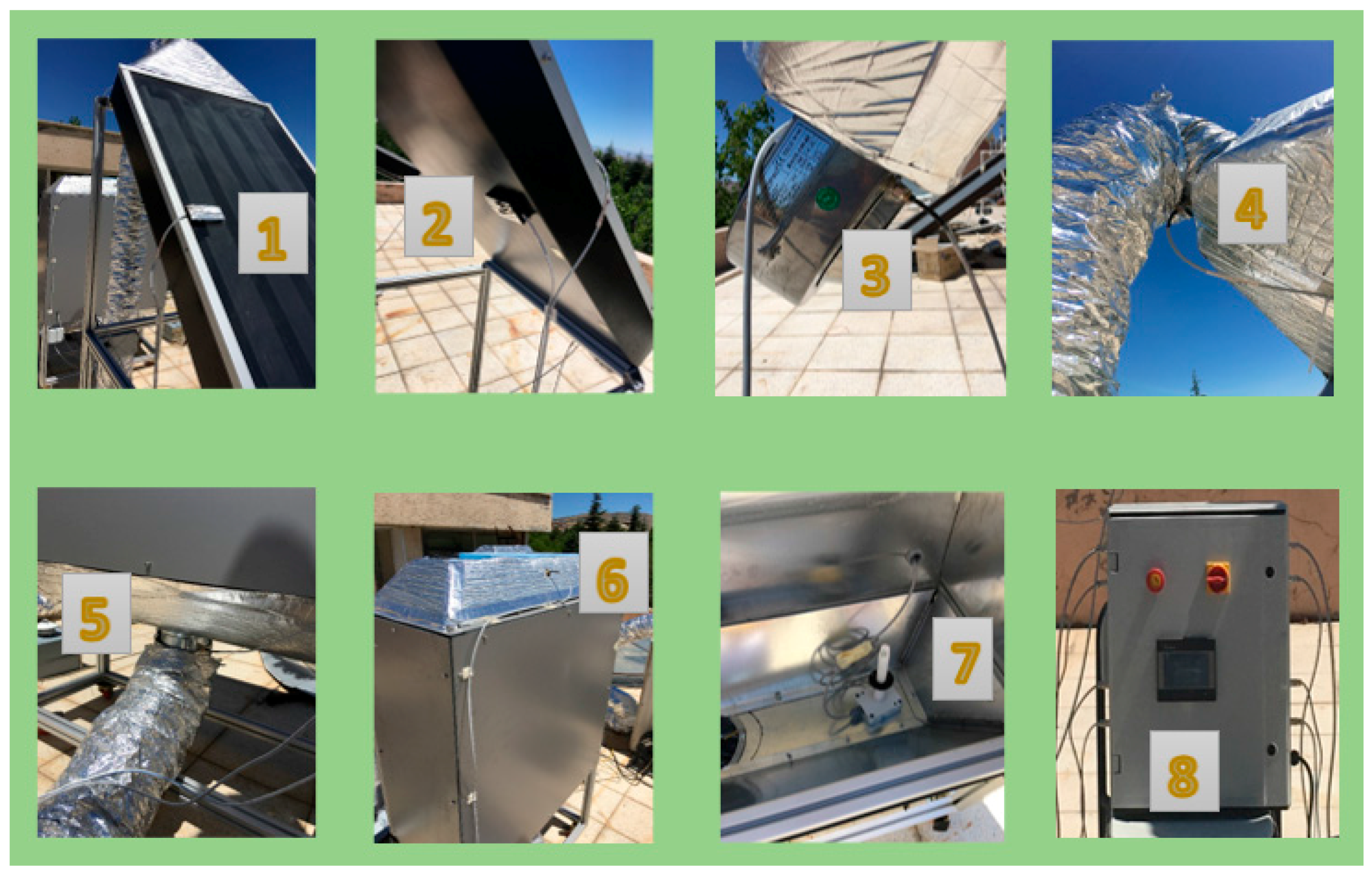
In the experiments, panel inlet temperature, panel outlet temperature, panel glass temperature, panel floor temperature, drying cabinet inlet temperature, drying cabinet outlet temperature, drying cabinet temperature, drying cabinet moisture, solar radiation, drying cabinet air velocity, and mass loss of pear were measured at 30 min intervals. Panel inlet temperature, panel outlet temperature, panel glass temperature, panel floor, temperature, drying cabinet inlet temperature, drying cabinet outlet temperature, drying cabinet temperature and drying cabinet moisture measuring points of AHSC experiment set are presented in Figure 2. Waterproof DS18B20 digital temperature sensors were used for these measuring points.
In the measurements of air temperature (Te) and pear surface temperature (Ts), J type iron-constantan thermocouples were used with a manually controlled 20-channel automatic digital thermometer (ELIMKO, 6400), with reading accuracy of ±0.1 °C. Drying cabinet air velocity was measured by a 0–15 m/s range anemometer (LUTRON, AM-4201), with reading accuracy of ±0.1 m/s. Mass loss of pears were measured during drying by digital balance (BEL, Mark 3100, Monza, Italy) in the measurement range of 0–3100 g and an accuracy of ±0.01 g. The solar radiation during the operation period of drying system was measured with a Kipp and Zonen pyrometer in ±0.1 W/m2 accuracy and its CC12 model digital solar integrator. The initial and final moisture content of mushrooms was determined at 80 °C by Unibloc moisture analyzer (Shimadzu MOC63u) in ±0.001 g accuracy.
2.2. System Analyis
Some general equations used in the drying analysis of the system are given below. For the values of moisture content according to dry basis (MDd) and wet basis (MCw) in pear Equations (1) and (2) have been used.
In Equations (1) and (2); WW is wet weight and DW is dry weight.
Adjustable moisture ratio (MR) values have been calculated using Equation (3).
Drying speed (DR) values have been calculated from Equation (4).
In Equations (3) and (4); M is moisture, Me is equilibrium moisture, Mo is first moisture, “Mt+dt” is moisture content at “t + dt” and Mt is moisture content at “t”.
Convective heat transfer occurs between a moving fluid and solid surface. In this study, it is investigated convective heat transfer for forced convection flow over a flat plate. The viscosity of the fluid requires that the fluid have zero velocity at the plate’s surface. Because a boundary layer exists, the flow is initially laminar but can proceed to turbulence once the Reynolds number of the flow is sufficiently high [16].
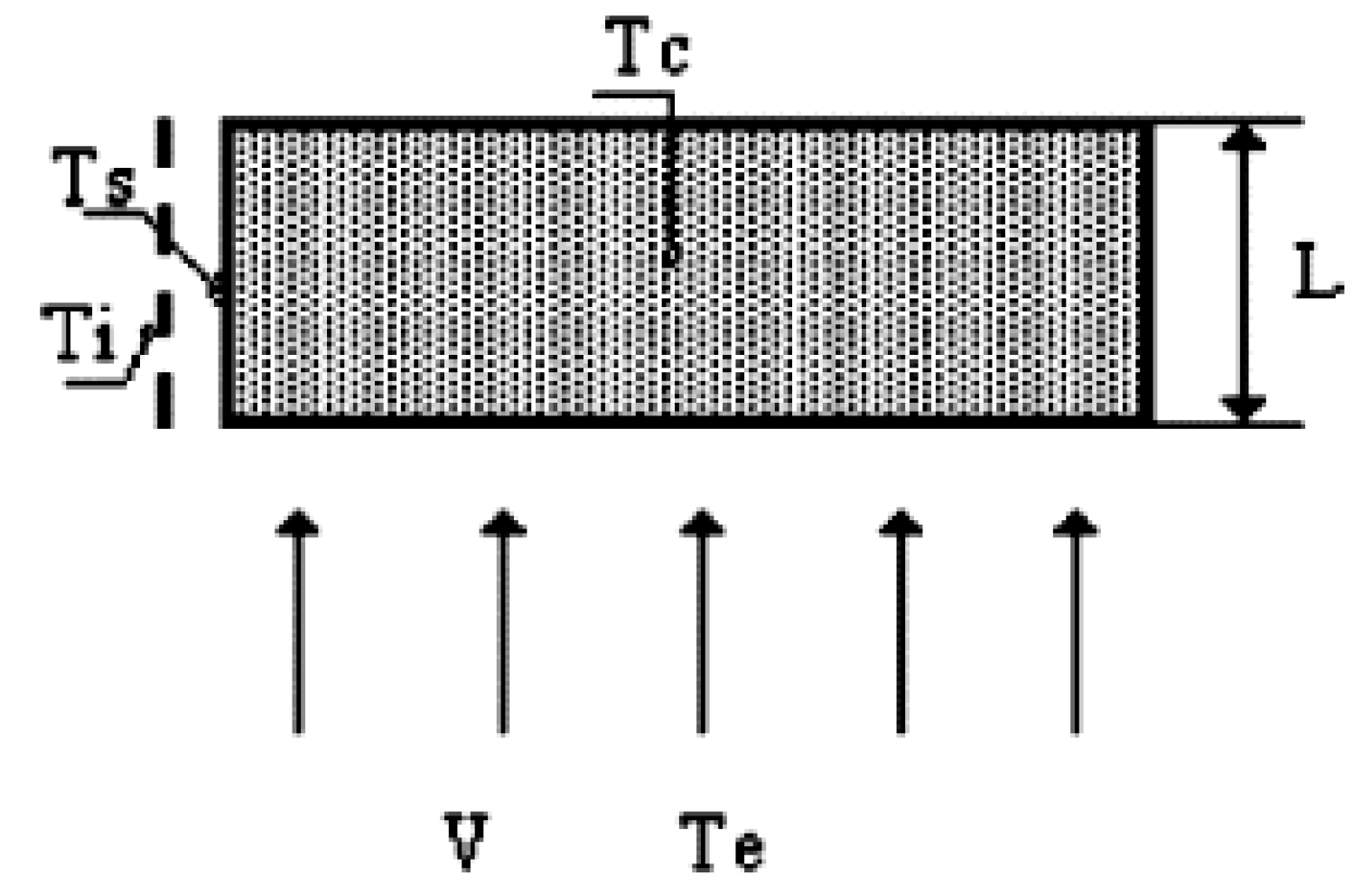
It was assumed that the plate length (L) was sufficiently short so that turbulent flow was never triggered. Air velocity (V), air temperature (Te), central temperature (Tc) and pear surface temperature (Ts) in the drying cabinet are shown in Figure 3. The plate length (pear product thickness) was selected as 0.01 m.
Average heat transfer coefficient was calculated using Pohllhausen Equation (5) for laminar flow and other Equations (6)–(8) that are given below [17]:
The different physical properties of humid air, i.e., density (ρv), thermal conductivity (Kv), specific heat (Cv) and viscosity (µv), used in the computation of Reynolds number (Re) and Prandtl number (Pr) have been determined using the following polynomial expressions [18,19,20]. For obtaining physical properties of humid air Equations (9)–(12) have been used.
Here, Ti was taken as average of product surface temperature (Ts) and drying cabinet air temperature (Te) [18,19,20]:
Akpinar [5] and Velic [17] conceded that turbulence flow does not occur because of the plate length being short in convective heat transfer coefficient (hc) calculations. They calculated the number of hc by the number of Nu. In this study, the Re number for the flow on the plate (pear sample) was calculated at the range of 112.8–132.3 using Equation (7) according to the air velocity and Ti temperature values. According to the obtained Re values, the flow on the plate was accepted as laminar. Using Equation (9), the number of Pr was calculated. In Re and Pr calculations, Equations (9), (11) and (12) obtained with Ti values were used. In Equation (5), the numbers of Re and Pr calculated for the Nu number were used. The Nu value calculated for the laminar flow was used in Equation (6) to calculate the number of hc.
2.3. Regression
The main purpose of the regression analysis is to explain the relationship between dependent variable and independent variable (s) with a mathematical equation. The regression analysis used in the analysis of quantitative variables in general is divided into simple and multiple. Multiple regression analysis, which tends to relate between a dependent variable and a number of independent variables, is a natural extension of simple regression analysis that includes an independent variable. However, multiple regression analysis is more difficult than simple regression analysis. In particular, if there are too many independent variables, it is not possible to draw a graph with more than three dimensions, either directly to the data or to the model [21].
In this study, linear regression has been applied with SVM for hc values. The general formula for linear regression is the following.
In this formula, Y is the dependent variable, ω0 is the regression constant, is the independent variable, and w is the weight of the independent variable.
2.4. Support Vector Machine Regression
Support Vector Machine (SVM) is a classification and regression method that combines theoretical solutions with numerical algorithms. In statistical learning theory, this technique has been developed as a learning algorithm based on Structural Risk Minimization (SRM) rather than Empirical Risk Minimization (ERM). SRM induction principle provides a formal mechanism to determine the optimal model complexity, depending on the Vapnik Chervonenkis (VC) dimension for the finite samples [22]. Compared to classical neural networks, SVM can achieve a single global optimal solution and does not encounter size problems. These attractive features often make SVM a preferred technique. Support vector regression (SVR) is featured with the capability of capturing nonlinear relationship in the feature space and thus is also considered as an effective approach to regression analysis. The following sketches the basic idea of SVR. For more detailed illustration of SVR, please refer to Burges [23].
2.4.1. SVR for Linear Regression
In a regression problem, given a finite data set derived from an unknown function y = g(x) with noise, we need to determine a function y = f(x) solely based on F and to minimize the difference between f and the unknown function g. For linear regression, g is assumed to be a linear relationship between x and y
where x is called feature vector and the space X it lives in is named as feature space. m is the dimension of the feature vector x and the feature space X. y is referred to as the label for each (x,). Now that the relationship to be determined is assumed linear, our goal is to find a hyperplane y = f(x) in the m + 1 dimension space, where are plotted and to minimize the fitting errors by adjusting the parameters. As is proven by Vapnik, the hyperplane is given as
where xk’s are support vectors in the given data set F and yk’s are the corresponding labels. “⋅” represents the inner product in the feature space X. Finding the support vectors and determining the parameters a and b turn out to be α linearly constrained quadratic programming problem that can be solved in multiple ways (e.g., the sequential minimal optimization algorithm [24]. Such a process conducted on the given data set F is called learning. Once the learning phase is done, the model built can be used to predict the corresponding label y from any feature vector x in the feature space X.
2.4.2. SVR for Nonlinear Regression
However, the linear relationship assumption is often too simple to characterize the dynamics of the time series, and thus it is necessary to consider the case when g is nonlinear. The idea of SVR for nonlinear regression is to build a mapping x → φ(x) from the original m dimension feature space X to a new feature space X′ whose dimension depends on the mapping scheme and is not necessarily finite. In the new space X′, the relationship between the new feature vector φ(x) and label y is believed to be in a linear form. By building a proper mapping, the nonlinear relationship can be approximated by doing in the new feature space φ(x) exactly the same thing as is done for the linear case, and it can be proven that the nonlinear version of (2) is
where K(xk, x) = φ(xk) ⋅ φ(x) is the kernel function and “⋅” represents the inner product in the new feature space X′. The new feature φ(x), which can be an infinite dimension vector, is usually not necessary to be computed explicitly, since we normally work with the kernel function in the training and forecasting phases. Accordingly, the kernel function is essential to the performance of SVR [25].
The SVM regression used for the hc values was made by the SMOreg sequence in the Waikato Environment for Knowledge Analysis (WEKA) 3.8.1 program. The WEKA program has been developed at Waikato University. The WEKA Program is open source software and this program supports many algorithms for classification, clustering and association rules. SMOreg implements the support vector machine for regression. The parameters can be learned using various algorithms. The algorithm was selected by setting the RegSMOImproved. The most popular algorithm (RegSMOImproved) is due to Shevade, Keerthi et al. [26].
Various accuracy criteria were used for SVM regression. Accuracy criteria and formulas used in SVM were shown in Table 1.
It is essential to determine the kernel function to be used for a classification operation to be performed by SVM and optimum parameters of this function. The most commonly used radial basis function, Pearson VII (PUK) function and normalized polynomial kernels in the literature are presented together with formulas and parameters in Table 2. As shown in the table, some parameters for each kernel function must be specified by the user.
3. Results and Discussion
In this study, pears were dried in AHSC drying system and outdoors. The initial moisture content of the dried pear slices was determined to be 83.1% (4.9 g water/g solid matter). The drying process was terminated when the moisture transfer between the product and the desiccant media air ended and thus the moisture content remained constant at 21.4% (0.27 g water/g solids).
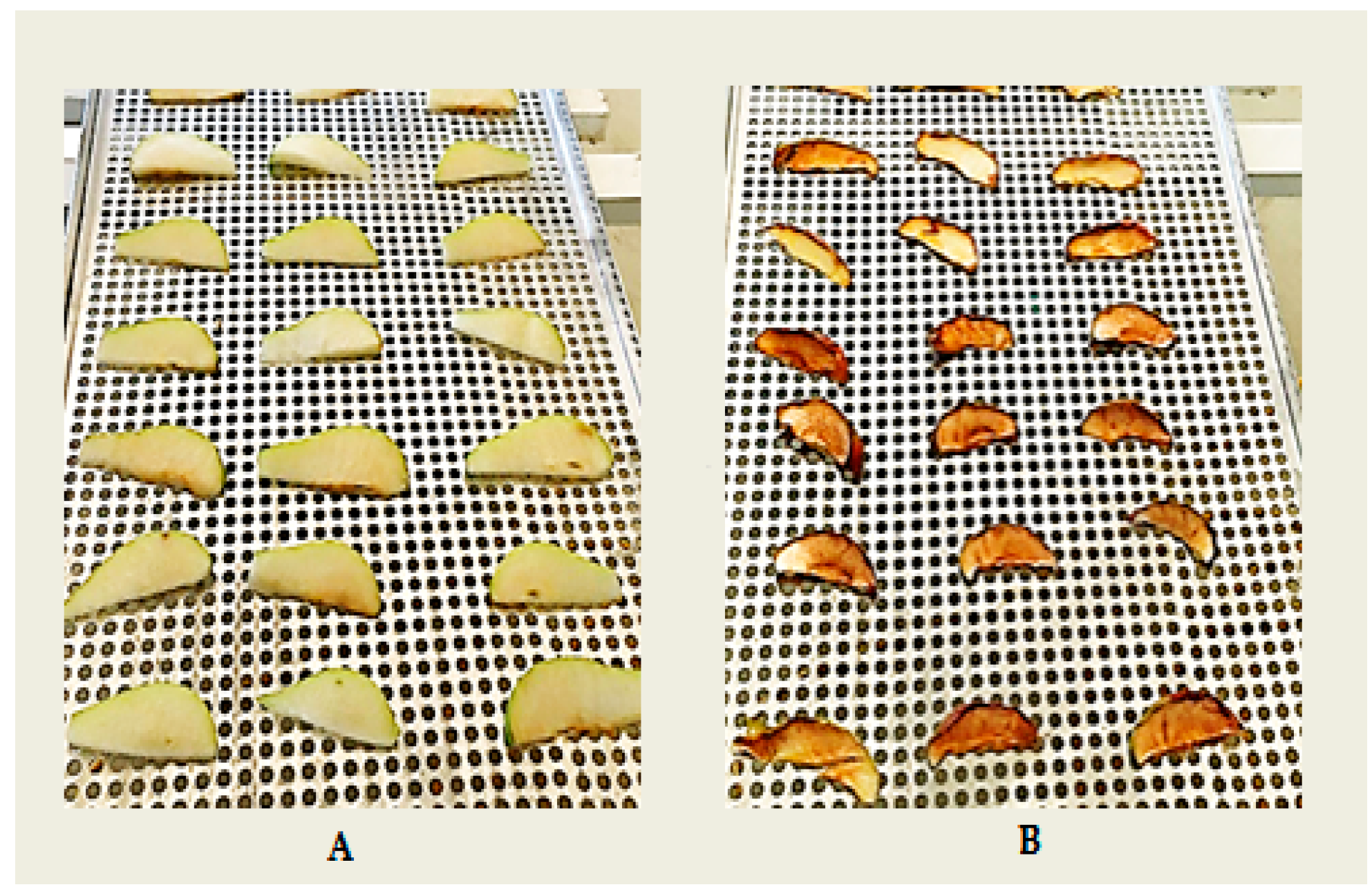
In the drying experiments, the pear slices were started to dry in the AHSC drying system and under the sun, and the experiment was continued in both systems until the moisture content was fixed. The images of pear slices before and after drying are shown in Figure 4.
The experimental data obtained from the AHSC drying system and under the sun drying were shown in Table 3 and Table 4. Pears were weighed together with the drying tray in the weight measurements. Measured product weight was recorded in Table 3 and Table 4 as total weight value minus drying tray weight value. In the Table 3 and Table 4, the 0 value show that the first measurements taken at 8:00 a.m. The 600 value shows that the last measurements taken at 18:00. If the product weight continued to change at 18:00, the experiment was terminated and continued at 08:00 a.m. the next day. According to this, in the AHSC drying system, the experiments were completed in 1 day, while the under sun drying experiments were completed in 2 days.
When outdoor temperatures were measured, there were irregularities due to adverse weather conditions (cloud, wind etc.). In order to remedy these adverse conditions, the outdoor temperature values in the range of 780 and 840 were assumed to be constant in Table 4.
The panel inlet temperature measurement point for the AHSC drying system was shown in Figure 2 as Figure 3. The hood was used to connect the fan with the solar panel. The output temperature of the fan was measured with the help of the sensor installed in the hood. The temperature sensor inside the hood may create a temperature difference of several degrees between The Panel Inlet Temperature in Table 3 and the Outdoor Temperature in Table 4.
The air was sent to the solar collector via the fan with a constant speed. The air heated when it passed through the absorbent plate in solar collector. For this reason, there may be changes in the temperature of the air and the values of drying cabinet air velocity may vary in Table 3 and Table 4.
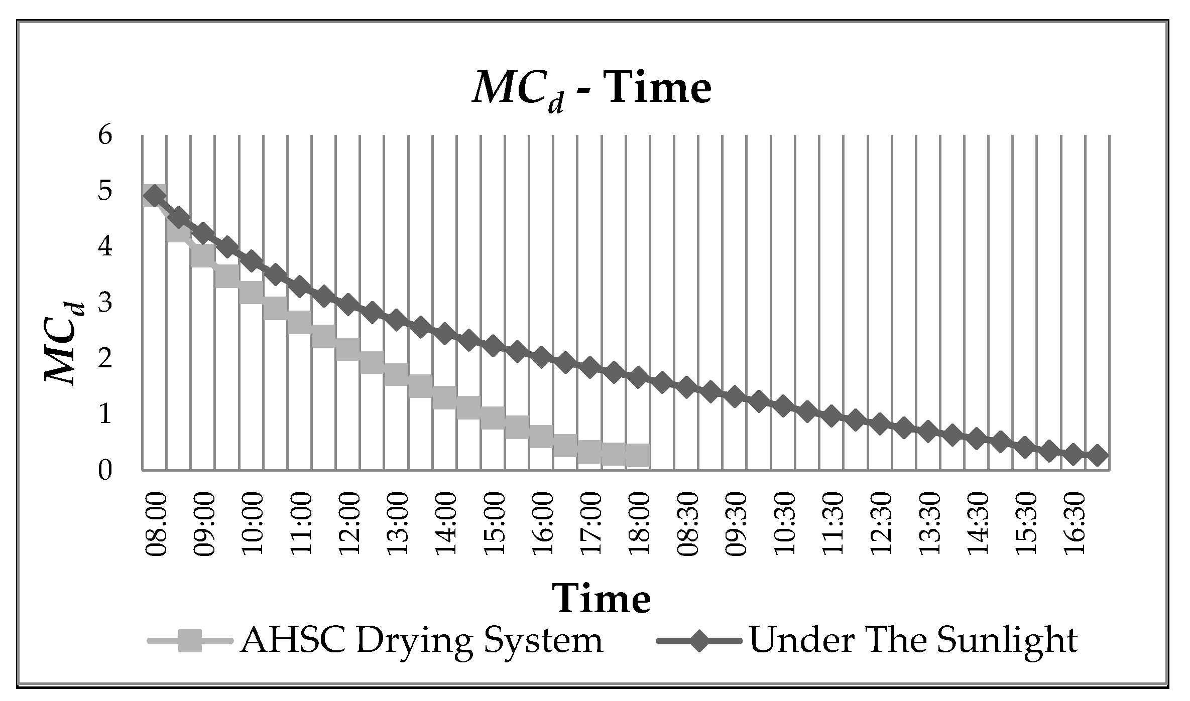
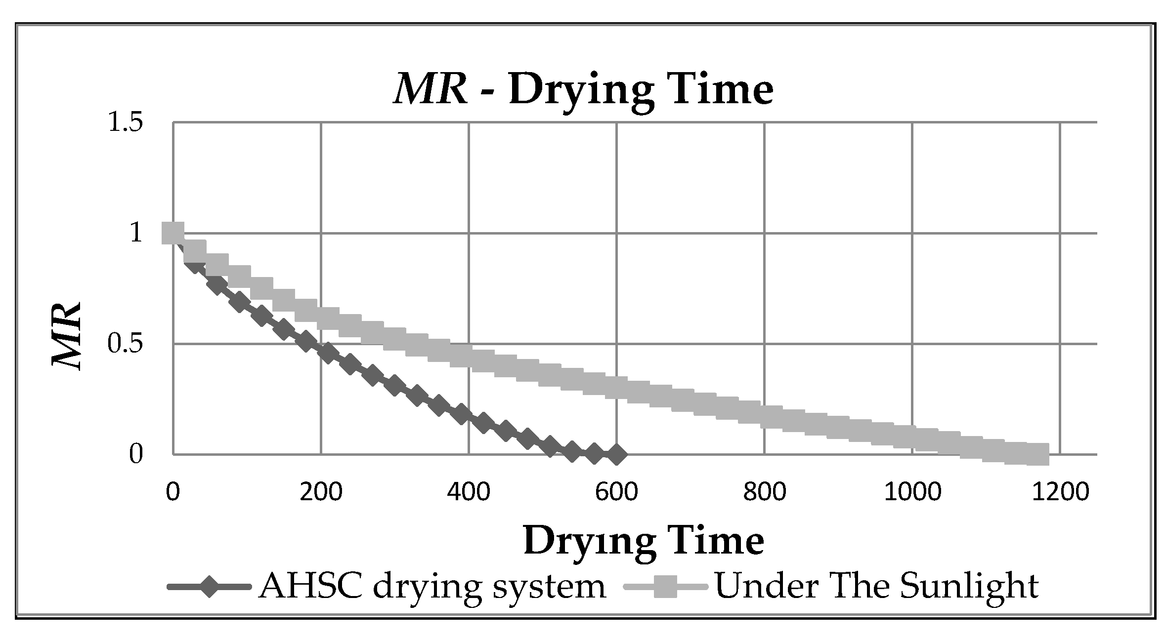
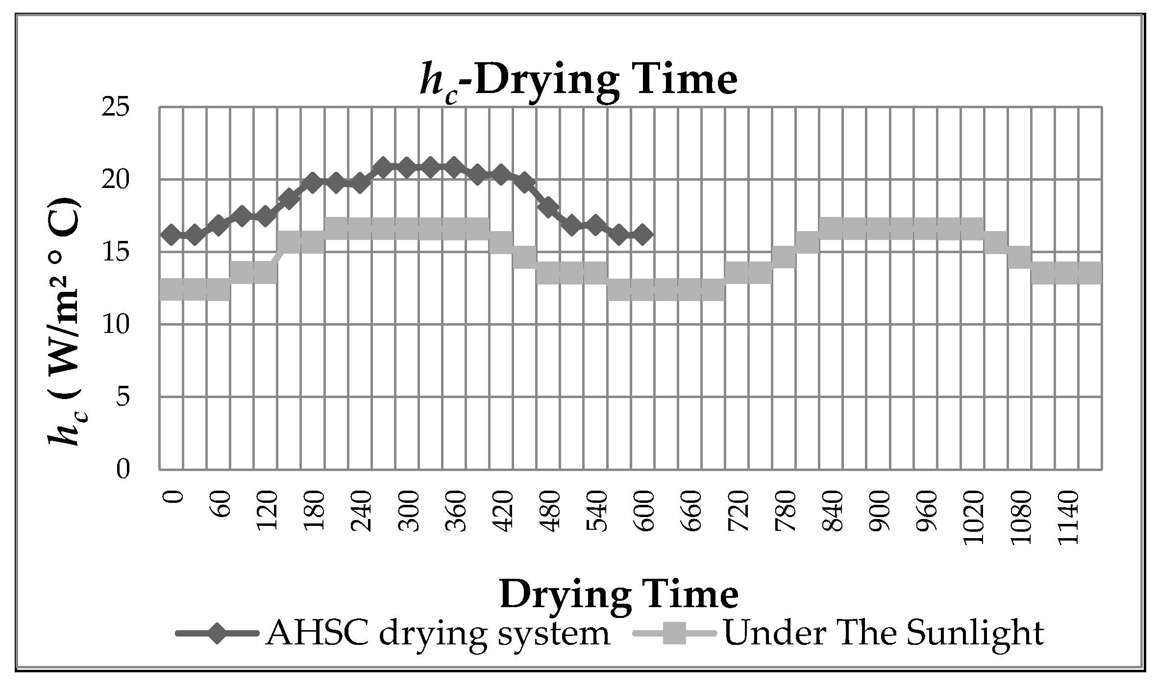
MCd, MR, DR and hc values obtained by Equations (1), (3) and (4) for the AHSC and the open-air drying system dried pears are shown in Figure 5, Figure 6, Figure 7 and Figure 8 respectively. Figure 5, Figure 6, Figure 7 and Figure 8 were added to indicate that the AHSC drying system had better drying performance than the under-sun drying. According to Figure 5, when the moisture content values were examined over time, it was seen that moisture content first decreases in the drying in the AHSC drying system. This indicates that the AHSC drying system was more effective in pear drying. As shown in Figure 6, Figure 7 and Figure 8, drying time in the AHSC drying system was less than drying under the sun. As can be understood from this situation, pears dry in the AHSC drying system earlier than in the sun. According to Figure 8, the value of hc in the AHSC drying system is higher than the value of hc in the sun. This shown that the heat transfer on the dried pear under the sun drying was lower than the AHSC drying system.
In this study, to make choosing an appropriate noise level easier, this implementation applies normalization/standardization to the target attribute as well as the other attributes. Missing values were replaced by the global mean/mode. Nominal attributes were converted to binary ones. We used three kernel models (1—The normalized polynomial kernel; 2—The Pearson VII function-based universal (PUK) kernel; 3—The radial-based function (RBF) kernel) of SVM regression.
18 Attributes (378 data) have been used for SVM Regression. hc (21 data) has been selected to be used as the class. Cross-Validation (Folds = 10) has been used for test options. The mean absolute error (MAE), root mean squared error (RMSE), relative absolute error (RAE) and root relative absolute error (RRAE) values for the 3 kernel models are shown in Table 5.
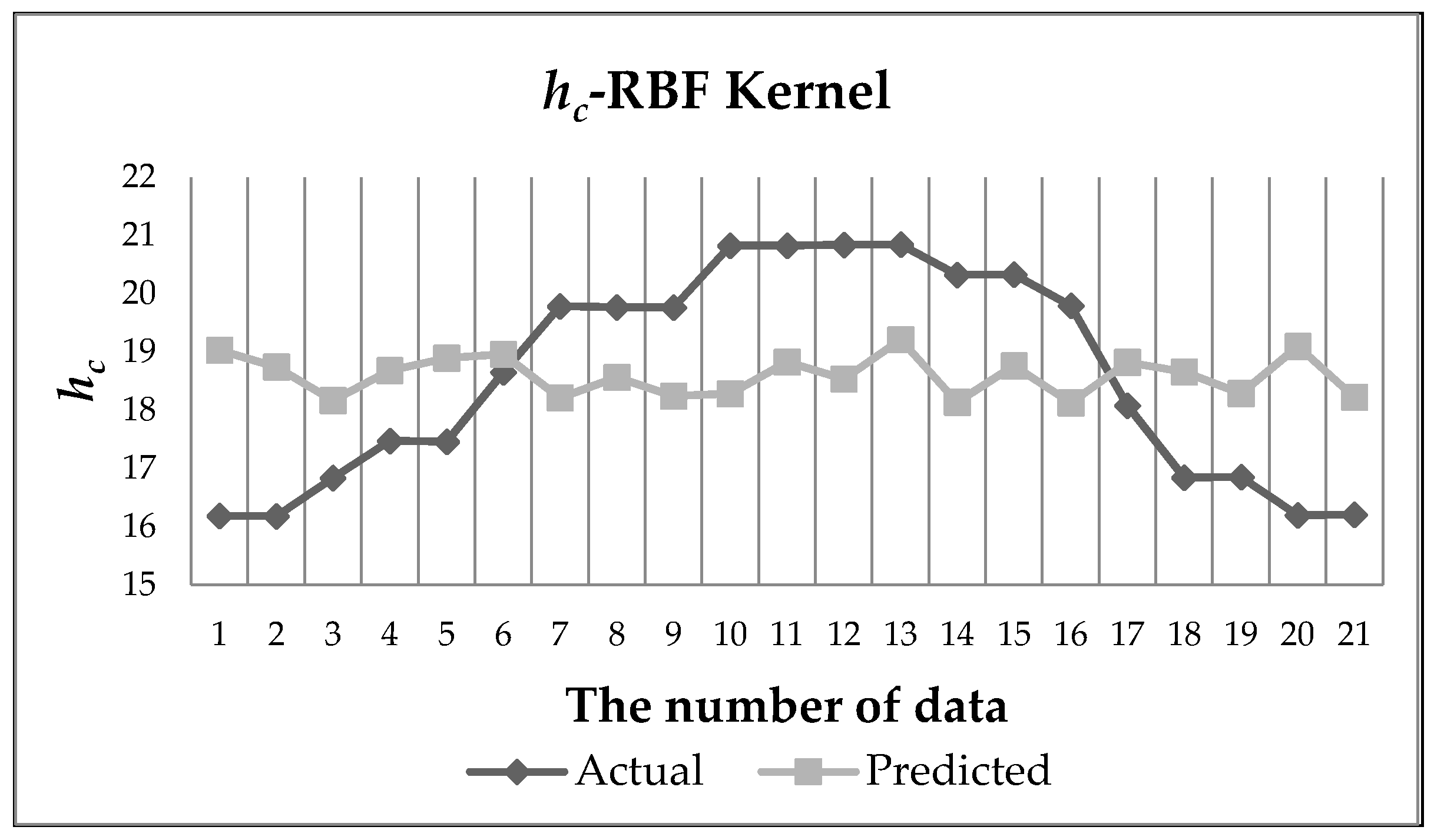
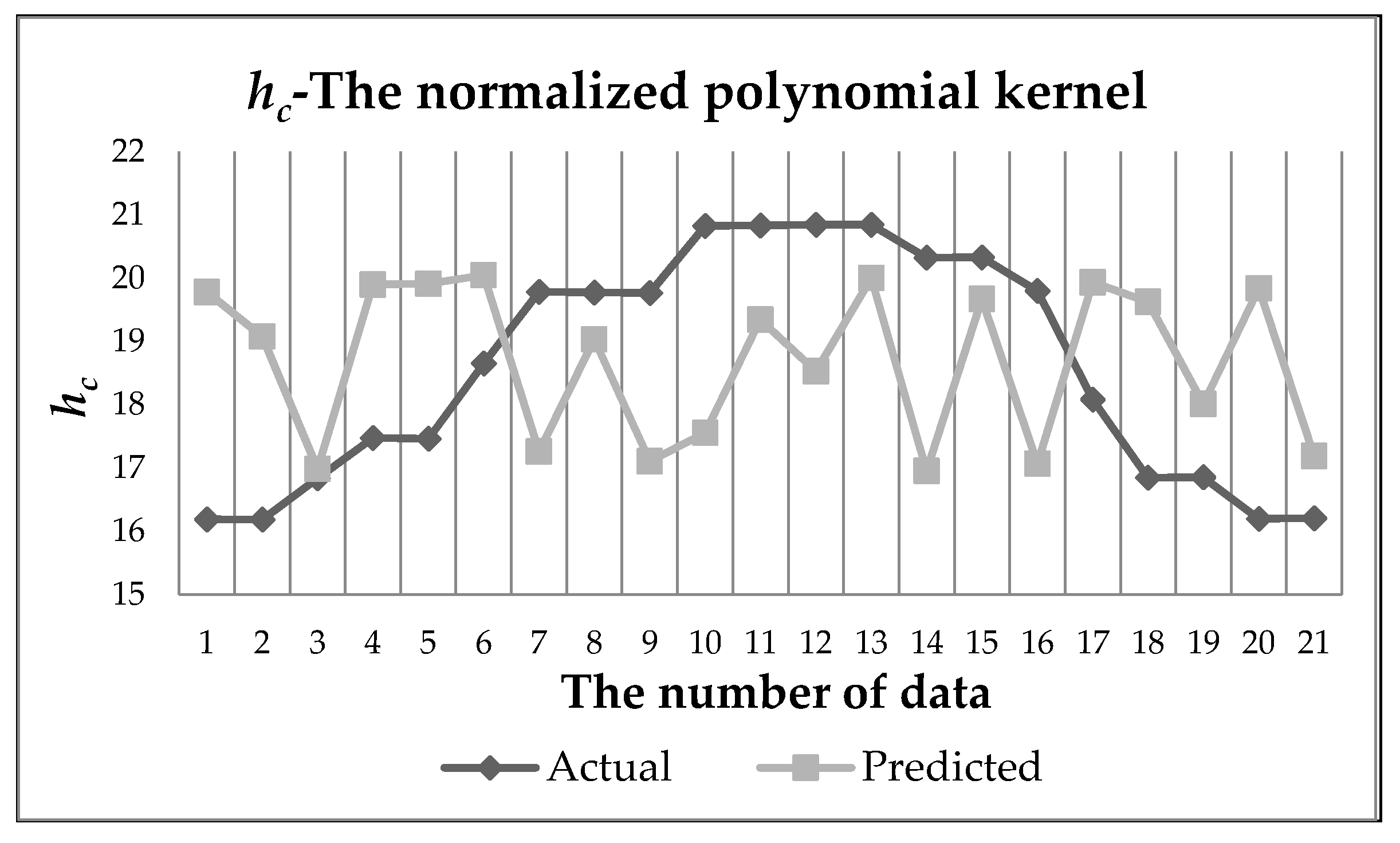
The predicted and actual hc values for each kernel models are shown in Figure 9, Figure 10 and Figure 11. The hc values of pears in the AHSC drying system were modeled and estimated with SVM regression. The kernel model with the least error rates in the SVM regression for the hc values according to Table 5 was normalized polynomial kernels. Figure 9, Figure 10 and Figure 11 show the predicted and actual values for hc values based on 3 different kernel models in the SVM regression. Figure 9 shown that the actual and predicted values were closer to each other.
More efficient results can be obtained when the error rate of the estimated values of the kernel models is small. The error rates are related to the network training used for the SVMreg model. The network can be better trained using more data. In this study, 378 data were used to construct the SVMreg model. As the drying time of the pear product was short, 378 pieces of data were obtained. By using products with longer drying times, more data can be obtained and therefore better predicted values can be obtained.
In the AHSC drying system, hot air sent to the drying cab is provided by the solar panel. Hot air from the panel is sent to the drying cab with the aid of a radial fan. In Table 3, the temperature of the air passing through the panel changes according to the solar radiation values on the solar panel. If the sun rays fall at a right angle to the stationary panel, more warm air is provided. Because the solar panel is fixed, the sun rays do not always come at a right angle. Therefore, the temperature values of the air at the exit of the panel and the hc values for the speed change were calculated between 16.3 and 21.1.
Result of SVM regression for hc values SMOreg function in the WEKA program is given in Table 6 obtained from 3 different kernel functions.
In the above formulas, k is called feature vector and the space K it lives in is named as feature space. The k[n] values are the support vectors corresponding to the hc values estimated by the WEKA program of 21 experimental hc data determined as class.
Various predictive intelligence methods have been used for the heat transfer coefficient. The most common of these methods is ANN. Using SVM is not much. The error statistic values should be low when constructing the predictive model in predictive intelligence methods. A low error rate indicates a high estimate. Verma [8] and Hassampour [9] have developed a predictive model using the ANN for hc value in different systems. Verma and others predicted the heat transfer of concentric tube heat exchanger value using ANN. They achieved root mean square error (RMSE) as 0.354 in predictive model. Hassanpour and others predicted the pool boiling heat transfer coefficient of alumina water-based nanofluids using ANN. They used 870 data for ANN. They found mean square error (MSE) as 4.17 in predictive model. Zaidi [11] predicted the two phase boiling heat transfer coefficient using SVM. He found predictive value of RMSE as 0.581. In this study, the MSE and RMSE values of the predictive model for the heat transfer coefficient using the normalized polynomial kernel in SVM regression are 0.279 and 0.3351. A better predictive model was obtained than the studies given above.
More efficient result may be obtained when parameters of SVM are optimized. Extreme learning machine which is one of the most recent machine learning methods may also be efficiently used for regression of convective heat transfer coefficient problem. Furthermore; when the number of data can be increased by using products with longer drying periods in this system, data mining methods may be utilized for the discovery of valuable knowledge automatically.
4. Conclusions
In conclusion, the pear product was dried in the AHSC drying system and under the sun. The drying behavior of different drying systems of the pear has been examined. The drying performances of these two different drying methods were compared and it was observed that the AHSC drying system performed a more efficient drying.
SVM regression was used for hc values of pear in the AHSC drying system. Using SVM regression, create a predictive model for hc values. We can specify that the best kernel model is the normalized polynomial kernel for estimating the hc values in the SVM regression. We can use the models obtained from SVM regression for hc values in different drying methods.
Acknowledgments
This study was supported by “Firat University Scientific Research Foundation” (Project Numbers 2017-MF.17.11 and 2017-MF 16.54).
Author Contributions
Mehmet Das and Ebru Kavak Akpinar designed the proposed method and experiments; Mehmet Das performed the experiments. Mehmet Das and Ebru Kavak Akpinar wrote the paper.
Conflicts of Interest
The authors declare no conflict of interest.
References
- Barlev, D.; Vidu, R.; Stroeve, P. Innovation in concentrated solar power. Sol. Energy Mater Sol. Cells 2011, 95, 2703–2725. [Google Scholar] [CrossRef]
- Mekhilef, S.; Safari, A.; Mustaffa, W.E.S.; Saidur, R.; Omar, R.; Younis, M.A.A. Solar energy in Malaysia: Current state and prospects. Renew. Sustain. Energy Rev. 2012, 16, 386–396. [Google Scholar] [CrossRef]
- El-Sebaii, A.A.; Shalaby, S.M. Solar drying of agricultural products: A review. Renew. Sustain. Energy Rev. 2012, 16, 37–43. [Google Scholar] [CrossRef]
- Agrawal, A.; Sarviya, R.M. A review of research and development work on solar dryers with heat storage. Int. J. Sustain. Energy 2016, 35, 583–605. [Google Scholar] [CrossRef]
- Akpınar, E.K. Evaluation of convective heat transfer coefficient of various crops in cyclone type dryer. Energy Convers. Manag. 2005, 46, 2439–2454. [Google Scholar] [CrossRef]
- Goyal, R.K.; Tiwari, G.N. Heat and mass transfer relations for crop drying. Dry. Technol. 1998, 16, 1741–1754. [Google Scholar] [CrossRef]
- Acikgoz, O.; Çebi, A.; Dalkilic, A.S.; Koca, A.; Çetin, G.; Gemici, Z.; Wongwises, S. A novel ANN-based approach to estimate heat transfer coefficients in radiant wall heating systems. Energy Build. 2017, 144, 401–415. [Google Scholar] [CrossRef]
- Hassanpour, M.; Vaferi, B.; Masoumi, M.E. Estimation of pool boiling heat transfer coefficient of alumina water-based nanofluids by various artificial intelligence (AI) approaches. Appl. Therm. Eng. 2018, 128, 1208–1222. [Google Scholar] [CrossRef]
- Verma, T.N.; Nashine, P.; Singh, D.V.; Singh, T.S.; Panwar, D. ANN Prediction of an experimental heat transfer analysis of concentric tube heat exchanger with corrugated inner tubes. Appl. Therm. Eng. 2017, 120, 219–227. [Google Scholar] [CrossRef]
- Romero-Méndez, R.; Lara-Vázquez, P.; Oviedo-Tolentino, F.; Durán-García, H.M.; Pérez-Gutiérrez, F.G.; Pacheco-Vega, A. Use of Artificial Neural Networks for Prediction of the Convective Heat Transfer Coefficient in Evaporative Mini-Tubes. Ingeniería, Investigación y Tecnología 2016, 17, 23–34. [Google Scholar] [CrossRef]
- Zaidi, S. Novel application of support vector machines to model the two phase boiling heat transfer coefficient in a vertical tube thermosiphon reboiler. Chem. Eng. Res. Des. 2015, 98, 44–58. [Google Scholar] [CrossRef]
- Gandhi, A.B.; Joshi, J.B. Estimation of heat transfer coefficient in bubble column reactors using support vector regression. Chem. Eng. J. 2010, 160, 302–310. [Google Scholar] [CrossRef]
- Baser, F.; Demirhan, H. A fuzzy regression with support vector machine approach to the estimation of horizontal global solar radiation. Energy 2017, 123, 229–240. [Google Scholar] [CrossRef]
- Yang, Q.; Sun, D.W.; Cheng, W. Development of simplified models for nondestructive hyperspectral imaging monitoring of TVB-N contents in cured meat during drying process. J. Food Eng. 2017, 192, 53–60. [Google Scholar] [CrossRef]
- Li, Q.; Meng, Q.; Cai, J.; Yoshino, H.; Mochida, A. Predicting hourly cooling load in the building: A comparison of support vector machine and different artificial neural networks. Energy Convers. Manag. 2009, 50, 90–96. [Google Scholar] [CrossRef]
- Pitts, D.R.; Sissom, L.E. Schaums’s Outline of Theory and Problems of Heat Transfer; McGraw-Hill Inc.: New York, NY, USA, 1977. [Google Scholar]
- Velic, D.; Planinic, M.; Tomas, S.; Bilic, M. Influence of airflow velocity on kinetics of convection apple drying. J. Food Eng. 2004, 64, 97–102. [Google Scholar] [CrossRef]
- Anwar, S.I.; Tiwari, G.N. Evaluation of convective heat transfer coefficient in crop drying under open sun drying conditions. Energy Convers. Manag. 2001, 42, 627–637. [Google Scholar] [CrossRef]
- Anwar, S.I.; Tiwari, G.N. Convective heat transfer coefficient of crop in forced convection drying-an experimental study. Energy Convers. Manag. 2001, 42, 1687–1698. [Google Scholar] [CrossRef]
- Tiwari, G.N. Solar Energy, Fundamentals, Design, Modelling and Applications; Alpha Science International Ltd.: Oxford, UK, 2002. [Google Scholar]
- Kleınbaum, D.C.; Kupper, L.C.; Muller, K.E. Applied Regression Analysis and Other Multivariable Methods; PWS-KENT Publishing Co.: Boston, MA, USA, 1988; ISBN 0-87150-123-6. [Google Scholar]
- Vapnik, V. The Nature of Statistical Learning Theory; Springer: Berlin, Germany, 1995. [Google Scholar]
- Burges, C.J.C. A tutorial on support vector machines for pattern recognition. Data Min. Knowl. Discov. 1998, 2, 121–167. [Google Scholar] [CrossRef]
- Schölkopf, B.; Burges, C.J.C.; Smola, A.J. Advances in Kernel Methods: Support Vector Learning; MIT Press: Cambridge, MA, USA, 1999. [Google Scholar]
- Qu, H.; Zhang, Y. A New Kernel of Support Vector Regression for Forecasting High-Frequency Stock Returns. Math. Probl. Eng. 2016, 2016, 4907654. [Google Scholar] [CrossRef]
- Shevade, S.K.; Keerthi, S.S.; Bhattacharyya, C.; Murthy, K.R.K. Improvements to the SMO Algorithm for SVM Regression. IEEE Trans. Neural Netw. 1999, 11, 1188–1193. [Google Scholar] [CrossRef] [PubMed]
Figure 1.
Experimental set-up: (1) drying cabinet; (2) solar collector; (3) circulation fan; (4) pear drying under the sun.
Figure 1.
Experimental set-up: (1) drying cabinet; (2) solar collector; (3) circulation fan; (4) pear drying under the sun.
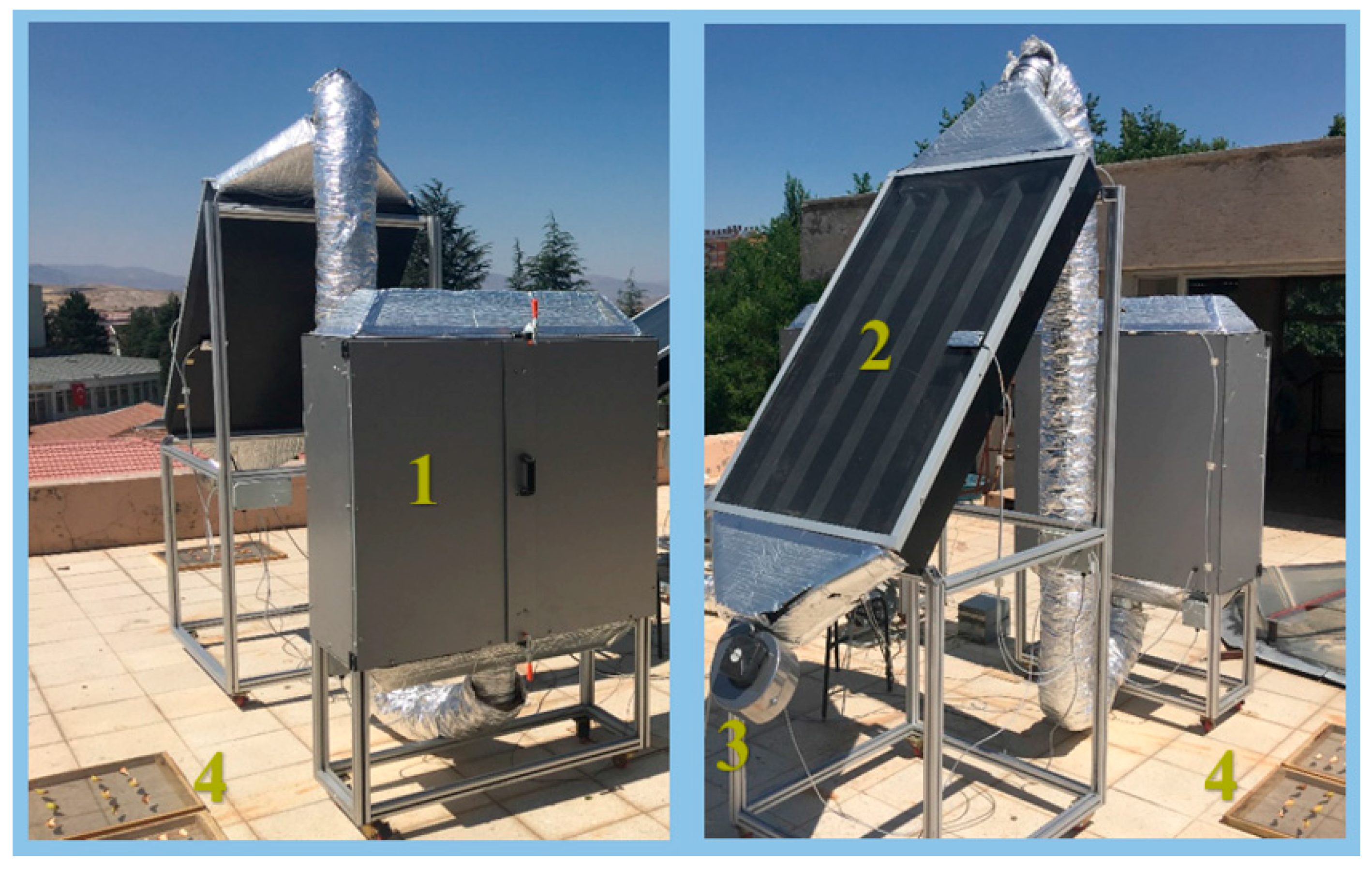
Figure 2.
The measuring points: (1) Panel glass temperature; (2) panel floor temperature; (3) panel inlet temperature; (4) panel outlet temperature; (5) drying cabinet inlet temperature; (6) drying cabinet outlet temperature; (7) drying cabinet temperature; (8) measurement monitoring screen.
Figure 2.
The measuring points: (1) Panel glass temperature; (2) panel floor temperature; (3) panel inlet temperature; (4) panel outlet temperature; (5) drying cabinet inlet temperature; (6) drying cabinet outlet temperature; (7) drying cabinet temperature; (8) measurement monitoring screen.

Figure 3.
Convection heat transfer for forced flow over a flat plate.

Figure 4.
Before and after the drying process pear images: (A) before drying; (B) after drying.

Figure 5.
MCd changing with time.

Figure 6.
MR changing with drying time.

Figure 7.
DR changing with drying time.
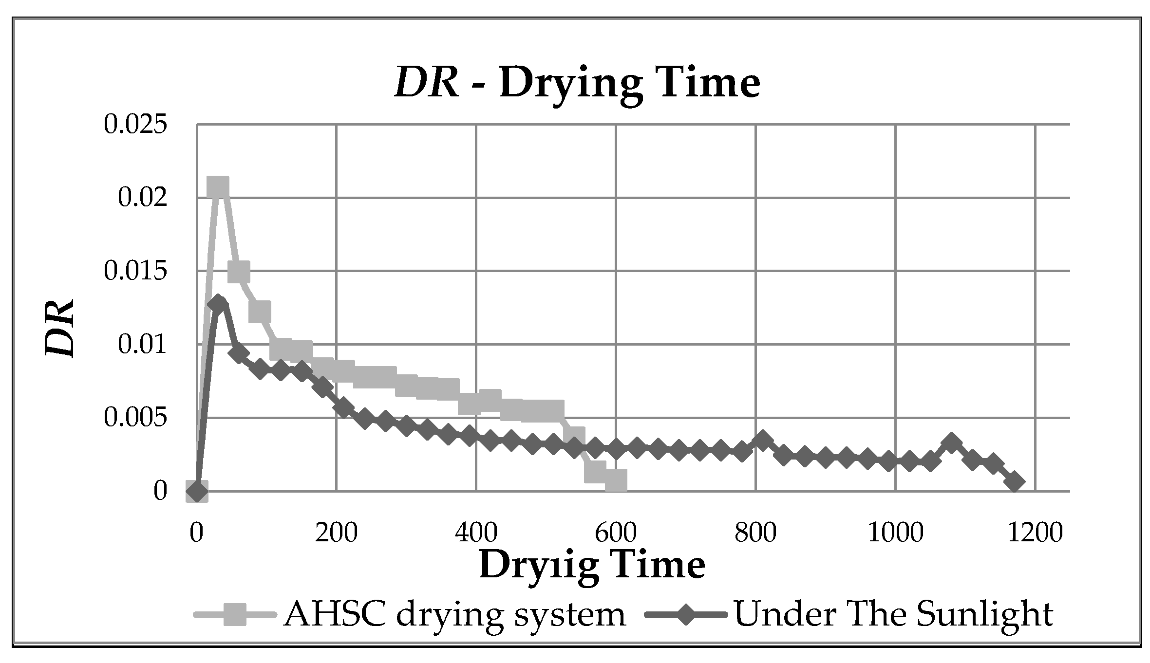
Figure 8.
hc changing with drying time.

Figure 9.
Actual and Predicted data of hc for normalized polynomial kernel.

Figure 10.
Actual and Predicted data of hc for Pearson VII (PUK) kernel.
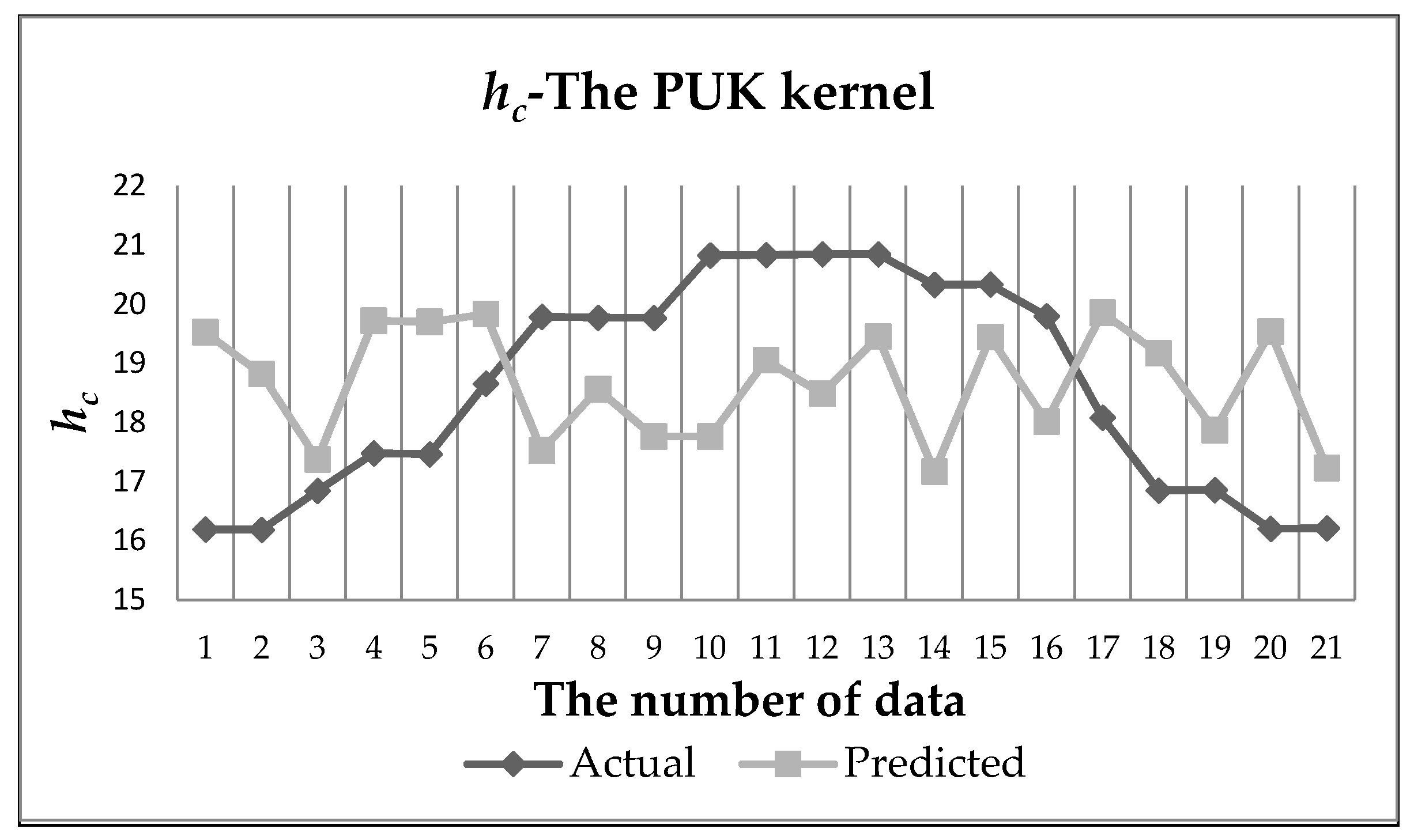
Figure 11.
Actual and Predicted data of hc for radial basis function (RBF) kernel.

Table 1.
Accuracy Criteria and Formulas.
| Accuracy Criteria | Formulas | Parameters |
|---|---|---|
| MAE | P: Predicted Value | |
| A: Actual Value | ||
| n: Total Estimated Value | ||
| RMSE | P: Predicted Value | |
| A: Actual Value | ||
| n: Total Estimated Value | ||
| RAE | P: Predicted Value | |
| A: Actual Value | ||
| A’: Average Of Actual Values | ||
| RRAE | P: Predicted Value | |
| A: Actual Value | ||
| A’: Average Of Actual Values |
Table 2.
The kernel functions and parameters used in support vector machine (SVM).
| Kernel Function | Formulas | Parameters |
|---|---|---|
| The normalized polynomial kernel | d: degree of polynomial | |
| The radial-based function (RBF) kernel | γ: kernel dimension | |
| Pearson VII (PUK) kernel | ω,: Pearson width parameters |
Table 3.
Air heated solar collector (AHSC) drying system experiment data.
| Time (min.) | Panel Inlet Temperature (°C) | Panel Outlet Temperature (°C) | Panel Glass Temperature (°C) | Panel Floor Temperature (°C) | Drying Cabinet Inlet Temp. (°C) | Drying Cabinet Outlet Temperature (°C) | Drying Cabinet Temperature (°C) | Drying Cabinet Moisture (%) | Radiation (W/m²) | Drying Cabinet Air Velocity (m/s) | Product Weight (gram) | Ti (°C) | MCw (%) |
|---|---|---|---|---|---|---|---|---|---|---|---|---|---|
| 0 | 31.3 | 54.9 | 40.7 | 34.0 | 49.1 | 40.8 | 44.0 | 19.6 | 431.7 | 1.2 | 238.4 | 37.7 | 83.1 |
| 30 | 31.9 | 59.0 | 41.2 | 34.5 | 52.5 | 41.5 | 45.3 | 22.6 | 448.6 | 1.2 | 213.3 | 38.6 | 81.1 |
| 60 | 32.7 | 62.3 | 41.8 | 34.8 | 53.4 | 42.1 | 46.8 | 18.5 | 505.5 | 1.3 | 195.2 | 39.8 | 79.3 |
| 90 | 33.3 | 63.4 | 43.0 | 35.2 | 54.3 | 42.9 | 46.5 | 16.6 | 570.5 | 1.4 | 180.4 | 40.1 | 77.6 |
| 120 | 33.8 | 71.0 | 51.8 | 40.4 | 61.1 | 48.2 | 51.9 | 16.2 | 651.2 | 1.4 | 168.7 | 44.8 | 76.1 |
| 150 | 34.5 | 71.8 | 53.3 | 40.8 | 63.6 | 50.6 | 55.0 | 15.9 | 795.9 | 1.6 | 157.2 | 46.2 | 74.3 |
| 180 | 35.6 | 72.9 | 54.0 | 42.7 | 63.3 | 52.2 | 56.7 | 15.5 | 838.6 | 1.8 | 147.1 | 48 | 72.6 |
| 210 | 36.8 | 75.4 | 58.1 | 45.0 | 68.6 | 57.8 | 59.1 | 13.3 | 871.7 | 1.8 | 137.2 | 49.1 | 70.6 |
| 240 | 37.3 | 79.3 | 59.8 | 46.2 | 69.1 | 58.1 | 60.2 | 12.5 | 929.0 | 1.8 | 127.8 | 50.3 | 68.4 |
| 270 | 37.4 | 83.8 | 61.3 | 42.9 | 71.1 | 60.2 | 63.1 | 10.2 | 970.5 | 2.0 | 118.4 | 51.7 | 65.9 |
| 300 | 37.9 | 79.9 | 59.0 | 39.8 | 70.1 | 59.1 | 61.7 | 10.2 | 952.6 | 2.0 | 109.7 | 49.8 | 63.2 |
| 330 | 38.5 | 75.3 | 55.1 | 39.3 | 64.4 | 53.3 | 55.6 | 10.1 | 931.8 | 2.0 | 101.2 | 47.1 | 60.2 |
| 360 | 39.6 | 70.9 | 51.3 | 37.2 | 61.7 | 50.7 | 53.8 | 9.9 | 867.0 | 2.0 | 92.8 | 46.2 | 56.5 |
| 390 | 40.5 | 69.8 | 50.2 | 36.4 | 60.4 | 49.6 | 50.1 | 9.5 | 815.9 | 1.9 | 85.6 | 43.9 | 52.9 |
| 420 | 41.6 | 67.7 | 46.2 | 35.2 | 56.8 | 45.1 | 47.8 | 9.3 | 764.5 | 1.9 | 78.1 | 41.1 | 48.4 |
| 450 | 40.3 | 65.9 | 43.9 | 35.8 | 54.4 | 43.9 | 45.3 | 9.1 | 710.5 | 1.8 | 71.4 | 38.1 | 43.5 |
| 480 | 37.9 | 64.5 | 42.7 | 34.8 | 52.3 | 41.8 | 44.3 | 8.8 | 626.0 | 1.5 | 64.8 | 38 | 37.8 |
| 510 | 34.6 | 59.5 | 41.0 | 34.6 | 50.8 | 38.7 | 42.3 | 8.7 | 526.0 | 1.3 | 58.2 | 35.2 | 30.7 |
| 540 | 31.8 | 52.1 | 40.6 | 34.1 | 47.7 | 37.1 | 41.5 | 8.7 | 518.7 | 1.3 | 53.8 | 34.1 | 25.0 |
| 570 | 30.8 | 51.2 | 40.2 | 34.0 | 45.3 | 36.1 | 40.3 | 8.6 | 457.5 | 1.2 | 52.2 | 33.8 | 22.8 |
| 600 | 30.6 | 50.6 | 39.7 | 33.8 | 43.6 | 35.3 | 37.4 | 8.5 | 436.6 | 1.2 | 51.3 | 33.2 | 21.4 |
Table 4.
Under the sun drying experiment data.
| Time | Outdoor Temp. (°C) | Radiation (W/m²) | Product Weight (Gram) | Air Velocity (m/s) | Moisture (%) | Ti (°C) | MCw (%) |
|---|---|---|---|---|---|---|---|
| 0 | 31.9 | 423.9 | 238.4 | 0.5 | 15.0 | 18.1 | 83.1 |
| 30 | 33.8 | 443.3 | 223.0 | 0.5 | 15.0 | 24.8 | 81.9 |
| 60 | 34.7 | 556.1 | 211.6 | 0.5 | 15.0 | 26.6 | 80.9 |
| 90 | 34.9 | 562.3 | 201.5 | 0.6 | 10.0 | 27.1 | 80.0 |
| 120 | 35.2 | 673.1 | 191.5 | 0.6 | 10.0 | 28.2 | 78.9 |
| 150 | 35.8 | 730.2 | 181.6 | 0.8 | 12.0 | 28.8 | 77.8 |
| 180 | 37.1 | 737.6 | 173.0 | 0.8 | 10.0 | 29.7 | 76.7 |
| 210 | 37.8 | 787.6 | 166.1 | 0.9 | 10.0 | 30.1 | 75.7 |
| 240 | 38.1 | 833.1 | 160.1 | 0.9 | 10.0 | 32.2 | 74.8 |
| 270 | 39.5 | 873.7 | 154.3 | 0.9 | 10.0 | 33.8 | 73.9 |
| 300 | 39.8 | 899.2 | 148.9 | 0.9 | 5.0 | 33.9 | 72.9 |
| 330 | 40.8 | 917.6 | 143.8 | 0.9 | 5.0 | 34.1 | 72.0 |
| 360 | 41.7 | 889.7 | 139.1 | 0.9 | 5.0 | 34.2 | 71.0 |
| 390 | 43.1 | 817.6 | 134.5 | 0.9 | 5.0 | 35.8 | 70.0 |
| 420 | 42.2 | 733.7 | 130.3 | 0.8 | 10.0 | 35.1 | 69.1 |
| 450 | 41.1 | 644.0 | 126.1 | 0.7 | 10.0 | 34.2 | 68.0 |
| 480 | 39.2 | 606.1 | 122.2 | 0.6 | 10.0 | 33.1 | 67.0 |
| 510 | 36.6 | 546.0 | 118.3 | 0.6 | 10.0 | 31.8 | 65.9 |
| 540 | 34.6 | 516.1 | 114.7 | 0.6 | 10.0 | 29.4 | 64.8 |
| 570 | 34.2 | 486.1 | 111.1 | 0.5 | 10.0 | 27.4 | 63.7 |
| 600 | 33.8 | 356.2 | 107.6 | 0.5 | 10.0 | 25.2 | 62.5 |
| 630 | 31.2 | 434.48 | 104 | 0.5 | 15 | 23.3 | 61.2 |
| 660 | 32.8 | 473.05 | 100.5 | 0.5 | 15 | 24.1 | 59.9 |
| 690 | 33.3 | 509.06 | 97.1 | 0.5 | 15 | 24.8 | 58.5 |
| 720 | 34.8 | 554.08 | 93.7 | 0.6 | 10 | 25.5 | 57.0 |
| 750 | 35.1 | 657.23 | 90.3 | 0.6 | 10 | 26.6 | 55.3 |
| 780 | 35.2 | 674.15 | 87 | 0.7 | 12 | 27.4 | 53.7 |
| 810 | 35.2 | 698.6 | 82.8 | 0.8 | 10 | 27.5 | 51.3 |
| 840 | 35.2 | 780.44 | 79.8 | 0.9 | 10 | 27.5 | 49.5 |
| 870 | 35.4 | 810.4 | 76.9 | 0.9 | 10 | 27.8 | 47.6 |
| 900 | 35.5 | 874.7 | 74.1 | 0.9 | 10 | 28 | 45.6 |
| 930 | 37.8 | 907.68 | 71.3 | 0.9 | 5 | 30.1 | 43.4 |
| 960 | 38.3 | 922.42 | 68.6 | 0.9 | 5 | 32.6 | 41.2 |
| 990 | 38.8 | 883.15 | 66.1 | 0.9 | 5 | 32.9 | 39.0 |
| 1020 | 39.2 | 734.71 | 63.6 | 0.9 | 5 | 33.8 | 36.6 |
| 1050 | 38.8 | 645.67 | 61.1 | 0.8 | 10 | 33 | 34.0 |
| 1080 | 39.3 | 612.3 | 57.1 | 0.7 | 10 | 33.7 | 29.4 |
| 1110 | 39.6 | 528.31 | 54.5 | 0.6 | 10 | 34.1 | 26.0 |
| 1140 | 38.2 | 483.71 | 52.2 | 0.6 | 10 | 33.4 | 22.8 |
| 1170 | 36.5 | 480.09 | 51.4 | 0.6 | 10 | 30.2 | 21.4 |
Table 5.
Error rates for SVM regression.
| Kernel Models | MAE | RMSE | RAE | RRAE |
|---|---|---|---|---|
| The normalized polynomial kernel | 0.279 | 0.3351 | 16.464% | 18.304% |
| The Pearson VII function-based universal (PUK) kernel | 0.4013 | 0.5175 | 23.682% | 28.265% |
| The radial-based function (RBF) kernel | 0.7048 | 0.84 | 41.593% | 45.877% |
Table 6.
Support vectors obtained in SVM regression for hc.
| The normalized polynomial kernel | hc = 0.3416 − 0.1255 × k[0] − 1.0 × k[1] +0.5860 × k[2] +1.0 × k[3] − 1.0 × k[4] − 1.0 × k[5] +1.0 × k[6] − 0.2071 × k[7] − 1.0 × k[8] +1.0 × k[9] +1.0 × k[10] +1.0 × k[11] − 0.3152 × k[12] − 1.0 × k[13] +1.0 × k[14] +0.4007 × k[15] − 1.0 × k[16] − 0.7025 × k[17] +1.0 × k[18] − 0.7020 × k[19] +0.06567 × k[20] |
| The Pearson VII function-based universal (PUK) kernel | hc = 0.4527 − 0.3017 × k[0] − 0.2619 × k[1] − 0.08917 × k[2] +0.03710 × k[3]− 0.24516 × k[4] − 0.05424 × k[5] +0.2599 × k[6] +0.0062 × k[7] − 0.0103 × k[8] +0.3469 × k[9] +0.1565 × k[10] +0.1490 × k[11] +0.3641 × k[12] − 0.1278 × k[13] +0.2997 × k[14] +0.1389 × k[15] − 0.0721 × k[16] − 0.2559 × k[17] +0.2316 × k[18] − 0.4044 × k[19] − 0.16728 × k[20] |
| The radial-based function (RBF) kernel | hc = 0.384 − 1.0 × k[0] − 1.0 × k[1] − 1.0 × k[2] − 0.2996 × k[3] − 1.0 × k[4] − 1.0 × k[5] +1.0 × k[6] +1.0 × k[7] +0.0764 × k[8] +1.0 × k[9] +1.0 × k[10] +1.0 × k[11] +1.0 × k[12] +1.0 × k[13] +1.0 × k[14] +1.0 × k[15] +0.2232 × k[16] − 1.0 × k[17] − 1.0 × k[18] − 1.0 × k[19] − 1.0 × k[20] |
© 2018 by the authors. Licensee MDPI, Basel, Switzerland. This article is an open access article distributed under the terms and conditions of the Creative Commons Attribution (CC BY) license (http://creativecommons.org/licenses/by/4.0/).
Share and Cite
MDPI and ACS Style
Das, M.; Akpinar, E.K. Investigation of Pear Drying Performance by Different Methods and Regression of Convective Heat Transfer Coefficient with Support Vector Machine. Appl. Sci. 2018, 8, 215. https://doi.org/10.3390/app8020215
AMA Style
Das M, Akpinar EK. Investigation of Pear Drying Performance by Different Methods and Regression of Convective Heat Transfer Coefficient with Support Vector Machine. Applied Sciences. 2018; 8(2):215. https://doi.org/10.3390/app8020215
Chicago/Turabian StyleDas, Mehmet, and Ebru Kavak Akpinar. 2018. "Investigation of Pear Drying Performance by Different Methods and Regression of Convective Heat Transfer Coefficient with Support Vector Machine" Applied Sciences 8, no. 2: 215. https://doi.org/10.3390/app8020215
Note that from the first issue of 2016, this journal uses article numbers instead of page numbers. See further details here.