Virtual Source Array-Based Multiple Time-Reversal Focusing

1
Department of Convergence Study on the Ocean Science and Technology, Korea Maritime and Ocean University, Busan 606-791, Korea
2
Scripps Institution of Oceanography, La Jolla, CA 92093-0238, USA
*
Author to whom correspondence should be addressed.
Appl. Sci. 2018, 8(1), 99; https://doi.org/10.3390/app8010099
Submission received: 20 November 2017
/
Revised: 3 January 2018
/
Accepted: 9 January 2018
/
Published: 11 January 2018
(This article belongs to the Special Issue Underwater Acoustics, Communications and Information Processing)
Abstract
:Time reversal (TR) is the process of generating a spatio-temporal focus at a probe source (PS) location by transmitting a time-reversed version of a received signal. While TR focusing requires the PS for a coherent acoustic focus at its origin, the requirement of the PS has been partially relaxed by the introduction of the concept of a virtual source array (VSA) (J. Acoust. Soc. Am. 2009, 125, 3828–3834). A VSA can serve as a remote platform or lens and redirect a focused field to a selected location beyond the VSA for which the field is assumed as a homogeneous medium with constant sound speed. The objective of this study is to extend VSA-based single TR focusing to simultaneous multiple focusing. This is achieved using the optimization theory by employing the multiple constraints method derived from a constraint matrix, which consists of appropriately synchronized transfer functions. Through numerical simulations, it is found that simultaneous multiple focusing can be achieved with distortionless response at selected multiple locations, and its performance degrades in the presence of sound speed mismatch. For achieving robust multiple focusing in the mismatch environment, singular value decomposition is applied to obtain the weight vector (i.e., backpropagation vector) that best approximates the column vectors of the constraint matrix. Numerical simulation results show that VSA-based multiple TR focusing using SVD is not a method to simultaneously focus on multiple locations, but a method of constructing a field which robustly passes through multiple locations in sound speed mismatch environment.
1. Introduction
Over the last several decades, time reversal (TR) processing has been extensively studied in various fields [1,2,3]. In TR processing, a transmitted probe signal is received at an array of source-receive elements, which is referred to as a time-reversal mirror (TRM), and the received signal is time reversed to be backpropagated into the medium. If the propagation medium is static, TR processing results in coherent acoustic focusing (or pulse compression) at the probe source (PS) location where the signal was generated. One of the main advantages of TR processing is generating a focused field without a-priori knowledge about the propagation medium (i.e., self-adaptive) because of the TR invariance of the wave equation.
The adaptive time-reversal mirror (ATRM), proposed by Kim et al. [4], backpropagates the weight vector obtained as the optimal solution of an objective function with a single imposed constraint. It can focus distortionless response at a single location while simultaneously forming nulls by minimizing the total reception power at different arbitrary locations. The ATRM can be applied directly to selective focusing on a weak target [4] and to underwater multiuser communications to mitigate cross talk [5]. By extension, multiple TR focusing based on adaptive methods was proposed for the long range underwater communication [6] and stable focusing in a fluctuating ocean environment [7].
However, a practical limitation of TR processing is the requirement of a PS to obtain a spatio-temporal focus at the PS location; this is the primary weakness of TR processing. Virtual source array (VSA)-based TR focusing, which was proposed by Walker et al. [8], was designed to perform TR focusing without the requirement of a PS and provide a resolution comparable to that of conventional TR focusing. The basic idea is that a-priori sampled (or measured) transfer functions between the TRM and VSA are appropriately time delayed prior to backpropagation from the TRM. These functions are referred to as synchronized transfer functions. Consequently, the backpropagated field is steered over the VSA to a selected location for which the transfer function is unknown.
The objective of this study is to extend the VSA-based single TR focusing to simultaneous multiple focusing at arbitrarily selected locations. To achieve this, the multiple constraints method (MCM) [9] is applied by imposing a set of constraints in the formulation of the weight vector (i.e., backpropagation vector). Then, the detailed response of VSA-based multiple TR focusing to sound speed mismatch is examined. Further, singular value decomposition (SVD) [7,10] is applied to achieve robust VSA-based multiple TR focusing in the sound speed mismatch environment. It was found that a wavefield is created to pass through multiple locations, but not necessarily at the same time. As multiple TR focusing without the VSA is applicable only when two-way propagation is involved (i.e., at least one physical PS is needed), which extends its applicability to underwater communications or focal-spot broadening to achieve stable focusing, our approach can be more attractive in these practical applications because one-way propagation can only be used in implementing multiple focusing at arbitrarily selected locations beyond the VSA, if a-priori measured transfer functions between the TRM and VSA are updated at regular intervals, e.g., a week [3].
The remainder of the paper is organized as follows. Section 2 reviews VSA-based single TR focusing. In Section 3, the approach is extended to simultaneous multiple focusing using the adaptive method, where the backpropagation vector is obtained with multiple constraints. In Section 4, the performance of VSA-based multiple TR focusing is compared based on two different profiles (isovelocity and downward-refracting) via numerical simulations in an ocean waveguide. The robustness of the method is investigated in the presence of sound speed mismatch in Section 5, followed by a summary in Section 6.
2. Review of VSA-Based TR Focusing
The details of the applications of the VSA concept in TR focusing can be found in Refs. [8,11,12]. This section summarizes VSA-based single TR focusing. The phase-conjugated (or time-reversed) field at a field location, , in a frequency domain can be written as
where denotes the field from the mth element of the TRM to an arbitrary field location, , and and denote the complex conjugate and Hermitian transpose, respectively. In vector notation, and are specified as column vectors. The field for backpropagation, denoted by , provides the following synchronized transfer function:
where represents a-priori sampled transfer functions between the TRM and VSA. Prior to backpropagation, the time delay, , of the line of sight between the nth element of the VSA and the selected location, , is applied to the sampled transfer functions assuming that the field beyond the VSA is a homogeneous medium with constant sound speed, c.
3. Adaptive VSA-Based Multiple TR Focusing
In this section, VSA-based single TR focusing is extended to simultaneous multiple focusing at arbitrarily selected locations beyond the VSA (hereafter referred to as the adaptive VSA). Generally, the weight vector, , can be derived from the following objective function with multiple constraints:
The solution to this optimization problem is well known and can be found using the Lagrange multiplication method as
where is the cross spectral density matrix, which contains the information of the synchronized transfer functions corresponding to the selected multiple locations.
For simplicity, we consider only two focal locations, and , which can be easily generalized to more locations. and denote a small diagonal loading factor for inverse matrix calculation and the identity matrix, respectively. The constraint response, , which is frequently referred to as the directional constraint [13], is a matrix that forces the response of multiple locations to be unity. represents an constraint matrix, which is composed of synchronized transfer functions for the selected locations.
In conventional multiple TR focusing [6], this approach might be impractical because the transfer functions corresponding to the different PS locations are required to form the constraint matrix, ; this requires additional measurements. However, our approach simply applies the time delay corresponding to the selected multiple locations to a-priori sampled transfer functions (i.e., synchronized transfer functions). Thus, the constraint matrix, , can be easily formed when the sampled transfer functions are provided. By backpropagating the weight vector, , with multiple constraints, simultaneous multiple focusing with distortionless response, , can be achieved at the selected locations beyond the VSA,
where the weight vector, , reduces to in VSA-based single TR focusing.
4. Simulations in Waveguide
In this section, we investigate the behavior of the adaptive VSA using numerical simulations. As the weight vector, , is derived from the constraint matrix, , which partially includes the characteristic of the homogeneous medium with constant sound speed, c, the performance of the adaptive VSA might be sensitive if the actual sound speed in the water column is different from the assumed constant sound speed, c. Thus, a fundamental question is whether adaptivity (i.e., MCM) can be applied to VSA-based TR focusing.
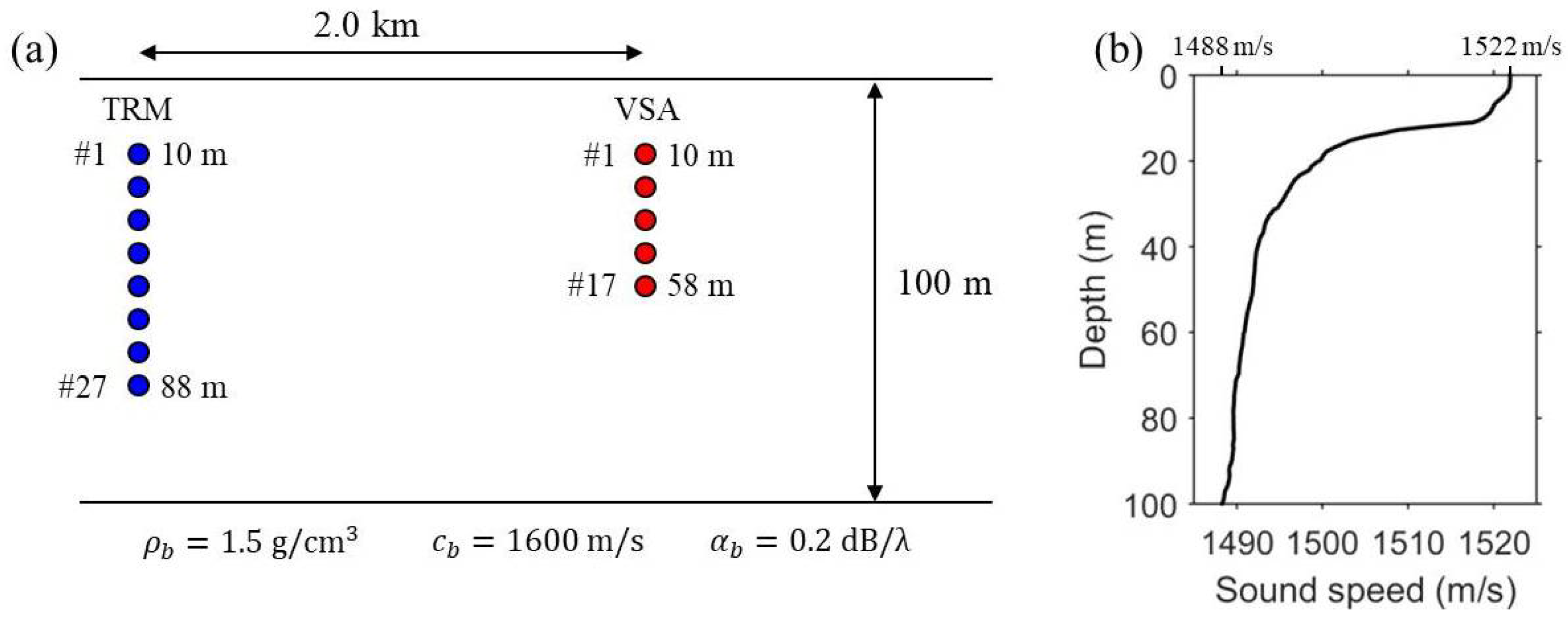
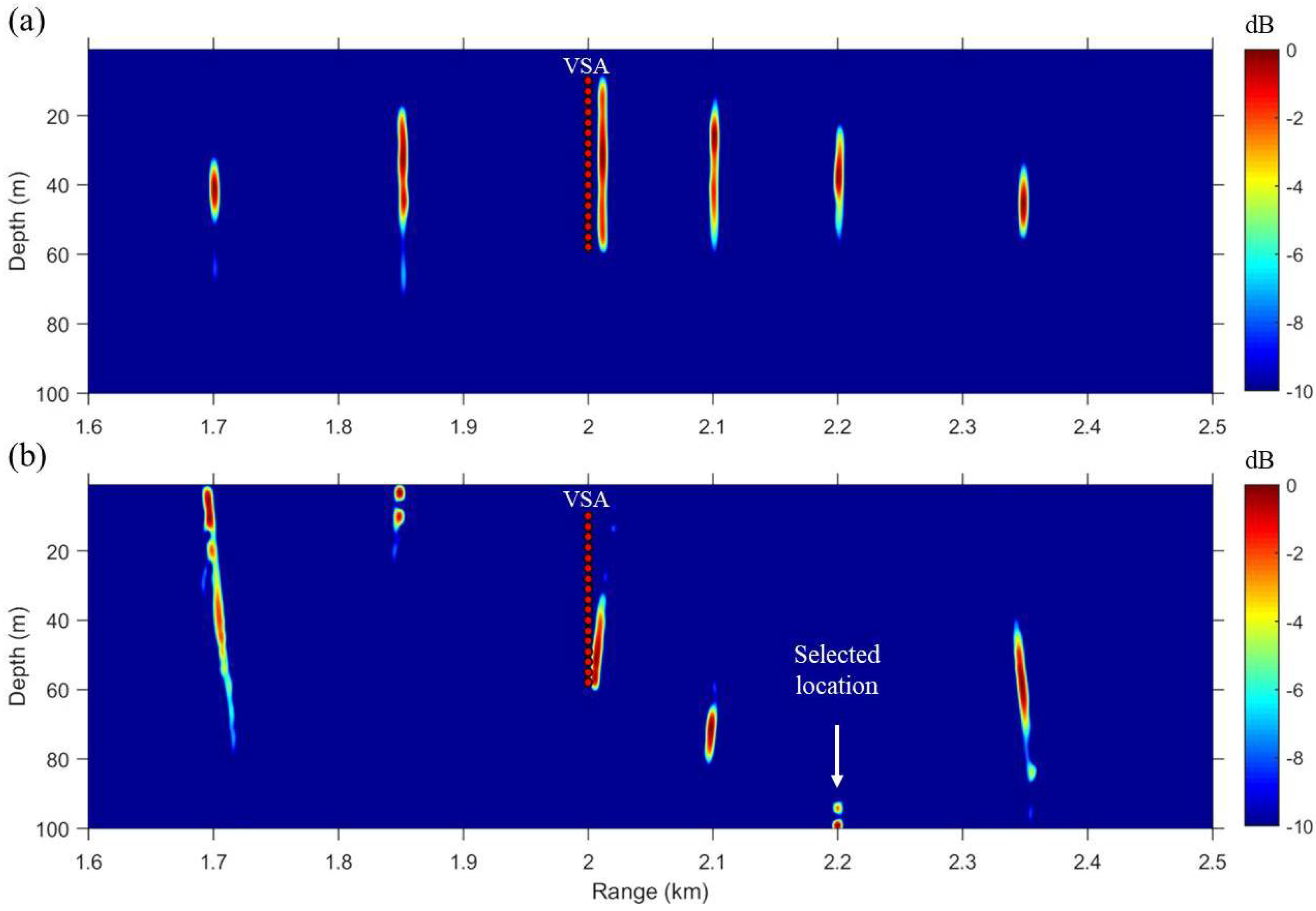
The schematic of the numerical simulations is illustrated in Figure 1. The TRM consists of 27 elements spanning a 78-m aperture with a 3-m element spacing in 100-m deep shallow water. Similarly, the VSA is a 48-m long 17-element vertical array with a 3-m element spacing, located 2 km from the TRM. A normal mode propagation model [14] is used for numerical simulations with the following geoacoustic parameters of the sea floor: density g/cm, compressional sound speed m/s, and attenuation dB/. A range-independent environment with a simple half-space bottom and a downward-refracting sound speed profile (SSP) shown in Figure 1b is assumed. An average sound speed of c = 1500 m/s across the VSA is used for the line-of-sight time delay, . Figure 2 presents the simulated backpropagation results of VSA-based single TR focusing in the ocean waveguide shown in Figure 1. Each of the backpropagated fields is normalized with respect to its own maximum and superimposed with the corresponding snapshot times. A 10-ms pulse with a center frequency of 500 Hz and a Hann window is used for probe transmission. It is clear that the backpropagated synchronized field is steered over the VSA to a selected location (r = 2.2 km, z = 100 m) (see Figure 2b) compared to when no time delay is applied (see Figure 2a).
4.1. Superposition Method
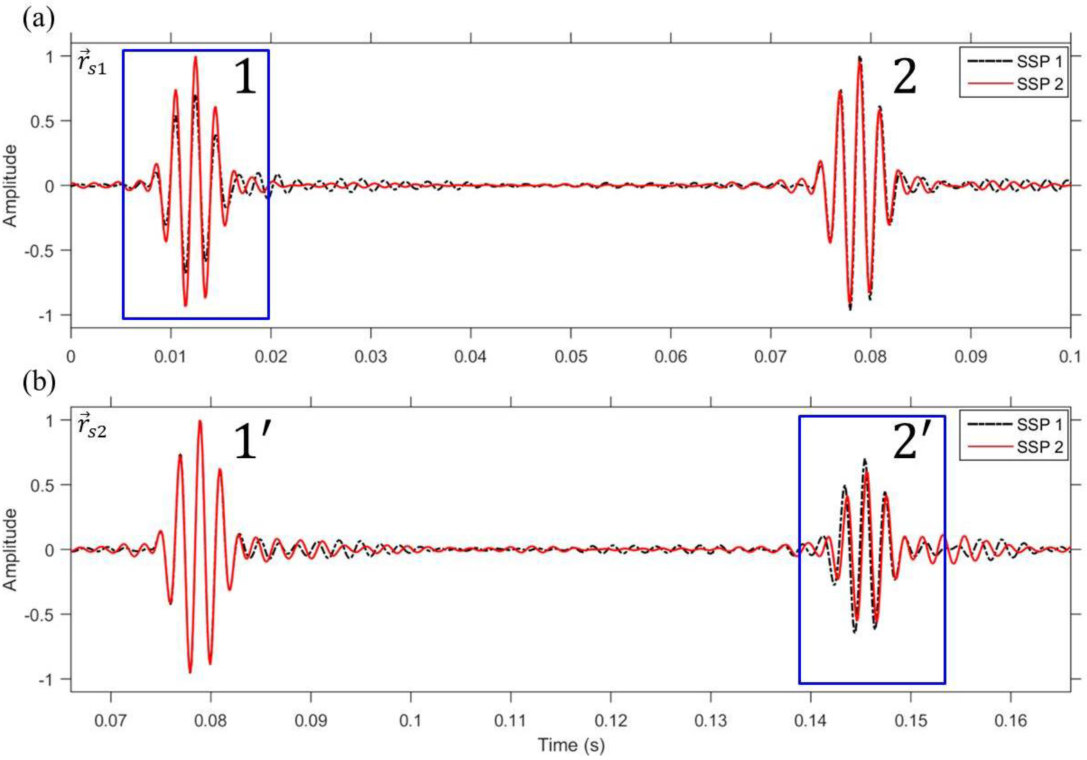
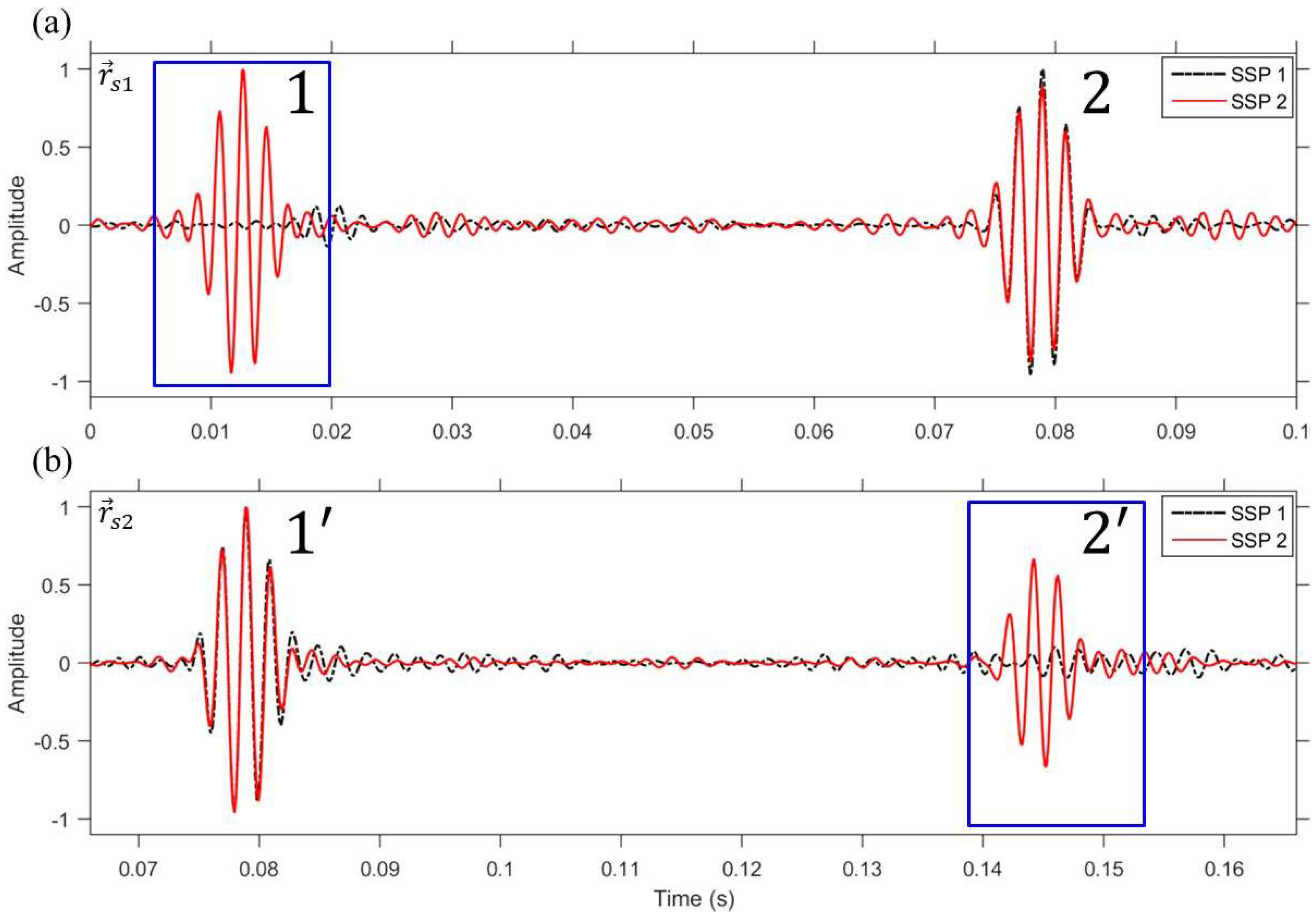
First, we take a look at the case of the superposition method which is the most intuitive method of simultaneous multiple focusing. The sampled transfer functions between the TRM and VSA are time delayed corresponding to a line-of-sight distance between the VSA and selected locations = (2.2 km, 50 m) and = (2.3 km, 50 m), respectively, and then superimposed prior to backpropagation from the TRM. Figure 3 shows the simulated time series at two selected locations for two different profiles, i.e., the isovelocity with a sound speed of c = 1500 m/s (SSP 1, dot-dashed) and the downward-refracting SSP (SSP 2, solid). Since the sampling frequency is 7500 Hz and fast Fourier transform size is 8192, the time duration is 1.09 s long. This time duration is not sufficient to prevent aliasing on the time axis as the pulse propagates (e.g., ≈ 1.5 s). Thus, a random time shift was applied to the time series results. Not surprisingly, imperfect pulse compression is achieved at both selected locations, (see Figure 3a) and (see Figure 3b), owing to the residual term of the phase-conjugated field,
where the residual term can be presented as in the case of the phase-conjugated field at location .
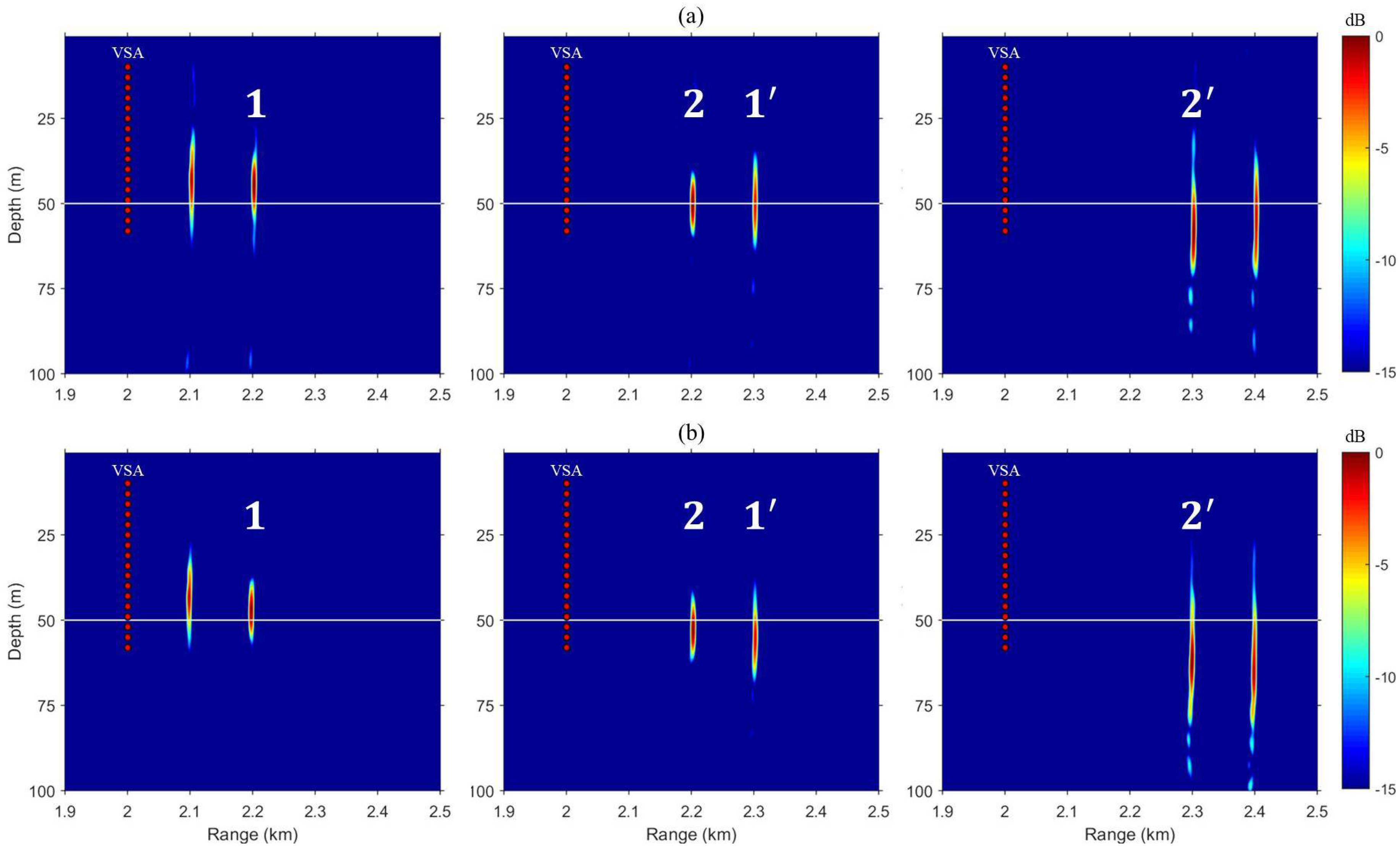
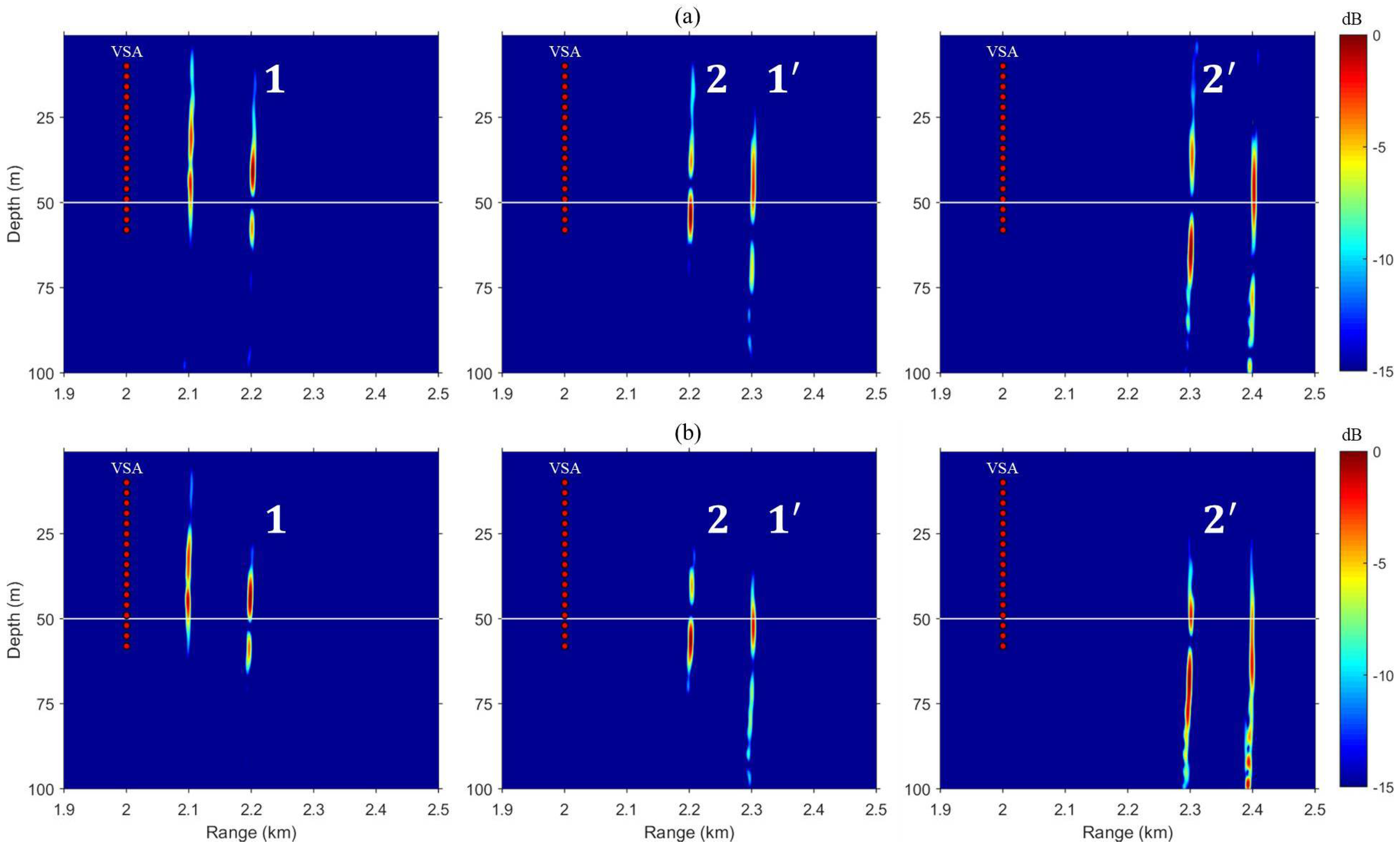
Figure 4 shows snapshot results of field propagation when the superimposed vector is backpropagated from the TRM, and each number corresponds to a time series at multiple locations in Figure 3. Panels (a) and (b) in Figure 4 represent the case of isovelocity SSP and downward-refracting SSP, respectively. As the synchronized transfer functions corresponding to the two locations are superimposed and backpropagated, it can be seen that two fields with the appropriate distance are propagated for simultaneous multiple focusing. Thus, the residual term occurs as fields 1 (left) and (right) pass through multiple locations. Also, as shown in the lower panel, the focused fields (i.e., 2 and ) are slightly shifted down by the sound speed structure, but are still included in the focal resolution. The solid line indicates the depth of the focal location (i.e., 50 m).
4.2. Adaptive VSA
Figure 5 shows the simulation result of the adaptive VSA. To emphasize the relationship between sound speed mismatch and the performance changes in multiple focusing, the time series at the selected locations are normalized with respect to its own maximum as well as the existence of noise is not considered in numerical simulations. The weight vector, , is obtained from Equation (4); then, it is time reversed and backpropagated. Panels (a) and (b) in Figure 5 show the simulated time series at the selected locations. A comparison between the two different profiles (dot-dashed and solid) provides strong evidence that the adaptive VSA with multiple constraints is sensitive to sound speed mismatch (solid) because the residual signal, denoted by a rectangular box, is still observable compared to the isovelocity case (dot-dashed).
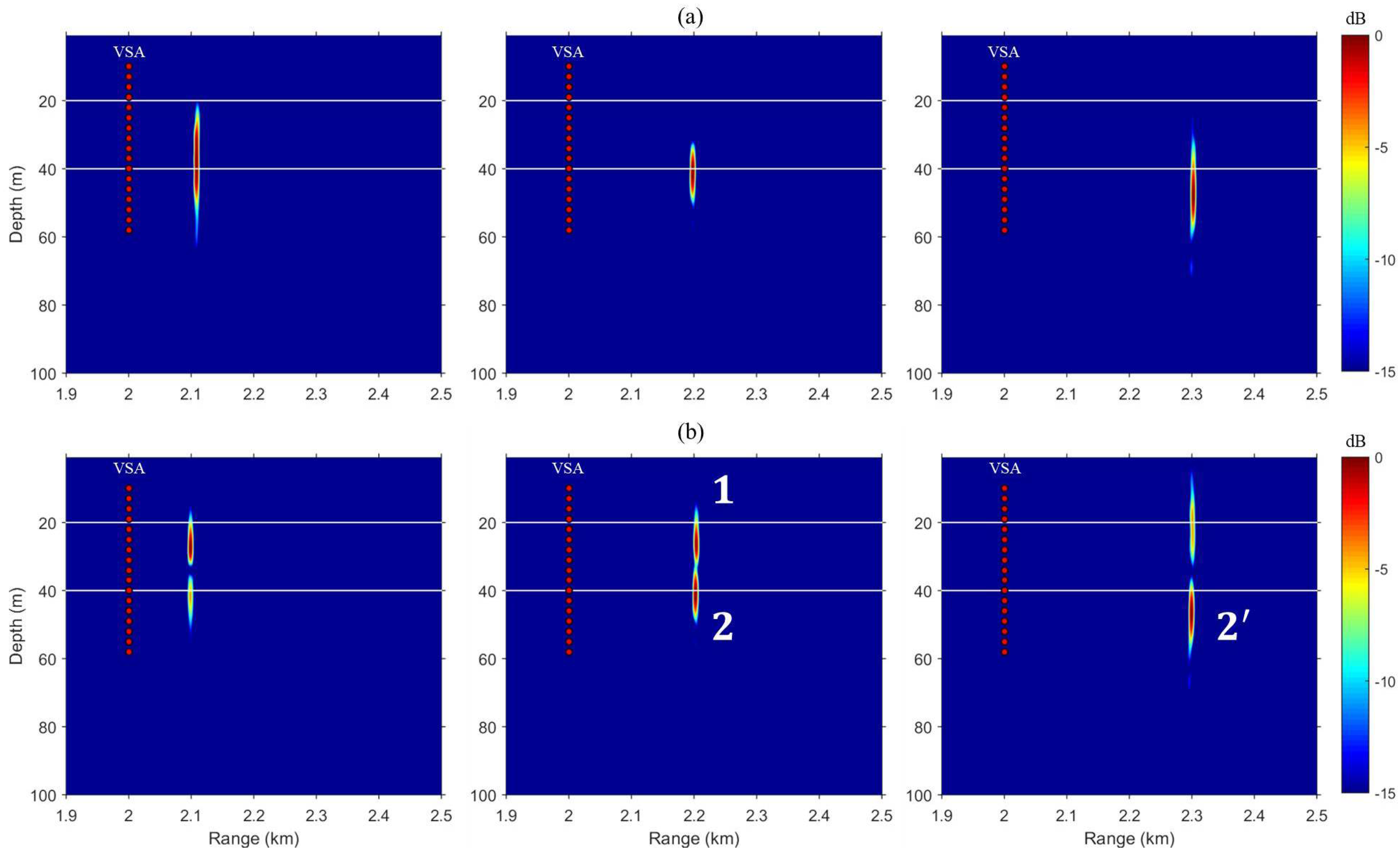
In fact, the weight vector, , with multiple constraints, , can be expressed as the sum of and with constraints and , respectively. Thus, the weight vector, , can focus distortionless response at the selected locations while simultaneously placing the null at different locations, as shown in Figure 6, providing time series as a function of depth at range of 2.3 km, which corresponds to Figure 5b. For isovelocity (see Figure 6a), it is clear that the residual signal is mitigated as seen in the inset at the bottom right, which is magnified to highlight the location where the null is to be placed. However, imperfect pulse compression is achieved when the actual SSP in the water column is different from the assumed sound speed, c, beyond the VSA owing to the failure of null placement (i.e., sound speed mismatch) (see Figure 6b).
Figure 7 provides more insight into how nulls are placed in multiple locations through field propagation. Interestingly, in the case of the isovelocity SSP (see Figure 7a), nulls are placed at the corresponding locations, and (i.e., 1 and ) as the field is propagated. However, in the case of the downward-refracting SSP (see Figure 7b), it is clearly shown the nulls are placed at different locations due to the sound speed mismatch.
5. Robust VSA-Based Multiple TR Focusing
The approach described in this section partially retains Krolik’s application [10] of SVD to matched-field processing (MFP) and the stability of TR focusing in a fluctuating ocean environment [7]. However, it extends to VSA-based multiple TR focusing, rather than MFP or conventional TR focusing. As investigated in Section 4.2, the performance of the adaptive VSA is significantly degraded in the presence of sound speed mismatch owing to the fact that the constraint matrix, , partially contains the characteristic of the homogeneous field with constant sound speed, c. In practice, the constraint matrix, , can be decomposed into several component matrices using SVD with a best rank K approximation,
where is an matrix whose columns are left singular vectors, is a matrix whose off-diagonal entries are zeros and diagonal elements are the singular values of , and is a matrix whose columns are right singular vectors. Indeed, the first singular vector corresponding to the largest singular value is sufficient to approximate the columns of constraint matrix, ; thus, the backpropagation vector, , is reformulated with the response vector, ,
Figure 8 and Figure 9 provide a clear understanding of VSA-based multiple TR focusing using SVD method in sound speed mismatch environment. The selected locations were changed to = (2.2 km, 20 m) and = (2.3 km, 40 m) to show the dramatic results of VSA-based multiple TR focusing using SVD method, and the results were compared to VSA-based single TR focusing results at a selected location, = (2.3 km, 40 m).
In the case of VSA-based single TR focusing (dot-dashed), pulse compression is achieved at the selected location, = (2.3 km, 40 m), as expected (see Figure 8b), but because the field is not propagated to the location, = (2.2 km, 20 m) (see Figure 9a), incomplete pulse compression and signal spread over time are observed (see Figure 8a). Note that the normalization of the axis amplified low-amplitude noise (dot-dashed in Figure 8a). On the other hand, using the SVD method, pulse compression is fully achieved at both selected locations, and , as shown in Figure 8 (solid), which provides robustness to sound speed mismatch environment. In addition, Figure 9 shows how the SVD-based method, unlike the single focusing, can achieve multiple focusing. Figure 9b shows the snapshot result of the propagated field as the weight vector calculated through Equation (9) is back propagated. In this case, the weight vector, , that is backpropagated is a vector that best approximates the synchronized transfer functions corresponding to the two locations, = (2.2 km, 20 m) and = (2.3 km, 40 m), so that one dominant field propagates unlike the MCM-based method. That is, although the SVD-based TR focusing is not a simultaneous focusing method, it is a robust multiple focusing method of forming a field that passes through multiple focal locations even in sound speed mismatch environment. In this case, two fields separated in the vertical direction are propagated to satisfy multiple focusing. The field corresponding to the number 2 is an unnecessary field at the focal location, = (2.2 km, 20 m), but is a field for focusing at the location, = (2.3 km, 40 m) (i.e., the number ).
6. Summary
VSA-based single TR focusing successfully steers the synchronized field to a selected location beyond the VSA for which the field is assumed as a homogeneous medium with constant sound speed. In this study, the approach was extended to simultaneous multiple focusing using the adaptive method (MCM), resulting in pulse compression with mitigation of interference for the isovelocity with the same sound speed as that of the field beyond the VSA. However, in the presence of sound speed mismatch, imperfect pulse compression is achieved because of the failure of placing the null at the desired location owing to the mismatch. To achieve robustness, the constraint matrix is decomposed using SVD to obtain the backpropagation vector that best approximates the column vectors of the constraint matrix. Numerical simulations demonstrate the feasibility of VSA-based multiple TR focusing and validate its robustness.
Acknowledgments
G.B. and J.S.K. were supported by a part of the project titled ‘Development of Ocean Acoustic Echo Sounders and Hydro-Physical Properties Monitoring Systems’, funded by the ministry of Oceans and Fisheries, Korea (20130056).
Author Contributions
G.B. and J.S.K. developed the idea of VSA-based multiple TR focusing. G.B. and H.C.S. had intensive discussions in the numerical simulation results. All of the authors drew conclusions.
Conflicts of Interest
The authors declare no conflict of interest.
Abbreviations
The following abbreviations are used in this manuscript:
| TR | Time reversal |
| TRM | Time-reversal mirror |
| VSA | Virtual source array |
| MCM | Multiple constraints method |
| SVD | Singular value decomposition |
| ATRM | Adaptive time-reversal mirror |
| MFP | Matched-field processing |
| SSP | Sound speed profile |
| PS | Probe source |
References
- Fink, M. Time reversed acoustics. Phys. Today 1997, 50, 34–40. [Google Scholar] [CrossRef]
- Kuperman, W.A.; Hodgkiss, W.S.; Song, H.C.; Akal, T.; Ferla, C.; Jackson, D.R. Phase conjugation in the ocean: Experimental demonstration of an acoustic time reversal mirror. J. Acoust. Soc. Am. 1998, 103, 25–40. [Google Scholar] [CrossRef]
- Hodgkiss, W.S.; Song, H.C.; Kuperman, W.A.; Akal, T.; Ferla, C.; Jackson, D.R. A long-range and variable focus phase-conjugation experiment in shallow water. J. Acoust. Soc. Am. 1999, 105, 1597–1604. [Google Scholar] [CrossRef]
- Kim, J.S.; Song, H.C.; Kuperman, W.A. Adaptive time-reversal mirror. J. Acoust. Soc. Am. 2001, 109, 1817–1825. [Google Scholar]
- Song, H.C.; Kim, J.S.; Hodgkiss, W.S.; Joo, J.H. Crosstalk mitigation using adaptive time reversal. J. Acoust. Soc. Am. 2010, 127, EL19–EL22. [Google Scholar] [CrossRef] [PubMed]
- Kim, J.S.; Shin, K.C. Multiple focusing with adaptive time-reversal mirror. J. Acoust. Soc. Am. 2004, 115, 600–606. [Google Scholar] [CrossRef] [PubMed]
- Kim, S.; Kuperman, W.A.; Hodgkiss, W.S.; Song, H.C.; Edelmann, G.F.; Akal, T. Robust time reversal focusing in the ocean. J. Acoust. Soc. Am. 2003, 114, 145–157. [Google Scholar] [CrossRef] [PubMed]
- Walker, S.C.; Roux, P.; Kuperman, W.A. Synchronized time-reversal focusing with application to imaging from a distant virtual source array. J. Acoust. Soc. Am. 2009, 125, 3828–3834. [Google Scholar] [CrossRef] [PubMed]
- Schmidt, H.; Baggeroer, A.B.; Kuperman, W.A.; Scheer, E.K. Environmentally tolerant beamforming for high-resolution matched field processing: Deterministic mismatch. J. Acoust. Soc. Am. 1990, 88, 1851–1862. [Google Scholar] [CrossRef]
- Krolik, J.L. Matched-field minimum variance beamforming in a random ocean channel. J. Acoust. Soc. Am. 1992, 92, 1408–1419. [Google Scholar] [CrossRef]
- Yu, Z.; Zhao, H.; Gong, X.; Chapman, R. Time-Reversal Mirror-Virtual Source Array Method for Acoustic Imaging of Proud and Buried Targets. IEEE J. Ocean. Eng. 2016, 41, 382–394. [Google Scholar]
- Byun, G.; Kim, J.S. Robust variable range focusing with a virtual source array using the waveguide invariant in underwater. J. Acoust. Soc. Korean 2017, 36, 23–29. (In Korean) [Google Scholar] [CrossRef]
- Takao, K.; Fujita, H.; Nishi, T. An adaptive arrays under directional constraint. IEEE Trans. Antennas Propag. 1976, 24, 662–669. [Google Scholar] [CrossRef]
- Porter, M.B. The Acoustic Toolbox. Available online: http://oalib.hlsresearch.com/Modes/AcousticsToolbox/ (accessed on 25 October 2017).
Figure 1.
(Color online) Schematic of virtual source array (VSA)-based time reversal (TR) focusing and waveguide conditions used for numerical simulations. (a) Different vertical arrays, denoted by time-reversal mirror (TRM) (blue circle) and VSA (red circle), of 27 and 17 elements with 3-m array spacing are considered in 100-m deep shallow water; (b) Sound speed profile used for normal mode simulations.

Figure 2.
(Color online) Simulated VSA-based single TR focusing. Six snapshots of the backpropagated field from the TRM are superimposed with the corresponding snapshot times. Each snapshot is normalized with respect to its own maximum. (a) Without time delay (i.e., ) for a-priori sampled transfer functions; (b) Sampled transfer functions are appropriately time delayed; thus, it is clear that the synchronized field is steered over the VSA to a selected location.

Figure 3.
(Color online) Simulated VSA-based multiple TR focusing using superposition method. The simulated time series are normalized with respect to its own maximum. (a) Time series at = (2.2 km, 50 m); (b) Time series at = (2.3 km, 50 m). The residual signal (denoted by a rectangular box) is clearly observed for the cases of isovelocity with a sound speed of c = 1500 m/s (SSP 1, dot-dashed) and downward-refracting SSP (SSP 2, solid).

Figure 4.
(Color online) Simulated VSA-based multiple TR focusing using superposition method. Each panel represents a backpropagated field corresponding to a different single snapshot time. (a) For isovelocity SSP; (b) For downward-refracting SSP. The numbers here correspond one-to-one with the time series in Figure 3.

Figure 5.
(Color online) Simulated adaptive VSA-based multiple TR focusing for different types of profiles. (a) Time series at = (2.2 km, 50 m); (b) Time series at = (2.3 km, 50 m). While pulse compression is fully achieved for the isovelocity with a sound speed of c = 1500 m/s (SSP 1, dot-dashed), the residual signal (denoted by a rectangular box) is still observable for the downward-refracting SSP (SSP 2, solid).

Figure 6.
(Color online) Time series as a function of depth at a range of 2.3 km, which corresponds to Figure 5b. (a) For isovelocity SSP; (b) For downward-refracting SSP. The null location, denoted by a rectangular box, is magnified and the residual signal is highlighted at the bottom right.
Figure 6.
(Color online) Time series as a function of depth at a range of 2.3 km, which corresponds to Figure 5b. (a) For isovelocity SSP; (b) For downward-refracting SSP. The null location, denoted by a rectangular box, is magnified and the residual signal is highlighted at the bottom right.
Figure 7.
(Color online) Simulated adaptive VSA-based multiple TR focusing using MCM method. Each panel represents a backpropagated field corresponding to a different single snapshot time. (a) For isovelocity SSP; (b) For downward-refracting SSP. The numbers here correspond one-to-one with the time series in Figure 5.

Figure 8.
(Color online) Comparison of the simulated time series for the weight vector, , with VSA-based single TR focusing (dot-dashed) and VSA-based multiple TR focusing using singular value decomposition (SVD) (solid) in sound speed mismatch environment. (a) Time series at = (2.2 km, 20 m); (b) Time series at = (2.3 km, 40 m).
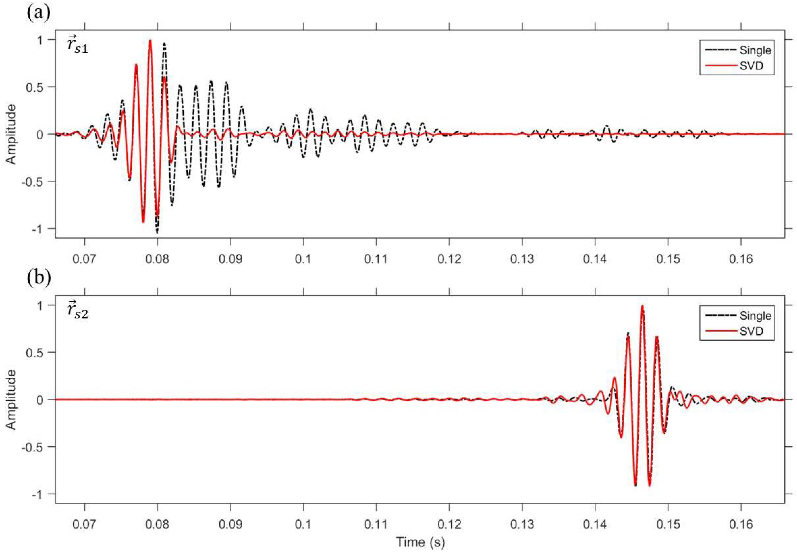
Figure 9.
(Color online) Comparison of VSA-based single TR focusing and VSA-based multiple TR focusing using SVD method in sound speed mismatch environment. Each panel represents a backpropagated field corresponding to a different single snapshot time. Selected locations are = (2.2 km, 20 m) and = (2.3 km, 40 m). (a) VSA-based single TR focusing; (b) VSA-based multiple TR focusing using SVD method.

© 2018 by the authors. Licensee MDPI, Basel, Switzerland. This article is an open access article distributed under the terms and conditions of the Creative Commons Attribution (CC BY) license (http://creativecommons.org/licenses/by/4.0/).
Share and Cite
MDPI and ACS Style
Byun, G.; Song, H.; Kim, J. Virtual Source Array-Based Multiple Time-Reversal Focusing. Appl. Sci. 2018, 8, 99. https://doi.org/10.3390/app8010099
AMA Style
Byun G, Song H, Kim J. Virtual Source Array-Based Multiple Time-Reversal Focusing. Applied Sciences. 2018; 8(1):99. https://doi.org/10.3390/app8010099
Chicago/Turabian StyleByun, Gihoon, Heechun Song, and Jeasoo Kim. 2018. "Virtual Source Array-Based Multiple Time-Reversal Focusing" Applied Sciences 8, no. 1: 99. https://doi.org/10.3390/app8010099
Note that from the first issue of 2016, this journal uses article numbers instead of page numbers. See further details here.