Finite Difference/Collocation Method for a Generalized Time-Fractional KdV Equation


School of Mathematics and Statistics, Central South University, 932 Lushan South Road, Changsha 410083, China
*
Author to whom correspondence should be addressed.
†
These authors contributed equally to this work.
Appl. Sci. 2018, 8(1), 42; https://doi.org/10.3390/app8010042
Submission received: 1 November 2017
/
Revised: 27 December 2017
/
Accepted: 28 December 2017
/
Published: 1 January 2018
Abstract
:In this paper, we studied the numerical solution of a time-fractional Korteweg–de Vries (KdV) equation with new generalized fractional derivative proposed recently. The fractional derivative employed in this paper was defined in Caputo sense and contained a scale function and a weight function. A finite difference/collocation scheme based on Jacobi–Gauss–Lobatto (JGL) nodes was applied to solve this equation and the corresponding stability was analyzed theoretically, while the convergence was verified numerically. Furthermore, we investigated the behavior of solution of the generalized KdV equation depending on its parameter , scale function in fractional derivative. We found that the full discrete scheme was effective to obtain a numerical solution of the new KdV equation with different conditions. The wave number in front of the third order space derivative term played a significant role in splitting a soliton wave into multiple small pieces.
1. Introduction
The study of nonlinear phenomena has always been an active subject in applied science and physics. As a classic nonlinear partial differential equation, the Korteweg-de Vires (KdV) equation is very important in analyzing waves on shallow water surfaces. In history, the KdV equation was first introduced by Boussinesq around 1877, and rediscovered by Diederik Korteweg and Gustav de Vries in 1895 [1]. The KdV equation was firstly derived as an evolution equation that governs small-amplitude, long-surface gravity waves propagating in a shallow channel of water. However, the KdV equation can only be solved analytically in selected initial and boundary conditions due to its nonlinearity [2,3,4,5]. With the development of computational techniques, the KdV equation gained much attention of mathematicians and physicists in the past few years. In [6], by choosing appropriate base functions, a Legendre–Petrov–Galerkin method is applied for the KdV equation. An optimal rate of convergence in -norm is derived without the nonlinear part. By using different test and trial function spaces and basis functions, [7] proposes a new dual-Petrov–Galerkin method for high odd-order differential equations. In [8], pseudo-spectral method is applied to solve the KdV equation, in which the spectral method is implemented parallelled with split-step. This is one of the original results of the pseudo-spectral method applied to the KdV equation. Later in [9], the KdV equation is solved by the homotopy perturbation method. By constructing special forms of initial conditions, numerical solutions expressed by the trigonometric functions, hyperbolic functions are obtained. Many authors applied the collocation method to solve KdV equation due to its high accuracy and good performance in the nonlinear case. In [10], the KdV equation is solved by using the radial basis functions. It is a meshless method based on the collocation with radial basis functions. Five standard radial basis functions are used in the method of the collocation. In [11], A KdV–Burgers equation was discussed by using the modified Bernstein polynomials. The B-polynomials were used to expand the desired solution requiring discretization with only the time variable. The Galerkin method was used to determine the expansion coefficients to construct initial trial functions. A fourth-order Runge–Kutta method was used to solve the system of equations for the time variable. In [12], the sinc-collocation method was applied to solve the nonlinear third-order KdV equation in the space direction with periodic forcing at the boundary numerically and a -weight finite difference method was used to approximate the first-order time derivative. However, all the work above is on the KdV equation with integer-order derivatives. In the recent forty years, many partial differential equations are reconsidered by changing their classical derivative into fractional derivatives.
Fractional derivative is not a new concept. In fact, it was firstly proposed in the discussion of Leibniz and l’Hospital in 1695. Since 1974, when the first international conference of fractional calculus and its application was held, many researchers from scientific and engineering fields brought fractional derivatives back to their research interests. A large number of physical models were renewed by fractional calculus. Under such a background, fractional KdV equation, as well as many other fractional PDEs, are also studied by different methods, either analytical or numerical techniques [13,14,15,16]. In [17], a fractional KdV equation with a Caputo derivative is solved by the Adomian decomposition method. The approximation solution is presented via a convergent series with easily computable components. In [18], based on Maple, the Adomian decomposition method is extended to derive explicit and numerical solutions of the fractional KdV–Burgers equation. In [19], the homotopy analysis method that was developed for integer-order differential equations is directly extended to derive explicit and numerical solutions of the nonlinear fractional KdV equation. In [20], the homotopy perturbation method is implemented to construct solitary solutions for variants of the KdV equations with fractional time derivatives. In this scheme, the solution takes the form of a convergent series, and its terms can be easily calculated via iteration. In a recent work [21], the explicit and approximate solutions of the nonlinear fractional KdV–Burgers equation with time/space-fractional derivatives were presented and discussed. The numerical method is a technique based on the generalized Taylor series formula which constructs an analytical solution in the form of a convergent series. Noting that most of above work is analytical/semianalytical, we are interested in solving the fractional KdV equation numerically by a finite difference/collocation method, and trying to discover some particular features of the soliton solution of the fractional KdV equation.
Fractional derivatives have various definitions, out of which the frequently used ones are defined in Riemann–Liouville and Caputo senses, which can be regarded as a convolution between a fractional power kernel and a function. These kinds of fractional power kernel put more weight in the present than in the past, which is particularly suitable to describe physical processes in the material with short memory, but is incapable of properly describing some behavior observed in materials with huge heterogeneities and structures with different scales. In [22], a new kind of fractional KdV model was established by using the developed Caputo–Fabrizio fractional derivative, and the conditions of existence and uniqueness of the continuous solution were provided. In [23], a time-fractional Shamel–KdV equation with Riesz fractional derivatives was derived to describe nonlinear behavior of dust-ion acoustic waves. In 2012, to unify different existing fractional derivatives, a new fractional calculus was proposed in [24]. Taking a scale function and a weight function into consideration, fractional integrals and derivatives were essentially generalized. Partial differential equations with such generalized fractional derivatives are not studied much [25,26,27,28]. Therefore, in this paper, we choose the KdV equation to further study this topic. By using a generalized derivative with respect to scale function and weight function, we defined a new time-fractional KdV equation. As there is strong nonlinearity in the structure of the KdV equation, the collocation method is applied to the space direction while the finite difference method is implemented in the time direction. Because of the complexity of generalized fractional derivative, some classic mathematical tools are not available anymore in studying the generalized KdV equation, such as variational principle, energy functional, Hölder estimation and Sobolev-type inequalities. We only have very limited methods of theoretical analysis to detect such KdV equations. However, in the current circumstance, the numerical method shall be a useful and direct way to show the details of the considered KdV equation with generalized fractional derivatives. After applying the collocation method in the space direction, the generalized fractional KdV equation is reduced to a nonlinear generalized fractional differential equation with respect to t. Reference [29] studied the existence and uniqueness of a class of generalized fractional boundary value problems by using topological degree theory. In our paper, we focus on numerical methods to analyze such a KdV equation. Thus, we choose initial and boundary conditions that are sufficiently good to guarantee the existence and uniqueness of the new time-fractional KdV equation. We apply a semi-discretization scheme to solve this new fractional KdV. Based on numerical simulation, many new characteristics of the new fractional KdV equation are presented. The remainder of this article is organized as follows: Section 2 is devoted to the preliminaries of generalized fractional calculus. In Section 3, we discuss the numerical scheme and its stability. Two numerical examples are given in Section 4. The first one is calculated to confirm the effectiveness and accuracy of the proposed numerical method. The second one with soliton-type initial condition is used to show important differences between the conventional KdV equation and our generalized fractional KdV equation. Some nonlinear scale functions are considered, which makes the KdV equation more general.
2. Preliminaries of Fractional Calculus and Jacobi Polynomials
2.1. Generalized Fractional Calculus
In this part, we introduce the definitions of new generalized fractional integrals and derivatives. To guarantee that the new generalized fractional integral and derivative are well-defined, we need to assume that the weight function is positive and the scale function is monotonically increasing on the domain.
Definition 1.
([24]) The left-generalized fractional integral of order of a function with respect to a scale function and a weight function is defined as
provided the integral exists. The superscript `*’ indicates the integral here is a new generalized fractional integral.
Definition 2.
([24]) The left first-order generalized derivative of a function with respect to a scale function and a weight function is defined as
provided the right side of the equation is finite.
Definition 3.
([24]) The left-generalized derivative of order m of a function with respect to a scale function and a weight function is defined as
provided the right side of the equation is finite, where m is a positive integer.
Definition 4.
([24]) The left Caputo-type generalized fractional derivative of order of a function with respect to a scale function and a weight function is defined as
provided the right side of the equation is finite, where , m is a positive integer.
Similarly, for one function containing two variables, that is, , its (left) Caputo-type generalized fractional partial derivative with respective to t is defined as [25]
Remark 1.
Left Riemann–Liouville-type generalized fractional derivatives can be defined if we switch the order of integral and differential. When the scale function is selected as and the weight function is a nonzero constant, the operators defined in (1), (4) and left Riemann–Liouville-type generalized fractional derivatives are reduced to left Riemann–Liouville fractional integrals, left Caputo fractional derivatives and left Riemann-Liouville fractional derivatives, respectively.
2.2. Jacobi Polynomials
In recent years, more concentration has been focused on Jacobi polynomials for solving differential equations because the Jacobi parameters and make such polynomials easy to implement. The well-known Jacobi polynomials with indices of degree n are defined on interval and can be expressed as
which are solutions of a class of Sturm–Liouville problems [30].
The integer derivative of on the interval can be represented in the form
Let be a set of Jacobi–Gauss–Lobatto nodes and weights. The corresponding discrete inner product, denoted by , can be defined as
The exactness of the quadratures implies
where is denoted by the space of polynomials whose degree does not exceed .
3. Numerical Scheme and Stability Analysis
The integer-order KdV equation,
is firstly derived to describe one-dimensional shallow-water waves with small but finite amplitudes. Generally, is a positive parameter and indicates the wave number. Replacing the time derivative by the Caputo-type generalized fractional derivative (see (5)), we get
which is called a generalized fractional KdV equation.
Note that the second term of (10) makes it a nonlinear equation. In order to solve this equation, we impose the following initial and boundary conditions
In the following parts, as a premise, we make an assumption that the problem (10) and (11) is well-posed.
3.1. Numerical Discretization in the Time Direction
To establish a numerical approximation scheme in the time direction, we divide the time domain into M equal parts, where M is a positive integer. Thus is the time-grid size. We label the successive time nodes as , where is the initial time. Assuming and is strictly monotonic increasing on , then by setting . The Caputo-type generalized fractional derivative of can be discretized as
where
and is the truncation error given by
Lemma 1.
Proof.
According to the mean-value theorem of integrals, there exist such that
Since is monotonically increasing, it follows that and . ☐
Remark 2.
To analyze the truncation error , we denote for , and for convenience. By using the Newton interpolation method, we interpolate on as
and according to the theory of Newton interpolation, there exists such that
Then, (14) can be rewritten as
Thus,
Denote as the interval satisfying , then the truncation error (14) has the form
when satisfies the Lipschitz condition on and L is the Lipschitz constant.
3.2. Numerical Discretization in the Space Direction
As the homogeneous Neumann condition is included in the boundary conditions, we choose a type of polynomial as to approximate to the in the space direction. In our problem, we set that is a combination of Jacobi polynomials of degree , and satisfies the Equation (10) exactly at , and boundary condition at and . are Jacobi–Gauss–Lobatto (JGL) nodes on by introducing the change of variable
where , are JGL points on [−1, 1]. Based on the analysis above, we take
as the basis functions in the space direction. Then, the numerical solution of problem (10) has the form:
satisfying
for any . Substituting (24) to the semi-discretization (22), we have
where and is the error in the space direction caused by replacing with . The classical first- and third-order partial derivatives in (27) are derived as
Neglecting the error parts, we obtain the full discretization scheme of Equation (10). For , it holds that
where
3.3. Stability Analysis
Firstly, we consider the linear case of the generalized fractional KdV equation as
and similarly, we discretize the linear case as
Now we state our main theorem as follows.
Theorem 1.
Assume that is a continuous function satisfying boundary conditions (11) for any t, and is continuous function. Letting is the numerical solution of discrete scheme (33), the scheme (33) is stable unconditionally and for any , it holds that
where .
Proof.
Let , and is a polynomial of degree satisfying . The discrete form (30) at JGL nodes can be rewritten as
Multiplying both sides of (35) by and summing for j from 0 to N leads to
where is the corresponding weight. Since the degrees of , and are not exceeding , according to (8), they can be exactly expressed by the Jacobi–Gauss–Lobatto quadrature:
It is straightforward to show that
and
which yields
by applying Cauchy–Schwartz inequality and Lemma 1.
In the following, we will continue our proof by induction. Obviously, (34) holds when according to (42):
Assuming that (34) is valid for any , it is easy to verify from (42) that
This completes the proof. ☐
Remark 3.
For the nonlinear case (10), at every collocation node , we have the ’frozen coefficient’ . Since Theorem 1 is sustained for any constant ξ, the discretization scheme (30) is stable by regarding as a constant coefficient.
4. Numerical Results and Analysis
In Section 3.3, we proved the stability of the proposed scheme in the linear case. Following numerical examples will show that our algorithm is also available in the nonlinear case. In this part, two numerical examples are provided to demonstrate the effectiveness of the finite difference/collocation scheme. The initial and boundary conditions are given to establish an exact solution in the first example to analyze error and convergence numerically. In the second example, the initial condition is taken as a hyperbolic sine function and the boundary condition is homogenous. For convenience, we take the weight function in the following part.
Example 1.
Consider the generalized fractional KdV Equation (10) with following initial and boundary conditions
With the above conditions, by taking
the problem (10) has the exact solution of form
Here, we choose , , and for , for , and for , respectively. When , the generalized fractional derivative in (10) is the classical Caputo fractional derivative.
Figure 1 shows the numerical solutions and the distribution of absolute error when , and . Note that numerical solutions are highly aligned with exact solutions.
With the computer of 1.8 GHz Intel Core i5 and 8 GB 1600 MHz DDR3, Table 1, Table 2 and Table 3 list maximal absolute errors (MAE), convergence order (CO) and elapsed time with three different scale functions: , and . Results show that the convergence order under different scale functions increases as the fractional derivative order decreases, and is close to .
Example 2.
Applying the proposed finite difference/collocation scheme, we obtain the numerical solutions over the domain under different situations. Firstly, letting , the generalized fractional derivative in (10) is equivalent to the Caputo fractional derivative. Figure 2 shows the influence of and under conditions of , . By fixing , diffusion processes with and are illustrated. It is shown that when is small, the soliton (initial condition) will be decomposed to neighboring solitons, whose amplitudes are affected by the fractional derivative . This decomposing phenomenon cannot be observed when becomes larger. In the case of , the soliton wave does not move much with as expected, and with the decreasing of , the amplitudes are getting smaller.
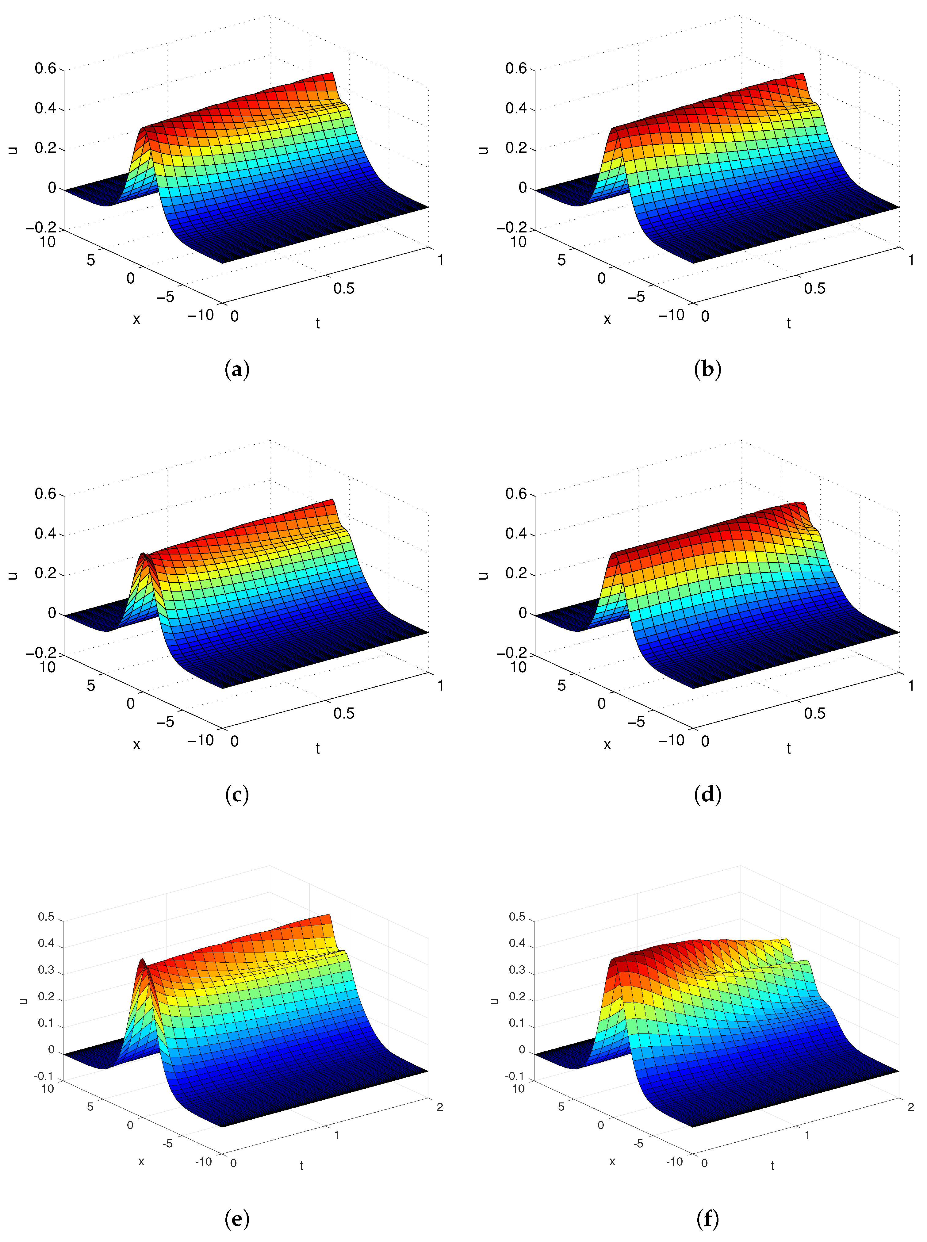
Next, numerical results with different scale functions , t , and are shown in Figure 3 when . Denoting , , scale function behaves like a “contracting function” for the time variable over domain when , while behaving like a “stretching function” as (see [25]). From Figure 3, when , decomposing and diffusion phenomena appeared earlier in contrast with the case when , just like being contracted. On the contrary, the decomposing process works quite slowly when . Moreover, the speed of decomposing is slower as s becomes larger. However, comparing with Figure 2a, Figure 3e,f shows that when , with the increasing of s, the speed of decomposing is getting faster.
5. Conclusions
We numerically study a new class of KdV equation, in which the partial derivative on the time variable is defined by a new generalized fractional derivative. The finite difference method is applied to solve the generalized fractional KdV equation under different selections of parameter, order of fractional derivatives and initial conditions. The stability of the numerical scheme is verified and the order of convergence is evaluated numerically in cases of different scale functions. Numerical examples are provided to demonstrate the effectiveness and accuracy of the numerical scheme. Furthermore, we investigate the dynamics of soliton solution in the generalized fractional KdV equation via simulation. We find that the number and amplitude of waves are significantly influenced by the parameter in the equation and the order of fractional derivatives.
Acknowledgments
This work was partly supported by the National Key Research an Development Program of China (No. 2017YFB0701700), the NSFC (No. 11501581, No. 51134003, No. 51174236), the Research Project (No. 502042032) of Central South University, the Project funded by China Postdoctoral Science Foundation (No. 2015M570683), the Project supported by the National Basic Research Development Program of China (No. 2011CB606306), the project supported by the National Key Laboratory Open Program of Porous metal material of China (No. PMM-SKL-4-2012).
Author Contributions
Wen Cao conceived and designed the experiments; Wen Cao and Yufeng Xu analyzed the data; Zhoushun Zheng contributed analysis tools; Wen Cao, Yufeng Xu and Zhoushun Zheng wrote the paper.
Conflicts of Interest
The authors declare no conflict of interest.
References
- Korteweg, D.J.; de Vries, G. On the change of form of long waves and advancing in a rectangular canal and on a new type of long stationary waves. Philos. Mag. 1895, 39, 422–443. [Google Scholar] [CrossRef]
- Tian, B.; Gao, Y.-T. Exact solutions for the Bogoyavlenskii coupled KdV equations. Phys. Lett. A 1995, 208, 193–196. [Google Scholar] [CrossRef]
- Vlieg-Hulstman, M.; Halford, W.D. Exact solutions to KdV equations with variable coefficients and/or nonuniformities. Comput. Math. Appl. 1995, 29, 39–47. [Google Scholar] [CrossRef]
- Senthilkumaran, M.; Pandiaraja, D.; Vaganan, B.M. New exact explicit solutions of the generalized KdV equations. Appl. Math. Comput. 2008, 202, 693–699. [Google Scholar] [CrossRef]
- Akdi, M.; Sedra, M.B. Numerical KdV equation by the adomian decomposition method. Am. J. Mod. Phys. 2013, 2, 111–115. [Google Scholar] [CrossRef]
- Ma, H.; Sun, W. A Legendre-Petrov-Galerkin and Chebyshev collocation method for third-order differential equations. SIAM J. Numer. Anal. 2000, 38, 1425–1438. [Google Scholar] [CrossRef]
- Shen, J. A new Dual-Petrov-Galerkin method for third and high odd-order differential equations: Application to the KdV equation. SIAM J. Numer. Anal. 2003, 41, 1595–1619. [Google Scholar] [CrossRef]
- Guo, J.; Taha, T.R. Parallel implementation of the split-step and the pseudospectral methods for solving higher KdV equation. Math. Comput. Simul. 2003, 62, 41–51. [Google Scholar] [CrossRef]
- An, H.; Chen, Y. Numerical complexiton solutions for the complex KdV equation by the homotopy perturbation method. Appl. Math. Comput. 2008, 203, 125–133. [Google Scholar] [CrossRef]
- Dag, I.; Dereli, Y. Numerical solutions of KdV equation using radial basis functions. Appl. Math. Model. 2008, 32, 535–546. [Google Scholar] [CrossRef]
- Bhatta, D. Use of modified Bernstein polynomials to solve KdV-Burgers equation numerically. Appl. Math. Comput. 2008, 206, 457–464. [Google Scholar] [CrossRef]
- Al-Khaled, K.; Haynes, N.; Schiesser, W.; Usman, M. Eventual periodicity of the forced oscillations for a Korteweg-de Vries type equation on a bounded domain using a sinc collocation method. J. Comput. Appl. Math. 2018, 330, 417–428. [Google Scholar] [CrossRef]
- Xu, Y.; He, Z. The short memory principle for solving Abel differential equation of fractional order. Comput. Math. Appl. 2011, 62, 4796–4805. [Google Scholar] [CrossRef]
- Xu, Q.; Hesthaven, J.S. Stable multi-domain spectral penalty methods for fractional partial differential equations. J. Comput. Phys. 2014, 257, 241–258. [Google Scholar] [CrossRef]
- Zhao, X.; Xu, Q. Efficient numerical schemes for fractional sub-diffusion equation with the spatially variable coefficient. Appl. Math. Model. 2014, 38, 3848–3859. [Google Scholar] [CrossRef]
- Xu, Q.; Hesthaven, J.S. Discontinuous Galerkin method for fractional convection-diffusion equations. SIAM J. Numer. Anal. 2014, 52, 405–423. [Google Scholar] [CrossRef]
- Momani, S. An explicit and numerical solutions of the fractional KdV equation. Math. Comput. Simul. 2005, 70, 110–118. [Google Scholar] [CrossRef]
- Wang, Q. Numerical solutions for fractional KdV-Burgers equation by Adomian decomposition method. Appl. Math. Comput. 2006, 182, 1048–1055. [Google Scholar]
- Song, L.; Zhang, H. Application of homotopy analysis method to fractional KdV-Burgers-Kuramoto equation. Phys. Lett. A 2007, 367, 88–94. [Google Scholar] [CrossRef]
- Odibat, Z.M. Exact solitary solutions for variants of the KdV equations with fractional time derivatives. Chaos Soliton Fractal 2009, 40, 1264–1270. [Google Scholar] [CrossRef]
- El-Ajou, A.; Arqub, O.A.; Momani, S. Approximate analytical solution of the nonlinear fractional KdV-Burgers equation: A new iterative algorithm. J. Comput. Phys. 2015, 293, 81–95. [Google Scholar] [CrossRef]
- Doungmo Goufo, E.F. Application of the Caputo-Fabrizio fractional derivative without singular kernel to Korteweg-de Vries-Burgers Equation. Math. Model. Anal. 2016, 21, 188–198. [Google Scholar] [CrossRef]
- Guo, S.; Mei, L.; He, Y.; Li, Y. Time-fractional Schamel–KdV equation for dust-ion-acoustic waves in pair-ion plasma with trapped electrons and opposite polarity dust grains. Phys. Lett. A 2016, 380, 1031–1036. [Google Scholar] [CrossRef]
- Agrawal, O.P. Some generalized fractional calculus operators and theeir applications in integral equations. Fract. Calc. Appl. Anal. 2012, 15, 700–711. [Google Scholar] [CrossRef]
- Xu, Y.; Agrawal, O.P. Numerical solutions and analysis of diffusion for new generalized fractional Burgers equation. Fract. Calc. Appl. Anal. 2013, 16, 709–736. [Google Scholar] [CrossRef]
- Xu, Y.; He, Z.; Agrawal, O.P. Numerical and analytical solutions of new generalized fractional diffusion equation. Comput. Math. Appl. 2013, 66, 2019–2029. [Google Scholar] [CrossRef]
- Xu, Y.; Agrawal, O.P. Numerical solutions and analysis of diffusion for new generalized fractional advection-diffusion equations. Cent. Eur. J. Phys. 2013, 11, 1178–1193. [Google Scholar] [CrossRef]
- Xu, Y.; Agrawal, O.P. Models and numerical solutions of generalized oscillator equations. J. Vib. Acoust. 2014, 136, 50903. [Google Scholar] [CrossRef]
- Cao, W.; Xu, Y.; Zheng, Z. Existence results for a class of generalized fractional boundary value problem. Adv. Differ. Equ. 2017, in press. [Google Scholar] [CrossRef]
- Shen, J.; Tang, T.; Wang, L.-L. Spectral Methods; Springer: Berlin/Heidelberg, Germany, 2011. [Google Scholar]
Figure 1.
Numerical solutions and error distribution of Example 1. (a) Numerical solutions; (b) distribution of absolute error.
Figure 1.
Numerical solutions and error distribution of Example 1. (a) Numerical solutions; (b) distribution of absolute error.
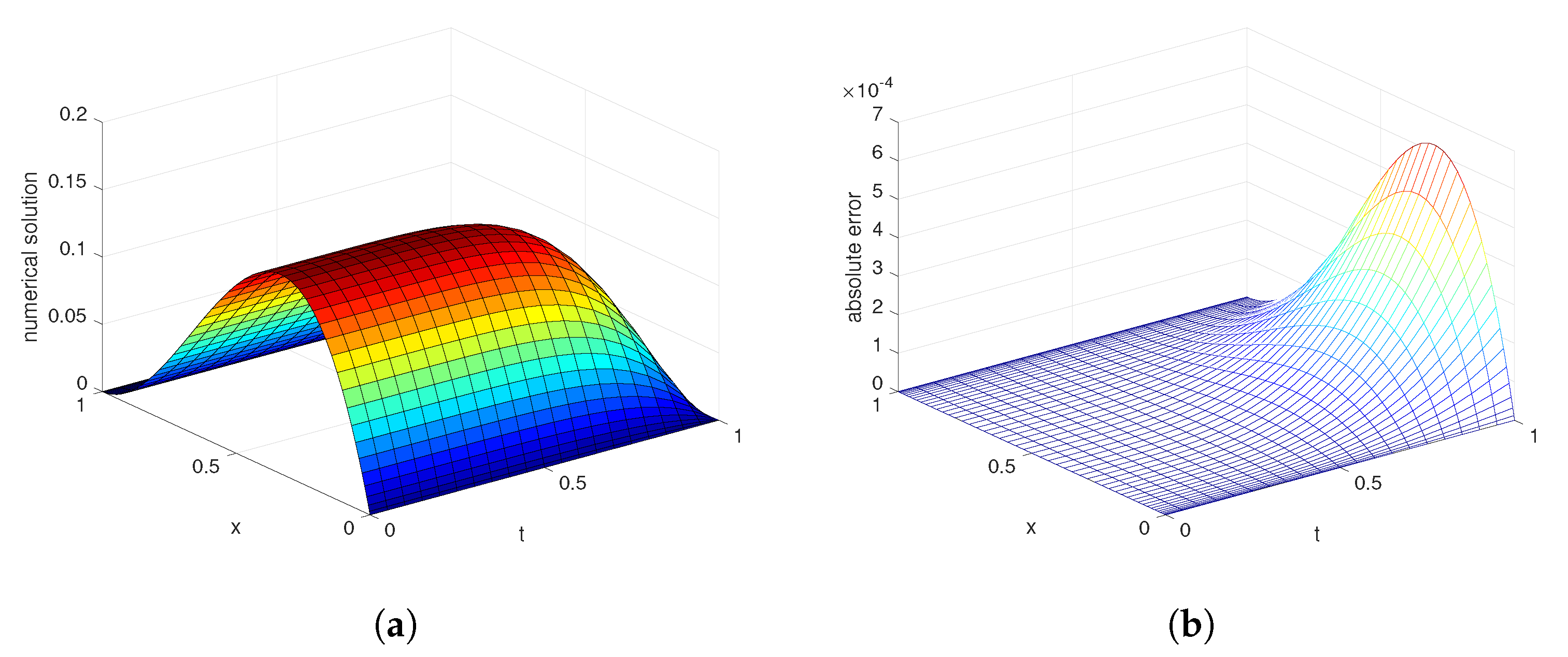
Figure 2.
The effect of and of Example 2 when . (a) ; (b) ; (c) ; (d) .
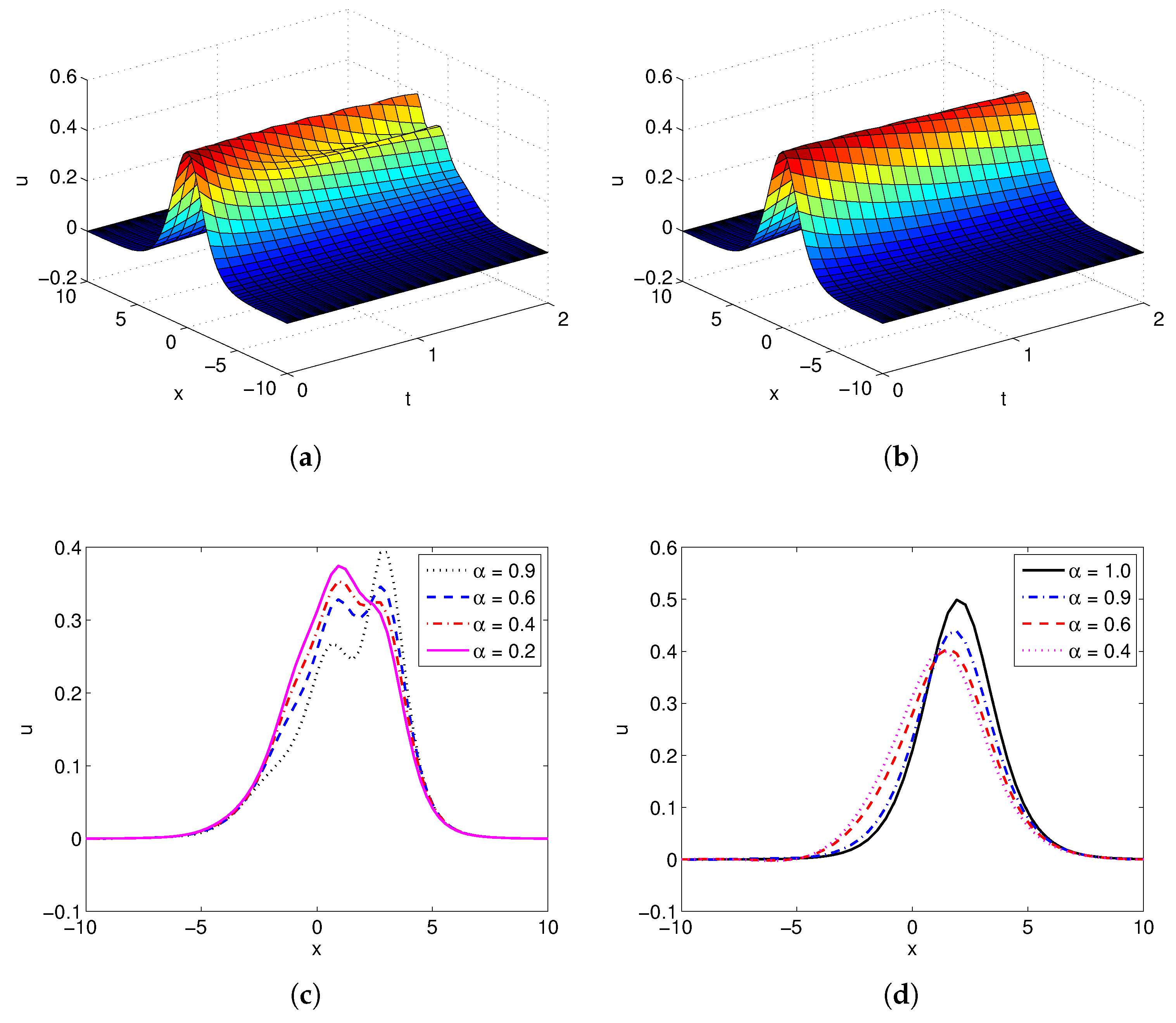
Figure 3.
The influence of of Example 2 with and . (a) ; (b) ; (c) ; (d) ; (e) ; (f) .


Table 1.
The maximal absolute error (MAE) and convergence order (CO) for Example 1 when .
| M | |||||||||
|---|---|---|---|---|---|---|---|---|---|
| MAE | CO | Time | MAE | CO | Time | MAE | CO | Time | |
| 100 | 1.39 × | - | 7.9 s | 2.67 × | - | 7.1 s | 1.71 × | - | 7.4 s |
| 200 | 4.28 × | 1.70 | 18.7 s | 1.03 × | 1.37 | 17.6 s | 8.04 × | 1.09 | 17.9 s |
| 300 | 2.13 × | 1.72 | 32.1 s | 5.89 × | 1.38 | 30.3 s | 5.16 × | 1.09 | 31.7 s |
| 400 | 1.29 × | 1.73 | 46.3 s | 3.95 × | 1.38 | 47.6 s | 3.76 × | 1.10 | 47.2 s |
Table 2.
The maximal error and convergence order for Example 1 when .
| M | |||||||||
|---|---|---|---|---|---|---|---|---|---|
| MAE | CO | Time | MAE | CO | Time | MAE | CO | Time | |
| 100 | 1.77 × | - | 7.9 s | 4.38 × | - | 7.6 s | 3.35 × | - | 7.5 s |
| 200 | 5.42 × | 1.70 | 17.8 s | 1.69 × | 1.37 | 18.2 s | 1.58 × | 1.09 | 17.3 s |
| 300 | 2.70 × | 1.72 | 33.4 s | 9.66 × | 1.38 | 30.9 s | 1.01 × | 1.09 | 30.6 s |
| 400 | 1.64 × | 1.73 | 52.16 s | 6.48 × | 1.39 | 55.4 s | 7.38 × | 1.09 | 51.8 s |
Table 3.
The maximal error and convergence order for Example 1 when .
| M | |||||||||
|---|---|---|---|---|---|---|---|---|---|
| MAE | CO | Time | MAE | CO | Time | MAE | CO | Time | |
| 100 | 9.64 × | - | 7.5 s | 1.43 × | - | 7.5 s | 7.52 × | - | 7.3 s |
| 200 | 2.96 × | 1.70 | 18.2 s | 5.50 × | 1.37 | 16.9 s | 3.54 × | 1.09 | 17.6 s |
| 300 | 1.48 × | 1.72 | 31.8 s | 3.14 × | 1.38 | 29.8 s | 2.27 × | 1.09 | 29.7 s |
| 400 | 8.99 × | 1.72 | 46.1 s | 2.11 × | 1.39 | 48.2 s | 1.66 × | 1.10 | 49.1 s |
© 2018 by the authors. Licensee MDPI, Basel, Switzerland. This article is an open access article distributed under the terms and conditions of the Creative Commons Attribution (CC BY) license (http://creativecommons.org/licenses/by/4.0/).
Share and Cite
MDPI and ACS Style
Cao, W.; Xu, Y.; Zheng, Z. Finite Difference/Collocation Method for a Generalized Time-Fractional KdV Equation. Appl. Sci. 2018, 8, 42. https://doi.org/10.3390/app8010042
AMA Style
Cao W, Xu Y, Zheng Z. Finite Difference/Collocation Method for a Generalized Time-Fractional KdV Equation. Applied Sciences. 2018; 8(1):42. https://doi.org/10.3390/app8010042
Chicago/Turabian StyleCao, Wen, Yufeng Xu, and Zhoushun Zheng. 2018. "Finite Difference/Collocation Method for a Generalized Time-Fractional KdV Equation" Applied Sciences 8, no. 1: 42. https://doi.org/10.3390/app8010042
Note that from the first issue of 2016, this journal uses article numbers instead of page numbers. See further details here.