A Semi-Explicit Multi-Step Method for Solving Incompressible Navier-Stokes Equations

Abstract

The fractional step method is a technique that results in a computationally-efficient implementation of Navier–Stokes solvers. In the finite element-based models, it is often applied in conjunction with implicit time integration schemes. On the other hand, in the framework of finite difference and finite volume methods, the fractional step method had been successfully applied to obtain predictor-corrector semi-explicit methods. In the present work, we derive a scheme based on using the fractional step technique in conjunction with explicit multi-step time integration within the framework of Galerkin-type stabilized finite element methods. We show that under certain assumptions, a Runge–Kutta scheme equipped with the fractional step leads to an efficient semi-explicit method, where the pressure Poisson equation is solved only once per time step. Thus, the computational cost of the implicit step of the scheme is minimized. The numerical example solved validates the resulting scheme and provides the insights regarding its accuracy and computational efficiency.

1. Introduction

The solution of incompressible flow problems arising in real-life engineering applications calls for developing accurate, yet efficient schemes, as the associated computational time becomes a decisive factor for their use. Among the many methods available, one class of techniques commonly implemented is the well-known fractional step method.

The method was originally introduced in the works of Chorin [1] and Temam [2] for incompressible Navier–Stokes equations (independently, a similar methodology was developed and thoroughly studied by Yanenko [3,4]).

Basically, the method allows one to decouple the primary variables of the governing equations (the velocity and the pressure) and replaces the “monolithic” solution of the original coupled system by a series of solution steps, ensuring that only one variable (either the velocity or the pressure) is unknown at each step. First, the momentum equation is solved for an intermediate, non-solenoidal, velocity removing the dependence on the unknown pressure. Afterwards, the pressure is found, and the velocity is corrected fulfilling the incompressibility constraint.

It has been shown that the fractional step method can be viewed as a block LU decomposition of the original monolithic equations system [5]. The method is very popular due to the resulting computational efficiency (see, e.g., [6,7,8]). The accuracy of the method was addressed in [9]. Error estimates and pressure stability issues of the fractional step method have been analyzed in [10]. An exhaustive review of different implementation versions of the method can be found in [11]. A method that unifies the artificial compressibility approach and a fractional step method can be consulted in [12]. The fractional step methodology has been also applied to compressible flows modeling (see, e.g., [13,14]). The peculiarities of applying the fractional step method to multiphase flows with surface tension effects have been highlighted in [15].

While the majority of works on fractional step methods had been carried out considering fixed-grid (Eulerian) approaches, some recent works have analyzed the implications of applying the fractional step method to moving grid (Lagrangian) methods [16,17]. The fractional step method has been also applied for modeling incompressible solids [18].

In the context of incompressible flow modeling, the fractional step method is often applied in conjunction with implicit time integration schemes. This is the case for all the above-mentioned works. Purely explicit schemes cannot be applied to incompressible Navier–Stokes equations due to the implicit nature of the pressure.

On the other hand, an appealing possibility consists of developing a semi-explicit scheme, where velocity is integrated explicitly, while pressure is treated implicitly. A particularly appealing option relies on adopting an accurate high order methodology such as the Runge–Kutta time integration family. This has been followed in several works, e.g., [19,20,21,22,23,24,25,26].

In the context of finite volume methods, this was followed, e.g., in [21,22]. In [21], the accuracy of different versions of Runge–Kutta schemes is analyzed. The authors derive a predictor-corrector scheme, which is very similar to a fractional step one; however, no spitting error is committed as pressure is computed at every sub-step of the Runge–Kutta scheme. In [22], stability bounds of different fractional step-based schemes (including the ones using Runge–Kutta integration) are analyzed for high Reynolds number flows.

Several authors developed semi-explicit Runge–Kutta-based methods in the context of the finite difference framework. In [22], a third-order Runge–Kutta scheme for the convective term combined with a Crank–Nicholson integration for the viscous term was proposed. In [23], a fourth-order Runge–Kutta scheme equipped with the solution of the pressure Poisson equation at each sub-step is proposed (similar to [21]). The above-mentioned semi-explicit finite volume and finite differences approaches rely on solving the pressure Poisson equation at every sub-step of the multi-step scheme, which is a computationally-intensive option. The idea of reducing the number of implicit steps of a semi-explicit scheme has been proposed in [25]. In the finite difference context, the authors proposed a semi-explicit third-order Runge–Kutta-based scheme where the convective term was advanced explicitly, while treating the viscous term implicitly. Most importantly, they suggested assuming that the pressure corresponding to the intermediate Runge–Kutta steps equals the historical one. Thus, the computationally-expensive pressure Poisson equation was solved only once per time step.

In the present work, we develop a similar approach in the context of Galerkin finite element methods. In this work, we derive a scheme based on the combination of the fractional step technique with the fourth-order Runge–Kutta scheme, striving to minimize the computational cost corresponding to the implicit steps. We show that a certain assumption regarding the intermediate step pressures results in an efficient semi-explicit scheme that requires solving the pressure Poisson equation only once per time step.

The paper is organized as follows. We first define the space-discrete problem considering linear velocity-pressure stabilized finite elements. Afterwards, time-discrete equations using the fourth-order Runge–Kutta scheme are derived. Next, assumptions for the pressure at intermediate Runge–Kutta steps are introduced, and the fractional split is applied. The resulting semi-explicit scheme is obtained. The paper concludes with a numerical verification example. Time accuracy and computational efficiency of the method are estimated.

2. Governing Equations

The Navier–Stokes equations for incompressible flow defined over domain $\mathrm{\Omega }$ with boundary $\mathrm{\Gamma }$ can be written as:

$$\begin{array}{c}\hfill \rho \frac{\partial \mathbf{u}}{\partial t}+\rho (\mathbf{u}·\nabla )\mathbf{u}-\rho \nu \Delta \mathbf{u}+\nabla p=\mathbf{f},\end{array}$$

(1)

$$\begin{array}{c}\hfill \nabla ·\mathbf{u}=0,\end{array}$$

(2)

where $\mathbf{u}$ is the velocity vector, p the pressure, t time, $\mathbf{f}$ the body force, $\rho$ the density and $\nu$ the kinematic viscosity.

For ensuring the well-posedness of the system defined by Equations (1) and (2), suitable boundary conditions must be specified. On the boundary $\mathrm{\Gamma }={\mathrm{\Gamma }}_D\cup {\mathrm{\Gamma }}_N$, such that ${\mathrm{\Gamma }}_D\cap {\mathrm{\Gamma }}_N=\varnothing$, the following conditions are prescribed:

$$\begin{array}{cc}\hfill \mathbf{u}={\mathbf{u}}^{pr}& \mathrm{at}{\mathrm{\Gamma }}_D,\hfill \end{array}$$

(3)

$$\begin{array}{cc}\hfill \sigma ·\mathbf{n}={\sigma }_n^{pr}& \mathrm{at}{\mathrm{\Gamma }}_N,\hfill \end{array}$$

(4)

where ${\mathbf{u}}^{pr}$ is the prescribed velocity, $\mathbf{n}$ is the outer unit normal to ${\mathrm{\Gamma }}_N$ and ${\sigma }_n^{pr}$ is the prescribed traction vector. Homogeneous boundary conditions will be considered here for the sake of simplicity.

We define symbolically the differential Navier–Stokes operator as:

$$\mathcal{A}(\mathbf{u},p)=\left(\begin{array}{c}{\mathcal{A}}_1(\mathbf{u},p)\\ {\mathcal{A}}_2(\mathbf{u},p)\end{array}\right),$$

(5)

where:

$${\mathcal{A}}_1=\rho (\mathbf{u}·\nabla )\mathbf{u}-\rho \nu \Delta \mathbf{u}+\nabla p,$$

(6)

$${\mathcal{A}}_2=\nabla ·\mathbf{u}.$$

(7)

Then, introducing the notation $\mathcal{F}=\left(\begin{array}{c}\mathbf{f}\\ 0\end{array}\right)$, the governing equations can be written as:

$$\left(\begin{array}{c}\rho \frac{\partial \mathbf{u}}{\partial t}\\ 0\end{array}\right)+\mathcal{A}(\mathbf{u},p)=\mathcal{F}.$$

(8)

2.1. Space Discretization

The Galerkin weak form of (8) reads:

$$\left(\mathit{\omega },\rho \frac{\partial \mathbf{u}}{\partial t}\right)+(\mathit{\omega },{\mathcal{A}}_1)+(q,{\mathcal{A}}_2)=\langle \mathit{\omega },\mathbf{f}\rangle ,$$

(9)

where $\mathit{\omega }$ and q are the velocity and pressure test functions. In the notation adopted, $(·,·)$ and $\langle ·,·\rangle$ stand for a bilinear and linear forms, respectively.

In order to obtain stable solutions for convection-dominated flows, the equations must be stabilized. Additionally, pressure stabilization is necessary for equal order velocity-pressure interpolations, as they do not satisfy the compatibility condition [27]. The Galerkin/least squares (GLS) stabilization method allows one to circumvent this problem by summing ${\sum }_n{\int }_{\mathrm{\Omega }}\mathcal{A}(\mathit{\omega },q)·(\mathcal{F}-\mathcal{A}(\mathbf{u},p)-\frac{\partial \mathbf{u}}{\partial t})$ to the original weak form of the problem [28]. This means summing the product of the residual with the Navier–Stokes operator $\mathcal{A}(\mathit{\omega },q)$ (this operator may be viewed as a changed weight function). We note that for linear velocity-pressure elements, the GLS method coincides with the more recent (and less diffusive for a general case) algebraic sub-grid scale (ASGS) method [29], the latter being defined based on the adjoint operator ${\mathcal{A}}^{*}$ as a weight function for the residual.

Summing up the Galerkin weak form with the stabilization terms results in:

$$\begin{array}{c}\rho (\mathit{\omega },\frac{\partial \mathbf{u}}{\partial t})+\rho (\mathit{\omega },\mathbf{u}·\nabla \mathbf{u})+(\mathit{\omega },\nabla p)-\rho \nu (\mathit{\omega },\Delta \mathbf{u})+(q,\nabla ·\mathbf{u})+\\ \sum _{el}\tau {\int }_{{\mathrm{\Omega }}_{el}}\left(\nabla q+\rho \mathit{\omega }·\nabla \mathit{\omega }-\rho \nu \Delta \mathit{\omega }\right)(\mathbf{f}-\rho \frac{\partial \mathbf{u}}{\partial t}-\rho \mathbf{u}·\nabla \mathbf{u}+\rho \nu \Delta \mathbf{u}-\nabla p),\end{array}$$

(10)

where the stabilization coefficient $\tau$ is defined as (see, e.g., [28]):

$$\tau =\frac{2\left|\right|\mathbf{u}\left|\right|}{h}+\frac{4\nu }{h^2},$$

(11)

where h is the element size.

Integrating the viscous term by parts and rearranging the terms (noting that in Equation (10), products containing the test function $\mathit{\omega }$ contribute to the momentum equation, while the ones containing q contribute to the mass conservation equation), the modified linear momentum and mass conservation equations are obtained:

$$\begin{array}{c}\rho (\mathit{\omega },\frac{\partial \mathbf{u}}{\partial t})+\rho (\mathit{\omega },\mathbf{u}·\nabla \mathbf{u})+\rho \nu (\nabla \mathit{\omega },\nabla \mathbf{u})-(\nabla ·\mathit{\omega },p)+\\ \sum _{el}\tau {\int }_{{\mathrm{\Omega }}_{el}}\left(\mathit{\omega }·\nabla \mathit{\omega }\right)\left(\mathbf{f}-\rho \frac{\partial \mathbf{u}}{\partial t}-\rho \mathbf{u}·\nabla \mathbf{u}-\nabla p\right)=\langle \mathbf{f},\mathit{\omega }\rangle ,\end{array}$$

(12)

$$(q,\nabla ·\mathbf{u})+\sum _{el}\tau {\int }_{{\mathrm{\Omega }}_{el}}\nabla q\left(\mathbf{f}-\rho \frac{\partial \mathbf{u}}{\partial t}-\rho \mathbf{u}·\nabla \mathbf{u}-\nabla p\right)=0.$$

(13)

Prior to establishing the space-discretized stabilized governing system, we define the matrices and vectors corresponding to each term of Galerkin weak form:

$$(\mathit{\omega },\mathbf{u})⟶\mathbf{M}\overline{\mathbf{u}},$$

(14)

$$(\nabla ·\mathit{\omega },p)⟶\mathbf{G}\overline{\mathbf{p}},$$

(15)

$$(\nabla \mathit{\omega },\nabla \mathbf{u})⟶\mathbf{L}\overline{\mathbf{u}},$$

(16)

$$\left(\mathit{\omega },\left(\mathbf{u}·\nabla \mathbf{u}\right)\right)⟶\mathbf{C}(\overline{\mathbf{u}})\overline{\mathbf{u}},$$

(17)

$$\langle \mathbf{f},\mathit{\omega }\rangle ⟶\mathbf{F}.$$

(18)

The operators corresponding to the stabilization terms are:

$$\sum _{el}\tau {\int }_{{\mathrm{\Omega }}_{el}}(\mathit{\omega }·\nabla \mathit{\omega })(\mathit{\omega }·\nabla \mathbf{u})⟶{\mathbf{S}}_1\overline{\mathbf{u}},$$

(19)

$$\sum _{el}\tau {\int }_{{\mathrm{\Omega }}_{el}}(\mathit{\omega }·\nabla \mathit{\omega })(\mathbf{u})⟶{\mathbf{S}}_2\overline{\mathbf{u}},$$

(20)

$$\sum _{el}\tau {\int }_{{\mathrm{\Omega }}_{el}}(\mathit{\omega }·\nabla \mathit{\omega })(\nabla p)⟶{\mathbf{S}}_3\overline{\mathbf{p}},$$

(21)

$$\sum _{el}\tau {\int }_{{\mathrm{\Omega }}_{el}}(\mathit{\omega }·\nabla \mathit{\omega })(\frac{\partial \mathbf{u}}{\partial t})⟶{\mathbf{M}}_{st}\frac{\partial \overline{\mathbf{u}}}{\partial t},$$

(22)

$$\sum _{el}\tau {\int }_{{\mathrm{\Omega }}_{el}}(\mathit{\omega }·\nabla \mathit{\omega })(\mathbf{f})⟶{\mathbf{F}}_{s1},$$

(23)

$$\sum _{el}\tau {\int }_{{\mathrm{\Omega }}_{el}}(\nabla q)(\mathbf{f})⟶{\mathbf{F}}_{s2},$$

(24)

$$\sum _{el}\tau {\int }_{{\mathrm{\Omega }}_{el}}(\nabla q)(\mathbf{u})⟶{\mathbf{S}}_4\overline{\mathbf{u}},$$

(25)

$$\sum _{el}\tau {\int }_{{\mathrm{\Omega }}_{el}}(\nabla q)((\mathit{\omega }·\nabla )\mathbf{u})⟶{\mathbf{S}}_5\overline{\mathbf{u}},$$

(26)

$$\sum _{el}\tau {\int }_{{\mathrm{\Omega }}_{el}}(\nabla q)(\nabla p)⟶{\mathbf{L}}_{\tau }\overline{\mathbf{p}}.$$

(27)

Note that the variables distinguished by an over-bar ($\overline{\mathbf{u}}$ and $\overline{\mathbf{p}}$) stand for vectors of nodal quantities.

Stabilized space-discrete equations in matrix form read:

$$\begin{array}{c}\hfill \left(\mathbf{M}+{\mathbf{M}}_{st}\right)\frac{\partial \overline{\mathbf{u}}}{\partial t}+(\mu \mathbf{L}+\mathbf{C}(\overline{\mathbf{u}})+{\mathbf{S}}_1+{\mathbf{S}}_2)\overline{\mathbf{u}}-(\mathbf{G}+{\mathbf{S}}_3)\overline{\mathbf{p}}=\mathbf{F}+{\mathbf{F}}_{s1},\end{array}$$

(28)

$$\begin{array}{c}\hfill (\mathbf{D}+{\mathbf{S}}_4+{\mathbf{S}}_5)\overline{\mathbf{u}}+{\mathbf{L}}_{\tau }\overline{\mathbf{p}}={\mathbf{F}}_{s2}.\end{array}$$

(29)

Note that dynamic viscosity $\mu =\rho \nu$ was used. In the scope of applying the time integration scheme of an explicit type, the lumped form of the mass matrix is adopted.

For the sake of clarity, we shall introduce the following short-hand notation:

$$\begin{array}{c}\hfill \overline{\mathbf{C}}=\mathbf{C}+\mu \mathbf{L}+{\mathbf{S}}_1+{\mathbf{S}}_2,\end{array}$$

(30)

$$\begin{array}{c}\hfill \overline{\mathbf{G}}={\mathbf{S}}_3+\mathbf{G},\end{array}$$

(31)

$$\begin{array}{c}\hfill \overline{\mathbf{F}}=\mathbf{F}+{\mathbf{F}}_{s1}+{\mathbf{M}}_{st}{\overline{\mathbf{a}}}_n,\end{array}$$

(32)

$$\begin{array}{c}\hfill \overline{\mathbf{D}}=\mathbf{D}+{\mathbf{S}}_4+{\mathbf{S}}_5,\end{array}$$

(33)

$$\begin{array}{c}\hfill \widehat{\mathbf{F}}={\mathbf{F}}_{s2},\end{array}$$

(34)

$$\begin{array}{c}\hfill \overline{\mathbf{M}}=\mathbf{M}+{\mathbf{M}}_{st}.\end{array}$$

(35)

Using this notation, the governing equations discretized in space read:

$$\begin{array}{c}\hfill \overline{\mathbf{M}}\frac{\partial \overline{\mathbf{u}}}{\partial t}+\overline{\mathbf{C}}\overline{\mathbf{u}}-\overline{\mathbf{G}}\overline{\mathbf{p}}=\overline{\mathbf{F}},\end{array}$$

(36)

$$\begin{array}{c}\hfill \overline{\mathbf{D}}\overline{\mathbf{u}}+{\mathbf{L}}_{\tau }\overline{\mathbf{p}}=\widehat{\mathbf{F}}.\end{array}$$

(37)

Next, time integration must be performed.

2.2. Time Integration

Taking into account the implicit nature of the pressure in the incompressible flows, a fully-explicit time integration scheme cannot be used (strictly speaking, a fully-explicit scheme can be defined, but the associated critical time step would be prohibitively small, being governed by the acoustic pressure scale). However, one attractive option is defined by integrating the momentum equation explicitly, except for the pressure term, which is treated in an implicit way. Explicit time integration techniques are generally faster than their implicit counterparts as they do not involve non-linear iterations, nor require solving linear systems (in case mass matrix lumping is used). However, they are conditionally stable and are restricted by a critical time step size, which may be prohibitively small. A powerful commonly-used class of explicit methods is the family of Runge–Kutta time integration schemes. These integration methods involve the evaluation of residuals of the governing equation at several sub-steps. Runge–Kutta schemes with n intermediate steps are characterized by the n-th order of accuracy for $n\le$ 4.

For larger values of sub-steps, the accuracy order is less than n. This makes the four-step scheme the most commonly-implemented version. Moreover, considering the restrictions of the critical time step size, this version of the method offers a good balance between the sub-step number and the maximum permissible time step size. The details regarding the stability domain of Runge–Kutta schemes can be consulted in, e.g., [28] (Chapter 5.3).

Considering that the solution of a given problem is known at $t_n$, the Runge–Kutta method requires successive computation of the governing equation residuals at several sub-steps in order to obtain the solution at $t_{n+1}$. For a general Cauchy problem of type:

$$\frac{\partial y}{\partial t}=f(y(t),t),$$

(38)

the Runge–Kutta scheme of fourth order provides:

$$\frac{y_{n+1}-y_n}{\Delta t}=\frac{1}{6}[k_1+2k_2+2k_3+k_4],$$

(39)

where $k_1,$…$,k_4$ are the intermediate residuals or “right-hand side“ corrections that are obtained as:

$$\begin{array}{c}\hfill k_1=f(t_n,y_n)\end{array}$$

(40)

$$\begin{array}{c}\hfill k_2=f(t_n+\frac{\Delta t}{2},y_n+\frac{\Delta t}{2}{k}_1),\end{array}$$

(41)

$$\begin{array}{c}\hfill k_3=f(t_n+\frac{\Delta t}{2},y_n+\frac{\Delta t}{2}{k}_2),\end{array}$$

(42)

$$\begin{array}{c}\hfill k_4=f(t_n+\Delta t,y_n+\Delta t{k}_3).\end{array}$$

(43)

Clearly, to compute $y_{n+1}$, the function must be evaluated four times, at each intermediate step. It also involves four updates of the primary variable.

Next, the momentum equation is integrated using this scheme. The corresponding residual can be defined as:

$$\mathbf{r}=\overline{\mathbf{F}}-\overline{\mathbf{C}}\overline{\mathbf{u}}+\overline{\mathbf{G}}\overline{\mathbf{p}}.$$

(44)

Thus, the set of velocities and residuals to be computed in order to integrate the momentum equation in time using Equations (40)–(43) reads (note that the pressure terms are treated implicitly, i.e., they correspond to the end-of-sub-step values):

$$\begin{array}{c}\hfill {\mathbf{r}}_1={\overline{\mathbf{F}}}_n-\overline{\mathbf{C}}({\overline{\mathbf{u}}}_n)({\overline{\mathbf{u}}}_n)+\overline{\mathbf{G}}{\overline{\mathbf{p}}}_{\alpha 1},\end{array}$$

(45)

$$\begin{array}{c}\hfill {\overline{\mathbf{u}}}_{\alpha 1}={\overline{\mathbf{u}}}_n+\frac{1}{2}{\overline{\mathbf{M}}}^{-1}\Delta t{\mathbf{r}}_1,\end{array}$$

(46)

$$\begin{array}{c}\hfill {\mathbf{r}}_2={\overline{\mathbf{F}}}_{\alpha 1}-\overline{\mathbf{C}}({\overline{\mathbf{u}}}_{\alpha 1})({\overline{\mathbf{u}}}_{\alpha 1})+\overline{\mathbf{G}}{\overline{\mathbf{p}}}_{\alpha 2},\end{array}$$

(47)

$$\begin{array}{c}\hfill {\overline{\mathbf{u}}}_{\alpha 2}={\overline{\mathbf{u}}}_n+\frac{1}{2}{\overline{\mathbf{M}}}^{-1}\Delta t{\mathbf{r}}_2,\end{array}$$

(48)

$$\begin{array}{c}\hfill {\mathbf{r}}_3={\overline{\mathbf{F}}}_{\alpha 2}-\overline{\mathbf{C}}({\overline{\mathbf{u}}}_{\alpha 2})({\overline{\mathbf{u}}}_{\alpha 2})+\overline{\mathbf{G}}{\overline{\mathbf{p}}}_{\alpha 3},\end{array}$$

(49)

$$\begin{array}{c}\hfill {\overline{\mathbf{u}}}_{\alpha 3}={\overline{\mathbf{u}}}_n+{\overline{\mathbf{M}}}^{-1}\Delta t{\mathbf{r}}_3,\end{array}$$

(50)

$$\begin{array}{c}\hfill {\mathbf{r}}_4={\overline{\mathbf{F}}}_{n+1}-\overline{\mathbf{C}}({\overline{\mathbf{u}}}_{\alpha 3})({\overline{\mathbf{u}}}_{\alpha 3})+\overline{\mathbf{G}}{\overline{\mathbf{p}}}_{\alpha 4}.\end{array}$$

(51)

Computation of the right-hand-side corrections ${\mathbf{r}}_1,\dots ,{\mathbf{r}}_4$ exactly requires solving the mass balance equation at all the sub-steps. However, this would imply performing the implicit step four times, making the method computationally expensive.

In order to avoid this, we propose to assume that the pressure at the intermediate steps can be computed from a linear interpolation of the values at $t_n$ and $t_{n+1}$. This leads to the following approximation:

• ${\overline{\mathbf{p}}}_{\alpha 1}=\overline{\mathbf{p}}(t_n)={\overline{\mathbf{p}}}_n$,
• ${\overline{\mathbf{p}}}_{\alpha 2}=\overline{\mathbf{p}}(t_n+\frac{\Delta t}{2})=\frac{1}{2}({\overline{\mathbf{p}}}_n+{\overline{\mathbf{p}}}_{n+1})$,
• ${\overline{\mathbf{p}}}_{\alpha 3}=\overline{\mathbf{p}}(t_n+\frac{\Delta t}{2})=\frac{1}{2}({\overline{\mathbf{p}}}_n+{\overline{\mathbf{p}}}_{n+1})$,
• ${\overline{\mathbf{p}}}_{\alpha 4}=\overline{\mathbf{p}}(t_{n+1})={\overline{\mathbf{p}}}_{n+1}$.

Following (39), the equation of linear momentum conservation in the discrete form can written as:

$$\overline{\mathbf{M}}\frac{{\overline{\mathbf{u}}}_{n+1}-{\overline{\mathbf{u}}}_n}{\Delta t}=\frac{1}{6}[{\mathbf{r}}_1+2{\mathbf{r}}_2+2{\mathbf{r}}_3+{\mathbf{r}}_4].$$

(52)

The assumption of the linear variation of pressure between $t_n$ and $t_{n+1}$ permits removing the gradients of pressure from the definition of the residuals and putting them into the overall momentum equation (this form will facilitate applying the fractional split that will be done next):

$$\overline{\mathbf{M}}\frac{{\overline{\mathbf{u}}}_{n+1}-{\overline{\mathbf{u}}}_n}{\Delta t}=\frac{1}{6}[{\overline{\mathbf{r}}}_1+2{\overline{\mathbf{r}}}_2+2{\overline{\mathbf{r}}}_3+{\overline{\mathbf{r}}}_4]+\frac{1}{2}\overline{\mathbf{G}}\left({\overline{\mathbf{p}}}_{n+1}+{\overline{\mathbf{p}}}_n\right).$$

(53)

with the modified residuals (indicated by an over-bar) defined as:

$$\begin{array}{c}\hfill {\overline{\mathbf{r}}}_1={\overline{\mathbf{F}}}_n-\overline{\mathbf{C}}({\overline{\mathbf{u}}}_n)({\overline{\mathbf{u}}}_n),\end{array}$$

(54)

$$\begin{array}{c}\hfill {\overline{\mathbf{r}}}_2={\overline{\mathbf{F}}}_{\alpha 1}-\overline{\mathbf{C}}({\overline{\mathbf{u}}}_{\alpha 1})({\overline{\mathbf{u}}}_{\alpha 1}),\end{array}$$

(55)

$$\begin{array}{c}\hfill {\overline{\mathbf{r}}}_3={\overline{\mathbf{F}}}_{\alpha 2}-\overline{\mathbf{C}}({\overline{\mathbf{u}}}_{\alpha 2})({\overline{\mathbf{u}}}_{\alpha 2}),\end{array}$$

(56)

$$\begin{array}{c}\hfill {\overline{\mathbf{r}}}_4={\overline{\mathbf{F}}}_{n+1}-\overline{\mathbf{C}}({\overline{\mathbf{u}}}_{\alpha 3})({\overline{\mathbf{u}}}_{\alpha 3}),\end{array}$$

(57)

considering that $\mathbf{r}=\overline{\mathbf{r}}+\mathbf{G}\overline{\mathbf{p}}$.

For the sake of brevity, we shall use the following notation for the sum of residuals:

$$\overline{\mathbf{R}}=\frac{1}{6}[{\overline{\mathbf{r}}}_1+2{\overline{\mathbf{r}}}_2+2{\overline{\mathbf{r}}}_3+{\overline{\mathbf{r}}}_4]$$

(58)

2.3. Fractional Step Split

The governing system consists of momentum Equation (53) and the mass conservation equation (Equation (37)), which in the time-integrated form is written as:

$$\overline{\mathbf{D}}{\overline{\mathbf{u}}}_{n+1}+{\mathbf{L}}_{\tau }{\overline{\mathbf{p}}}_{n+1}=\widehat{\mathbf{F}}.$$

(59)

For decoupling the velocity from the pressure, we shall apply the fractional step split by introducing auxiliary velocity $\tilde{\mathbf{u}}$, which is non-solenoidal.

The fractional split applied to Equation (53) leads to:

$$\begin{array}{c}\hfill \mathbf{M}\frac{\tilde{\mathbf{u}}-{\overline{\mathbf{u}}}^n}{\Delta t}=\tilde{\mathbf{R}}+\gamma \overline{\mathbf{G}}{\overline{\mathbf{p}}}_n,\end{array}$$

(60)

$$\begin{array}{c}\hfill \mathbf{M}\frac{{\overline{\mathbf{u}}}_{n+1}-\tilde{\mathbf{u}}}{\Delta t}=\frac{1}{2}\overline{\mathbf{G}}{\overline{\mathbf{p}}}_{n+1}+\frac{1}{2}\overline{\mathbf{G}}{\overline{\mathbf{p}}}_n-\gamma \overline{\mathbf{G}}{\overline{\mathbf{p}}}_n.\end{array}$$

(61)

where $\gamma =0$ (no pressure gradient in the fractional momentum equations) or $\gamma =1$ (historical pressure gradient in the fractional momentum equation). The residuals are defined as:

$$\begin{array}{c}\hfill \tilde{\mathbf{R}}=\frac{1}{6}[{\tilde{\mathbf{r}}}_1+2{\tilde{\mathbf{r}}}_2+2{\tilde{\mathbf{r}}}_3+{\tilde{\mathbf{r}}}_4],\end{array}$$

(62)

$$\begin{array}{c}\hfill {\tilde{\mathbf{r}}}_1={\overline{\mathbf{F}}}_n-\overline{\mathbf{C}}({\overline{\mathbf{u}}}_n)({\overline{\mathbf{u}}}_n),\end{array}$$

(63)

$$\begin{array}{c}\hfill {\tilde{\mathbf{r}}}_2={\overline{\mathbf{F}}}_{\alpha 1}-\overline{\mathbf{C}}({\tilde{\mathbf{u}}}_{\alpha 1})({\tilde{\mathbf{u}}}_{\alpha 1}),\end{array}$$

(64)

$$\begin{array}{c}\hfill {\tilde{\mathbf{r}}}_3={\overline{\mathbf{F}}}_{\alpha 2}-\overline{\mathbf{C}}({\tilde{\mathbf{u}}}_{\alpha 2})({\tilde{\mathbf{u}}}_{\alpha 2}),\end{array}$$

(65)

$$\begin{array}{c}\hfill {\tilde{\mathbf{r}}}_4={\overline{\mathbf{F}}}_{n+1}-\overline{\mathbf{C}}({\tilde{\mathbf{u}}}_{\alpha 3})({\tilde{\mathbf{u}}}_{\alpha 3}).\end{array}$$

(66)

We emphasize that after applying the fractional step split, the residuals of the fractional momentum equations correspond to the fractional velocities $\tilde{\mathbf{u}}$. This is reflected by a “tilde” above the residual symbol ($\tilde{\mathbf{R}}$ and $\tilde{\mathbf{r}}$). Note that summing Equations (60) and (61), one recovers the original momentum equation under the fractional step approximation, which consists of assuming that the generalized convective operator can be computed using the fractional velocity $\overline{\mathbf{C}}({\overline{\mathbf{u}}}_{n+1})\approx \overline{\mathbf{C}}(\tilde{\mathbf{u}})$. This means that convection is computed using the auxiliary non-solenoidal velocity. Following the ideas of [10], the resulting accuracy can be estimated. The corresponding splitting error depends on $\gamma$: $O(||{\overline{\mathbf{u}}}_{n+1}-\tilde{\mathbf{u}}\left|\right|)=\Delta tO(||0.5(p_{n+1}+p_n)-\gamma p_n\left|\right|)$. If $\gamma =0$, the order of approximation is $\Delta t$. If $\gamma =1$, the order is $\Delta t^2$ since $O(||p_{n+1}-\gamma p_n||)=\Delta t$. For higher accuracy, a second option is used here, thus choosing $\gamma =1$.

Applying the mass conservation Equation (59) to Equation (61) leads to:

$$\begin{array}{c}\hfill \Delta t\mathbf{D}{\mathbf{M}}^{-1}\left(\frac{1}{2}\mathbf{G}{\overline{\mathbf{p}}}_{n+1}-\frac{1}{2}\mathbf{G}{\overline{\mathbf{p}}}_n\right)=\overline{\mathbf{D}}\overline{\mathbf{u}}-\widehat{\mathbf{F}}-{\mathbf{L}}_{\tau }{\overline{\mathbf{p}}}_{n+1}.\end{array}$$

(67)

Introducing the commonly-used approximation of the Laplace operator $\mathbf{D}{\mathbf{M}}^{-1}\mathbf{G}\approx \mathbf{L}$, one obtains:

$$\begin{array}{c}\hfill \mathbf{M}\frac{\tilde{\mathbf{u}}-{\overline{\mathbf{u}}}^n}{\Delta t}=\tilde{\mathbf{R}}+\overline{\mathbf{G}}{\overline{\mathbf{p}}}_n,\end{array}$$

(68)

$$\begin{array}{c}\hfill \frac{\Delta t}{2}\mathbf{L}({\overline{\mathbf{p}}}_{n+1}-{\overline{\mathbf{p}}}_n)=\overline{\mathbf{D}}\overline{\mathbf{u}}-\widehat{\mathbf{F}}-{\mathbf{L}}_{\tau }{\overline{\mathbf{p}}}_{n+1},\end{array}$$

(69)

$$\begin{array}{c}\hfill \mathbf{M}\frac{{\overline{\mathbf{u}}}^{n+1}-\tilde{\mathbf{u}}}{\Delta t}-\frac{1}{2}\overline{\mathbf{G}}({\overline{\mathbf{p}}}_{n+1}-{\overline{\mathbf{p}}}_n)=0.\end{array}$$

(70)

which defines our discrete model. Equation (69) is known as the “pressure Poisson equation”. The problem is thus solved in three steps:

• Fractional momentum (Equation (68)) is solved. Fractional velocity $\tilde{\mathbf{u}}$ is obtained (explicit step).
• The equation for the pressure (Equation (69)) is solved. Pressure ${\overline{\mathbf{p}}}_{n+1}$ is obtained (implicit step).
• Velocity is corrected (Equation (70)) giving ${\overline{\mathbf{u}}}_{n+1}$ (explicit step).

The accuracy and efficiency of the method proposed here will be estimated by means of a numerical test.

3. Numerical Example

The method was implemented within Kratos Multi-Physics, a C++ object-oriented FE framework [30]. For the solution of the linear equations system, the biconjugate gradient stabilized method (BICGSTAB) was used.

3.1. Accuracy of the Scheme

In this benchmark, the time accuracy and computational efficiency of the present model are tested. This benchmark was originally proposed in [10], where it was used for comparing the accuracy and stability of different fractional step methods. In this example, one solves Navier–Stokes equations in a unit square domain with homogeneous velocity conditions. A force vector is prescribed that corresponds to the following analytic solution:

$$\begin{array}{c}{u}_x(x,y,t)=f(x)f^{\prime }(y)g(t),\\ u_y(x,y,t)=-f^{\prime }(x)f(y)g(t).\end{array}$$

(71)

where f and g are:

$$\begin{array}{c}f(x)=100x^2{(1-x)}^2,\\ g(t)=cos(4\pi t)e^{-t}.\end{array}$$

(72)

Two pressure solutions satisfy the problem: $p=0$ and $p=100x^2$. We adopt the second one as the initial condition for the pressure.

The physical properties of the fluid are as follows: kinematic viscosity is 0.001 m${}^2$/s, and the density is 1 kg/m${}^3$. The time interval considered was 1 s. A structured mesh of 80 × 80 linear triangular elements was used if not mentioned otherwise. Different time step sizes were tested. The method proposed here was compared with an implicit method obtained by applying the fractional step to equations obtained using the second order backward differentiation formula (BDF2) time integration scheme (the implicit implementation was validated in [31]). Since the method proposed here is a priori expected to exhibit second order convergence, the second order implicit scheme is selected for comparison. We note that not only the rate of convergence is of importance, but also the error itself (i.e., the ordinate position of the error vs. step size curve).

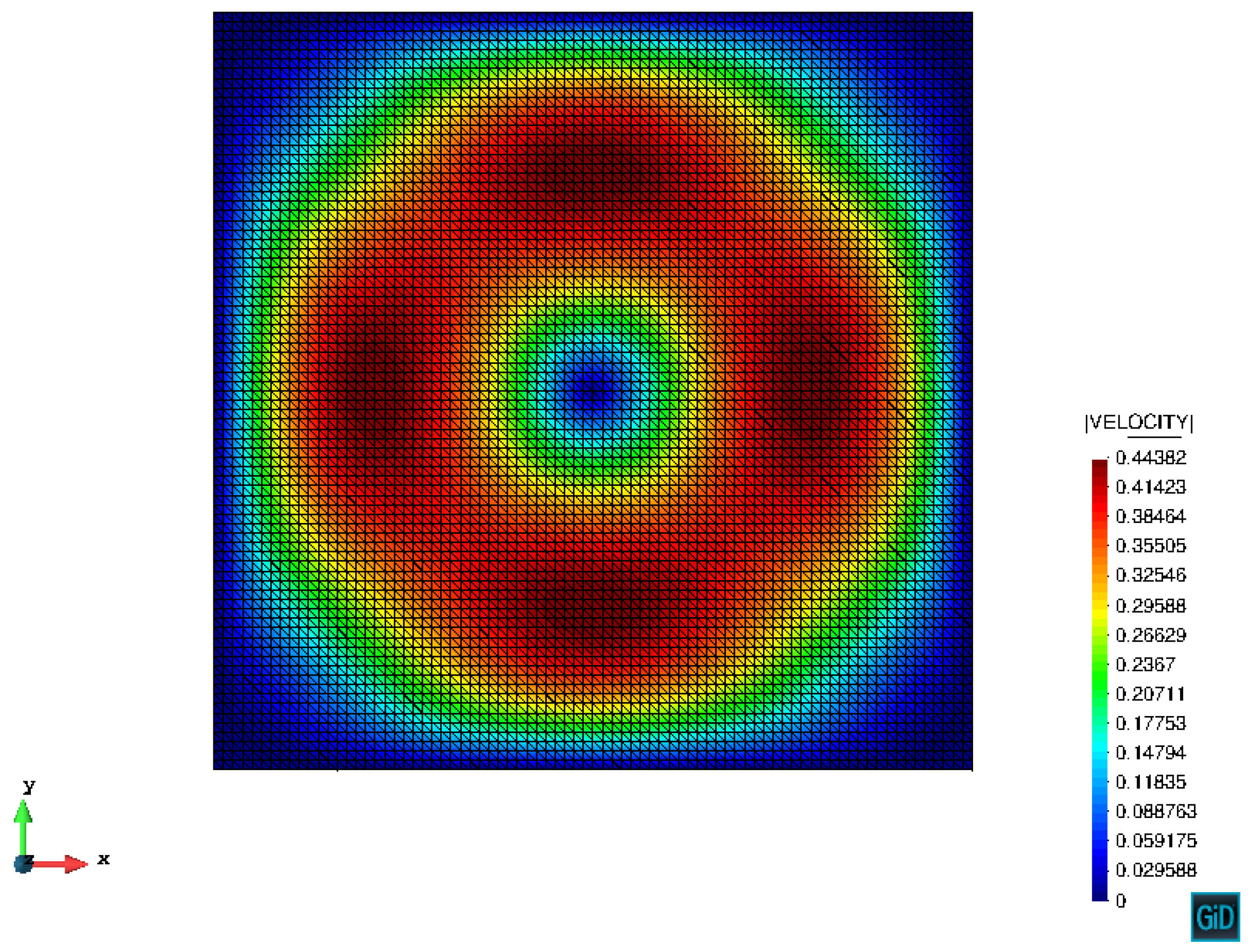
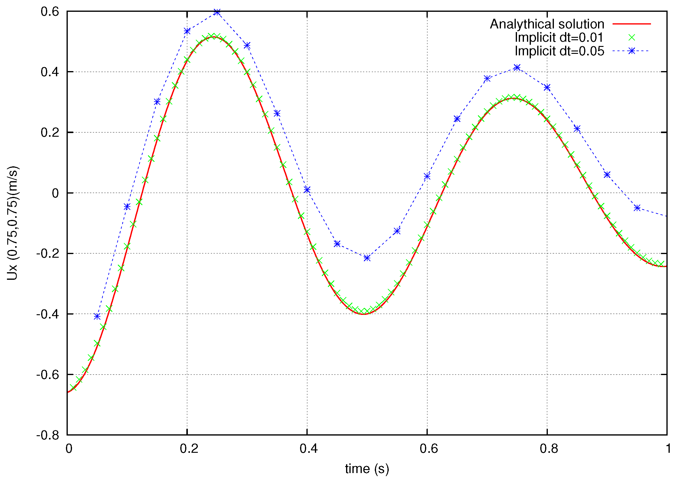
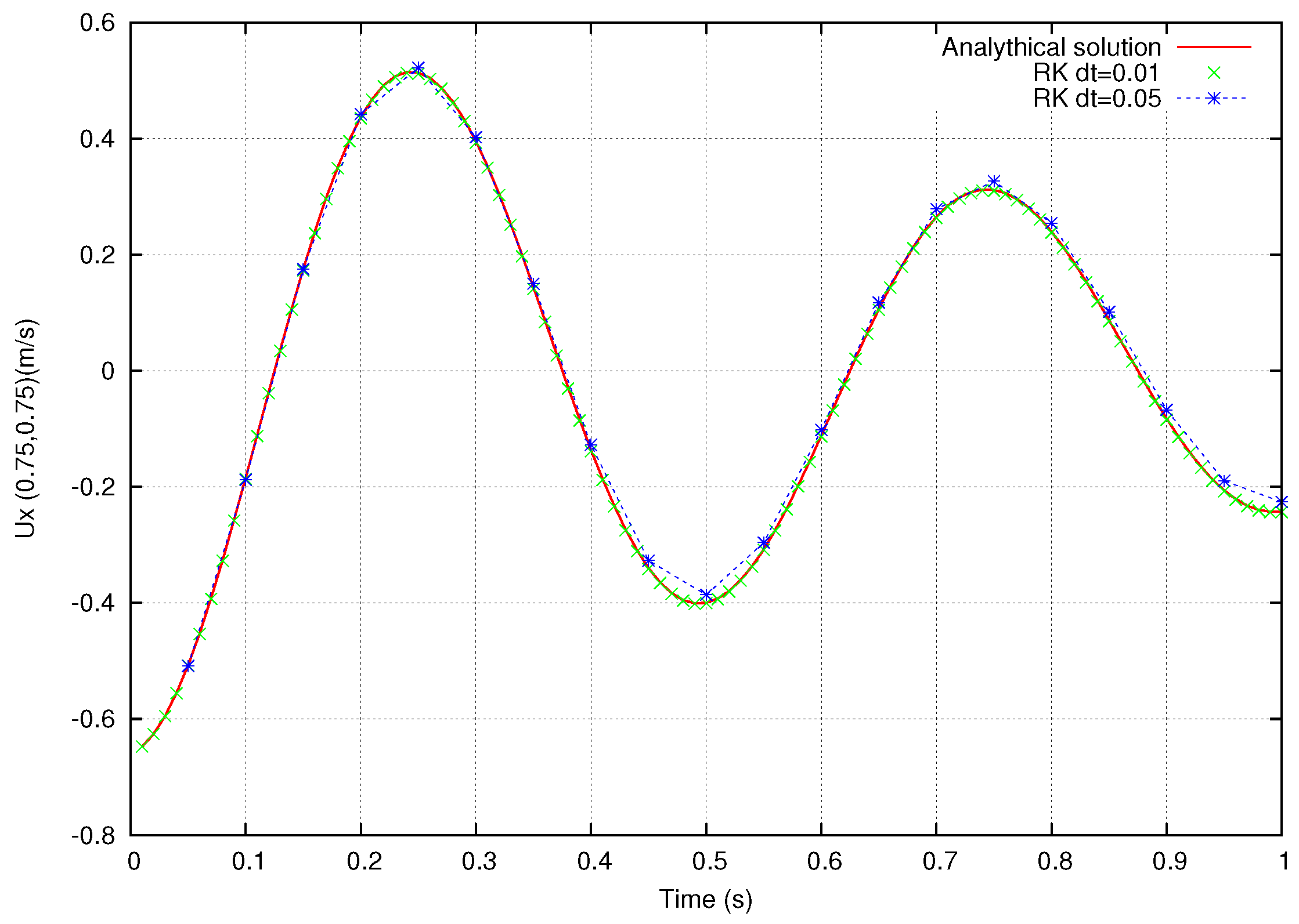
The velocity field at t = 1.0 is shown in Figure 1. The evolution of the horizontal velocity component $U_x$ at the point (x, y) = (0.75, 0.75) obtained using the implicit and the present semi-explicit scheme is shown in Figure 2 and Figure 3, respectively. One can see that as the time step diminishes, both the proposed method and the fractional step method tend to the exact solution. However, for the large time step, the implicit scheme clearly exhibits large error, while the semi-explicit Runge–Kutta scheme results in a solution nearly coinciding with the analytic one.

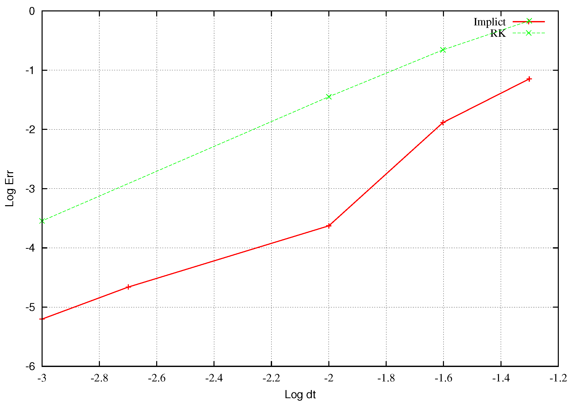
For assessing the accuracy quantitatively, the convergence of the time approximation is displayed in Figure 4. In order to obtain the graphs, the test was performed using various time step sizes in the range between $\Delta t$ = 0.05 s and $\Delta t$ = 0.001 s. Error versus time step size was plotted for the proposed semi-explicit and for the implicit method. The logarithmic scale was used. The error was computed as the sum of the nodal errors at time t = 1 s: $Err={\sum }_n\frac{|{\mathbf{u}}_{FE}-{\mathbf{u}}_{exact}|}{|{\mathbf{u}}_{exact}|}$ (n is the number of nodes).

One can see that both schemes exhibit quadratic convergence. However, the error introduced by the proposed method is considerably smaller than that of the implicit method for a given time step. For example, the semi-explicit Runge–Kutta scheme with $\Delta t$ = 0.01 leads to the same error as the implicit scheme with $\Delta t$ = 0.001. This indicates that provided s lower computational cost (per time step) of the semi-explicit scheme, a considerable gain in the overall computational time is expected.

3.2. Computational Efficiency of the Scheme

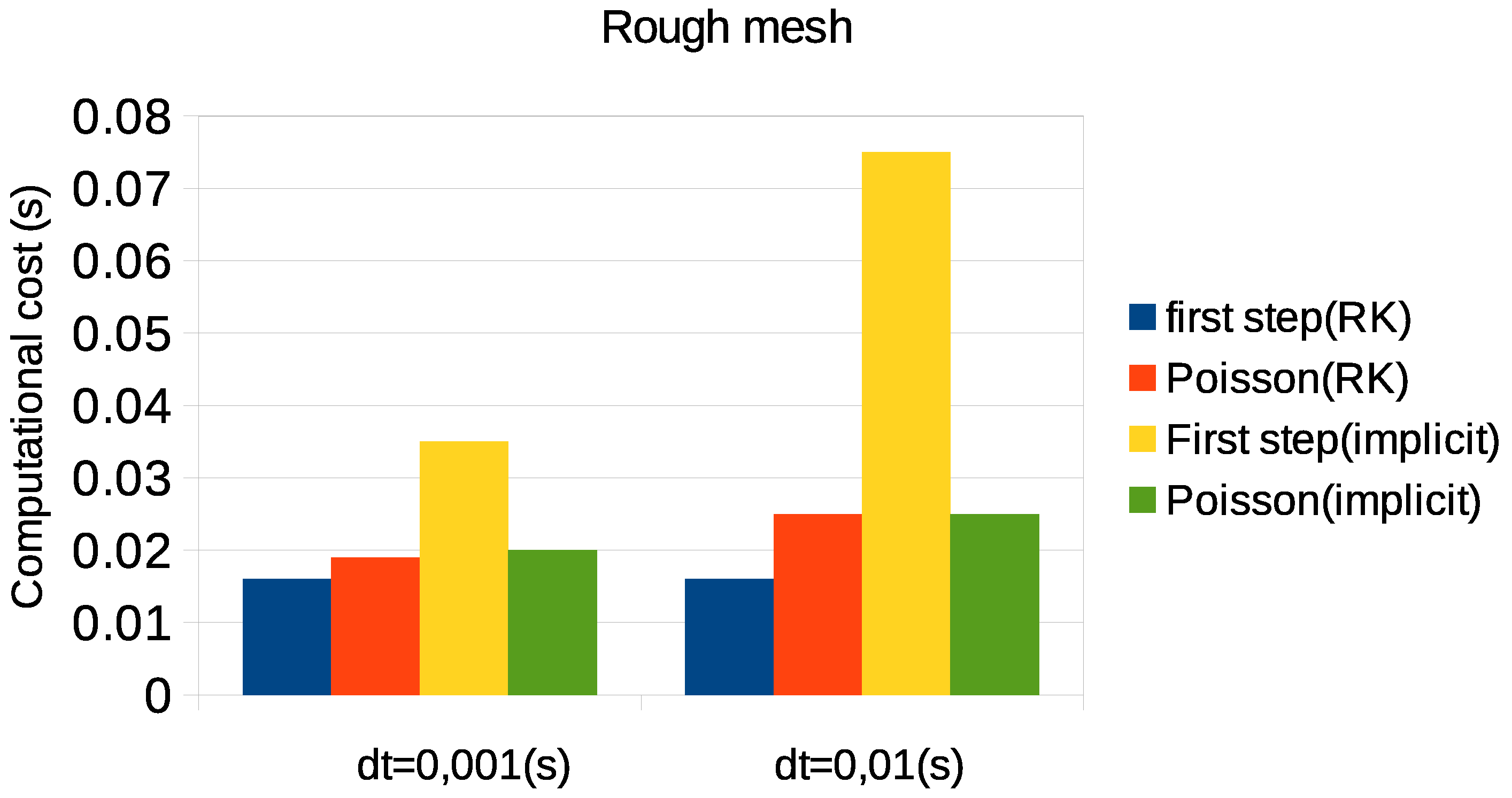
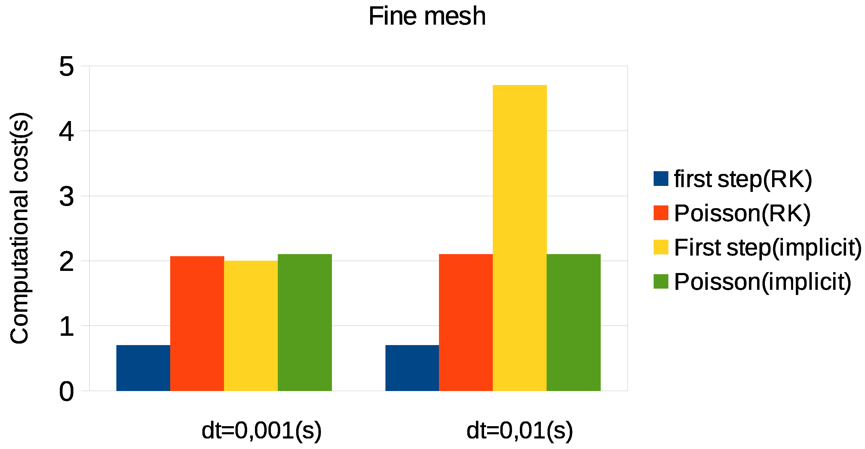
In order to highlight the computational efficiency properties of the proposed method, the test described in the previous sub-section was performed using two time step sizes ($\Delta t$ = 0.01 s and $\Delta t$ = 0.001 s) and two meshes (rough mesh: 6500 nodes and fine mesh: 160,000 nodes). The computational cost of different solution steps was estimated.

The test was performed on an Intel i5 desktop computer. It was executed on a single thread in order to gain the insight of the efficiency of the scheme without considering the gains obtained by parallel implementation. Poisson’s equation was solved using the biconjugate gradient stabilized algorithm with a diagonal preconditioning and a fixed tolerance of ${10}^{-3}$.

The computational times corresponding to the solution of the fractional momentum equation (first step) and the pressure Poisson equation are displayed. The computational cost of the momentum equation correction is not displayed, being negligible. Computational times were calculated as the average over all time steps.

Figure 5 shows the computational times corresponding to the tests performed on the rough mesh. One can see that the costs of the solution of Poisson’s equation using both the proposed and the implicit schemes are nearly identical (around 0.02 s) for all considered time step sizes. The computational cost of the momentum equation solution equals 0.015 s in the case of the semi-explicit scheme and 0.035 s in the case of the implicit scheme for $\Delta t$ = 0.001 s. Increasing the time step to 0.01 s, the computational cost of the first step nearly does not change for the semi-explicit scheme, while it increases to 0.075 s in the case of the implicit scheme. This occurs due to the increased number of non-linear iterations necessary for the convergence of the implicit scheme.

Figure 6 shows the computational times obtained in the simulation carried out on a fine mesh. Similar to the results shown in the previous figure, the time required for the solution of Poisson’s equation is similar in both methods, while there is a considerable difference in the time required for the solution of the fractional momentum equation (first step). One can see again that for larger time steps, several non-linear iterations are required in the case of the implicit scheme. In the considered case, for $\Delta t$ = 0.01 s, the overall computational cost of the implicit method is more than three-times larger than that of the semi-explicit scheme (the cost of the first step is more than five-times higher in the case of using the implicit scheme). We also note that Figure 4 indicates that for achieving a given accuracy, the semi-explicit scheme allows using much larger time steps. For instance, a relative error of approximately ${10}^{-4}$ requires using $\Delta t<$ 0.001 s in the case of the implicit scheme, while the semi-explicit scheme leads to this accuracy already for $\Delta t$ = 0.01 s. Thus, the overall computational cost corresponding to the time accuracy is much smaller in the case of using the semi-explicit scheme.

We note that the one can estimate the restrictions of the semi-explicit scheme for a given problem knowing Courant and Fourier numbers. The latter strongly restricts the time step in the case of high viscosities. However, such engineering fluids as air or water are characterized by low viscosity. Thus, the present methodology can be successfully used for a wide range of practical applications.

4. Summary and Conclusions

This paper has shown how an efficient semi-explicit strategy can be derived in the framework of the stabilized Galerkin finite element methods. A methodology based on a combination of the Runge–Kutta time integration scheme with the fractional step technique was presented. It was shown that introducing an approximation for the pressure at the intermediate steps of the Runge–Kutta method leads to a scheme where the implicit step necessary for computing the pressure is performed only once.

A priori estimates, as well as numerical tests have shown that the time accuracy of the resulting scheme reduces to the second order; however, the value of the error for a given time step is several orders of magnitude smaller than the one arising when applying fractional step to second-order implicit schemes. Thus, for the problems where critical time step estimates due to CFL (Courant-Friedrichs-Lewy) criteria are favorable, the method proposed here defines a very advantageous option in comparison with the implicit schemes.

The overall computational cost of the resulting method is governed by the cost of a single solution of the pressure Poisson equation, which is an equation of inhomogeneous Laplace type. Thus, an important step to make the proposed method even more efficient is to devise a scheme for minimizing the cost of solving Poisson’s equation, which can be done at the level of the linear solver following algebraic multi-grid or deflation techniques [32].

Another observation is that even though implicit time integration schemes are preferred in the literature against explicit ones, the latter are in a better position attending to the present hardware technology. This is oriented toward the usage of parallel computers and general purpose graphic processor units (GPGPU) [33]. Thus, the cost associated with the first part may be considerable reduced.

References

- Chorin, A. A numerical method for solving incompressible viscous problems. J. Comput. Phys. 1967, 2, 12–26. [Google Scholar] [CrossRef]
- Temam, R.M. Sur l’approximation de la solution des equations de Navier-Stokes par la methode des pase fractionaires. Arch. Ration. Mech. Anal. 1969, 32, 135–153. [Google Scholar] [CrossRef]
- Yanenko, N. The method of fractional steps for solving multidimensional problems of mathematical physics. Novosib. Sci. 1967, 196. [Google Scholar]
- Yanenko, N. The Method of Fractional Steps. The Solution of Problems of Mathematical Physics in Several Variables; Translated from Russian by Cheron, T.; Springer: Berlin/Heidelberg, Germany, 1971. [Google Scholar]
- Blair Perot, J. An analysis of the fractional step method. J. Comput. Phys. 1993, 108, 51–58. [Google Scholar] [CrossRef]
- Kim, J.; Moin, P. Application of a fractional-step method to incompressible Navier-Stokes equations. J. Comput. Phys. 1985, 59, 308–323. [Google Scholar] [CrossRef]
- Donea, J.; Giuliani, S.; Laval, H.; Quartapelle, L. Finite element solution of the unsteady Navier-Stokes equations by a fractional step method. Comput. Methods Appl. Mech. Eng. 1982, 30, 53–73. [Google Scholar] [CrossRef]
- Turek, S. A Comparative Study of Some Time-Stepping Techniques for the Incompressible Navier-Stokes Equations: From Fully Implicit Nonlinear Schemes to Semi-Implicit Projection Methods; IWR: Wroclaw, Poland, 1995. [Google Scholar]
- Strikwerda, J.; Lee, Y. The accuracy of the fractional step method. SIAM J. Numer. Anal. 1999, 37, 37–47. [Google Scholar] [CrossRef]
- Codina, R. Pressure stability in fractional step finite element method for incompressible flows. J. Comput. Phys. 2001, 170, 112–140. [Google Scholar] [CrossRef]
- Guermond, J.; Minev, P.; Shen, J. An Overview of Projection methods for incompressible flows. Comput. Methods Appl. Mech. Eng. 2006, 195, 6011–6045. [Google Scholar] [CrossRef]
- Könözsy, L.; Drikakis, D. A unified fractional-step, artificial compressibility and pressure-projection formulation for solving the incompressible Navier–Stokes equations. Commun. Computat. Phys. 2014, 16, 1135–1180. [Google Scholar]
- Codina, R.; Vázquez, M.; Zienkiewizc, O. A general algorithm for compressible and incompressible flows. Int. J. Numer. Methods Fluids 1998, 27, 13–32. [Google Scholar] [CrossRef]
- Ryzhakov, P.; Rossi, R.; Oñate, E. An algorithm for the simulation of thermally coupled low speed flow problems. Int. J. Numer. Methods Fluids 2012, 70, 1–19. [Google Scholar] [CrossRef]
- Ryzhakov, P.B.; Jarauta, A. An embedded approach for immiscible multi-fluid problems. Int. J. Numer. Methods Fluids 2016, 81, 357–376. [Google Scholar] [CrossRef]
- Ryzhakov, P.; Oñate, E.; Rossi, R.; Idelsohn, S.R. Improving mass conservation in simulation of incompressible flows. Int. J. Numer. Methods Eng. 2012, 90/12, 1435–1451. [Google Scholar] [CrossRef]
- Ryzhakov, P. A modified fractional step method for fluid—Structure interaction problems. Rev. Int. Métodos Numér. Cálc. Diseño Ing. 2017, 33, 58–64. [Google Scholar] [CrossRef]
- Nithiarasu, P. A matrix free fractional step method for static and dynamic incompressible solid mechanics. Int. J. Numer. Methods Eng. Sci. Mech. 2006, 7, 369–380. [Google Scholar] [CrossRef]
- Nikitin, N. Third-order-accurate semi-implicit Runge–Kutta scheme for incompressible Navier-Stokes equations. Int. J. Numer. Methods Fluids 2006, 51, 221–233. [Google Scholar] [CrossRef]
- Ascher, U.; Ruuth, S.; Spiteri, R. Implicit-explicit Runge-Kutta methods for time-dependent partial differential equations. Appl. Numer. Math. 1997, 25, 151–167. [Google Scholar] [CrossRef]
- Sanderse, B.; Koren, B. Accuracy analysis of explicit Runge–Kutta methods applied to the incompressible Navier–Stokes equations. J. Comput. Phys. 2012, 231, 3041–3063. [Google Scholar] [CrossRef]
- Fishpool, G.; Leschziner, M. Stability bounds for explicit fractional-step schemes for the Navier–Stokes equations at high Reynolds number. Comput. Fluids 2009, 38, 1289–1298. [Google Scholar] [CrossRef]
- Kampanis, N.A.; Ekaterinaris, J.A. A staggered grid, high-order accurate method for the incompressible Navier–Stokes equations. J. Comput. Phys. 2006, 215, 589–613. [Google Scholar] [CrossRef]
- Ha, S.; Park, J.; You, D. A GPU-accelerated semi-implicit fractional-step method for numerical solutions of incompressible Navier–Stokes equations. J. Comput. Phys. 2018, 352, 246–264. [Google Scholar] [CrossRef]
- Le, H.; Moin, P. An improvement of fractional step methods for the incompressible Navier–Stokes equations. J. Comput. Phys. 1991, 92, 369–379. [Google Scholar] [CrossRef]
- Pareschi, L.; Russo, G. Implicit-explicit Runge–Kutta schemes for stiff systems of differential equations. Recent Trends Numer. Anal. 2000, 3, 269–289. [Google Scholar]
- Bathe, K.J. The inf–sup condition and its evaluation for mixed finite element methods. Comput. Struct. 2001, 79, 243–252. [Google Scholar] [CrossRef]
- Donea, J.; Huerta, A. Finite Element Method for Flow Problems; Wiley: New York, NY, USA, 2003. [Google Scholar]
- Codina, R. A stabilized finite element method for generalized stationary incompressible flows. Comput. Methods Appl. Mech. Eng. 2001, 190, 2681–2706. [Google Scholar] [CrossRef]
- Dadvand, P.; Rossi, R.; Oñate, E. An object-oriented environment for developing finite element codes for multi-disciplinary applications. Arch. Comput. Methods Eng. 2010, 17/3, 253–297. [Google Scholar] [CrossRef]
- Ryzhakov, P.; Cotela, J.; Rossi, R.; Oñate, E. A two-step monolithic method for the efficient simulation of incompressible flows. Int. J. Numer. Methods Fluids 2014, 74, 919–934. [Google Scholar] [CrossRef]
- Brandt, A.; Livne, O. Multigrid Techniques: 1984 Guide with Applications to Fluid Dynamics, Revised Edition; SIAM: Philadelphia, PA, USA, 2011. [Google Scholar]
- Griebel, M.; Zaspel, P. A multi-GPU accelerated solver for the three-dimensional two-phase incompressible Navier-Stokes equations. Comput. Sci. Res. Dev. 2010, 25, 65–73. [Google Scholar] [CrossRef]
Figure 1.
Computational mesh and velocity field at t = 1 s. Solution obtained using the semi-explicit Runge–Kutta scheme.
Figure 2.
Temporal evolution of the horizontal velocity at (x, y) = (0.75, 0.75). Implicit second order backward differentiation formula (BDF2) scheme.
Figure 3.
Temporal evolution of the horizontal velocity at (x, y) = (0.75, 0.75). Semi-explicit Runge–Kutta scheme.
Figure 4.
Error at t = 1 s against the time step, logarithmic scale.
Figure 5.
Computational time of different solution steps. Semi-explicit vs. implicit method. Mesh of 6500 nodes.
Figure 6.
Computational time of different solution steps. Semi-explicit vs. implicit method. Mesh of 160,000 nodes.
© 2018 by the authors. Licensee MDPI, Basel, Switzerland. This article is an open access article distributed under the terms and conditions of the Creative Commons Attribution (CC BY) license (http://creativecommons.org/licenses/by/4.0/).
Share and Cite
MDPI and ACS Style
Ryzhakov, P.; Marti, J. A Semi-Explicit Multi-Step Method for Solving Incompressible Navier-Stokes Equations. Appl. Sci. 2018, 8, 119. https://doi.org/10.3390/app8010119
AMA Style
Ryzhakov P, Marti J. A Semi-Explicit Multi-Step Method for Solving Incompressible Navier-Stokes Equations. Applied Sciences. 2018; 8(1):119. https://doi.org/10.3390/app8010119
Chicago/Turabian StyleRyzhakov, Pavel, and Julio Marti. 2018. "A Semi-Explicit Multi-Step Method for Solving Incompressible Navier-Stokes Equations" Applied Sciences 8, no. 1: 119. https://doi.org/10.3390/app8010119
Note that from the first issue of 2016, this journal uses article numbers instead of page numbers. See further details here.