The NARX Model-Based System Identification on Nonlinear, Rotor-Bearing Systems


1
School of Mechanical Engineering & Automation, Northeastern University, Shenyang 110819, China
2
Key Laboratory of Vibration and Control of Aero-Propulsion System Ministry of Education, Northeastern University, Shenyang 110819, China
3
Department of Automatic Control and System Engineering, University of Sheffield, Sheffield S13JD, UK
*
Author to whom correspondence should be addressed.
Appl. Sci. 2017, 7(9), 911; https://doi.org/10.3390/app7090911
Submission received: 19 July 2017
/
Revised: 11 August 2017
/
Accepted: 26 August 2017
/
Published: 5 September 2017
(This article belongs to the Section Mechanical Engineering)
Abstract
:In practice, it is usually difficult to obtain the physical model of nonlinear, rotor-bearing systems due to uncertain nonlinearities. In order to solve this issue to conduct the analysis and design of nonlinear, rotor-bearing systems, in this study, a data driven NARX (Nonlinear Auto-Regressive with exogenous inputs) model is identified. Due to the lack of the random input signal which is required in the identification of a system′s NARX model, for nonlinear, rotor-bearing systems, a new multi-harmonic input based model identification approach is introduced. Moreover, the identification results of NARX models on the nonlinear, rotor-bearing systems are validated under different conditions (such as: low speed, critical speed, and over critical speed), illustrating the applicability of the proposed approach. Finally, an experimental test is conducted to identify the NARX model of the nonlinear rotor test rig, showing that the NARX model can be used to reproduce the characteristics of the underlying system accurately, which provides a reliable model for dynamic analysis, control, and fault diagnosis of the nonlinear, rotor-bearing system.
1. Introduction
The rotor-bearing system is the main component of large-scale, rotatable equipment such as, e.g., aircraft engines and gas turbines, etc., and most of the rotor-bearing systems are significantly affected by nonlinearities [1]. In order to investigate the properties of nonlinear, rotor-bearing systems, mathematical models are important [2]. The mathematical models can generally be divided into two categories: the numerical model and the physical model [3]. For nonlinear, rotor-bearing systems, the systems are usually simplified into physical models based on mechanical or electrical-related theories [4,5]. For example, Hu et al. [6] established a 5 degree of freedom (5DOF) physical model about the aircraft engine spindle dual-rotor system. Zhou and Chen [7] introduced a dual rotor-ball and bearing-stator coupling dynamic system. However, those physical models are relatively simple to describe complex, nonlinear, rotor-bearing systems such as, e.g., large centrifugal compressors and steam turbines, etc., where strong nonlinearities have to be taken into account [8]. Moreover, in practice, it is also difficult to establish the physical model of a system due to its complexity and the lack of physical knowledge [9]. Fortunately, it is possible to build a data-driven model by using only input and output signals, which is widely applied in system analysis, design, and control for the advantages of efficiency and the capacity of tracking changes of the system [10].
In 1980s, the NARX (Nonlinear Auto-Regressive with Exogenous Inputs) model was introduced by Billings as a new representation for a wide class of discrete, nonlinear systems [11]. The Volterra series model [12], the block-structured model [13], and many neural network architectures [14] can all be considered as subsets of the NARX model [15]. In practice, many systems have been investigated by using the NARX model [16,17,18]. For example, Peng et al. [19] established a NARX model of aluminum plate with structure damage and then detected the location of damage by frequency domain analysis, which provided a theoretical support for structural damage detection in practical engineering. Besides, the NARX model can also be used in other industrial scenarios such as modeling the large horizontal axis wind turbine [20] and large horizontal lathes [21]. Considering the nonlinear, rotor-bearing system, Tang et al. [22] established a Volterra series model by using date sets of the vibration response under different positions; based on this model, the fault modes were identified. Jiang et al. [23] developed the Volterra series model to detect the crack of the two discs in the rotor-bearing system.
In general, a random signal is selected as the system input in the traditional NARX modeling process. This is because the random signal contains different frequency and amplitude characteristics, and by using this, different properties of the system can be tested when the knowledge about system parameters and model structures is absent [24]. However, in practice, it is impossible to produce random input excitations when identifying rotor-bearing systems [25]. To address the aforementioned issue, in this study, a multi-harmonic signal generated by a speed-up process is applied as the system input to establish the NARX model. Moreover, a new approach to determine the NARX model by using the speed-up harmonic signal is introduced. Many researchers have analyzed the rotor-bearing system based on the speed-up process. For example, Li et al. [26] and Zhu et al. [27] extracted fault features of the rotor-bearing system by using the speed-up process, based on which the fault modes were identified. In this paper, the approach of identifying the NARX model of the nonlinear, rotor-bearing system is proposed by using the speed-up harmonic signal. The accuracy of the identified model is validated by using both numerical and experimental methods, and the results indicate that the NARX model of the nonlinear, rotor-bearing system can be used to represent different system characteristics, which contribute to the analysis, design, and fault diagnosis of the rotor-bearing system.
This paper is organized as follows. In Section 2, a typical nonlinear, rotor-bearing system is established and the inherent characteristics of the system are revealed. Section 3 introduces a new approach of identifying the NARX model of nonlinear systems based on a multi-harmonic input, which is discussed under different working conditions (such as: low speed, critical speed, and over critical speed). The NARX model is evaluated by two different validation methods and an error criterion. An experimental validation is discussed in Section 4, in which a test rig connected with the Labview test system and two eddy current displacement sensors are used. Finally, the three main conclusions are presented in Section 5, which provide an efficient method for numerical modeling of nonlinear, rotor-bearing system.
2. Nonlinear, Rotor-Bearing System Structure
2.1. System Structure
Considering the nonlinear contact force, the rotor-bearing system, placed horizontally with an unbalanced disc, is simplified (as the rotor is rigid) and supported by two symmetrical rolling bearings with the same parameters.
A simplified dynamic model of the rotor system is shown in Figure 1a, while the schematic of the rolling bearing is shown in Figure 1b. In Figure 1a, x-axis is the horizontal direction, and y-axis is the vertical direction; and in Figure 1b, and are the diameters of the outer race and inner race, respectively, and is the angle location of the ith ball.
The dynamic differential equation of the rotor-bearing system in Figure 1 can be defined as:
where is the equivalent mass of the rotor and the inner race at the disc; is the damping coefficient of the rotor at the disc and rolling bearing; is the rotor angular velocity; is the sum of the radial external force and the gravity of the rotor; is the rotor eccentricity distance; and are the supporting force components in the x and y directions, respectively. According to Hertzian contact theory, the forces generated from the rolling bearing are defined as [28]:
where represents the Hertzian contact stiffness; is the rolling bearing radial clearance; and is the contact deformation between the ith ball and the races. Also, the ith ball angle location is:
where is the number of balls of the rolling bearing.
2.2. System Inherent Characteristics
In system (1), given m = 1 kg, C = 200 Ns/m, = 7.055 × 10⁵ N/m, = 9, e = 2 mm, = 28.262 mm, = 18.783 mm, = 3 × 10⁻⁴ m. The first-order critical speed of the system can be obtained as = 320 rad/s, which is shown in Figure 2.
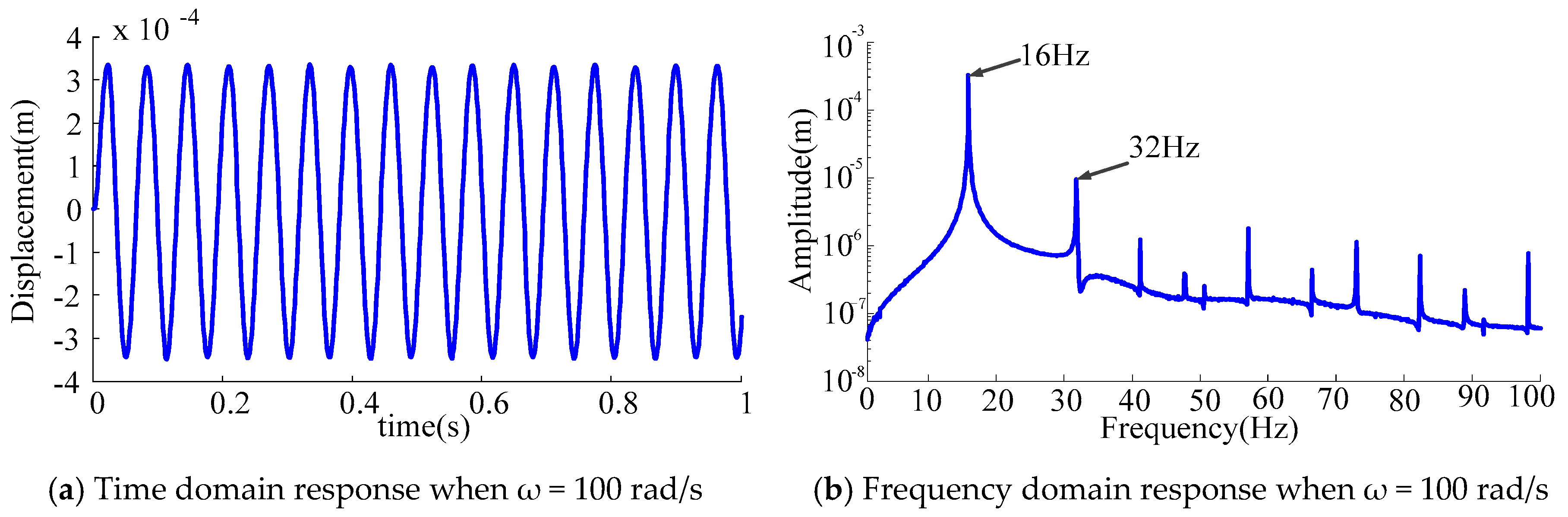
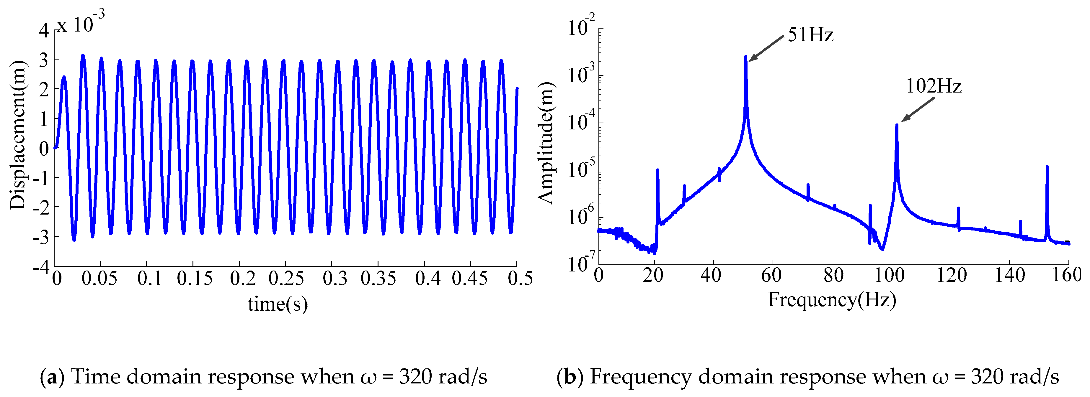
Three cases of the low speed ( = 100 rad/s), the critical speed ( = 320 rad/s), and the over critical speed ( = 500 rad/s) are discussed separately, as follows. The time domain and frequency domain responses of the rotor-bearing system are shown in Figure 3, Figure 4 and Figure 5, respectively.
As can be seen from Figure 3, Figure 4 and Figure 5, the second harmonics is the significant component under the three cases due to the effect of the nonlinear bearing force. Therefore, in the following section, the NARX model to the second order is identified based on the nonlinear, rotor-bearing system.
3. NARX Model on the Rotor-Bearing System
3.1. Identification of the NARX Model
A broad range of nonlinear systems can be described using NARX models, which can be expressed as [29]:
where is some nonlinear function, and are the maximum time lag for the system output and input, respectively, and and are the output and input sequence of the system, respectively.
The NARX model has several forms, among which the power polynomial representation is most commonly used in nonlinear system identification. Function in equation (4) is defined as the following polynomial expression:
where:
where are model coefficients; is the degree of polynomial nonlinearity; n = + .
Consider a generic linear-in-parameters representation of model (5) as:
where is the model coefficient of the mth term; is the number of all possible model terms, M = (n + l)!/(n!l!); is the regression which is formed by some combinations of the predetermined model variables, which are orderly chosen from the following vector .
The NARX model can be obtained by using FROLS (Forward Regression Orthogonal Least Squares) algorithm [30], which is a recursive algorithm based on ERR (Error Reduction Ratio) criterion to select significant model terms. The steps of FROLS are as follows:
● Step 1: Orthogonalization of model:
The NARX model (7) can be rewritten into a matrix form:
where is the regression matrix with the column vectors which consist of the values over the time history; is the number of sampling observations; is the coefficient vector.
Based on the Schmidt′s orthogonalization, the model (8) can be orthogonalized into [15]:
where is the orthogonalized matrix of is the corresponding coefficients vector, where:
● Step 2: Model term selection:
- A.
- Given , where the superscript (1) represents the first selecting step. can be calculated based on Equation (11).
Then obtain the column which has the largest ERR value:
where represents the value of the argument when the function reaches the maximum.
Given the corresponding term vector as the first model term vector of the orthogonalized matrix in (9), which means , and given .
- B.
- When the selection goes to step l, define , and based on the selected orthogonalized model term vectors , the lth model term vector is given as:
The ERR value of each vector and the one with maximum ERR value are obtained as:
Based on (16), one obtains the lth model term vector of the orthogonalized matrix in (9), which means , and given .
- C.
- The algorithm will stop selecting at the M’th step when the model structure satisfies the following condition:where is the threshold; M’ represents the total number of the selected model terms.
Based on (15)–(17), the M’th selected model term is given as .
The orthogonalized NARX model is given as:
● Step 3: Calculation of model coefficients:
As for model validation, there are two different methods, defined as OSA (One Step Ahead) and MPO (Model Predicted Output). It is difficult to give a general conclusion as to method should be used in a specific situation [32].
The concept of OSA validation can be explained by using a simple second-order NARX model:
Assume that a number of values if system input u(k) and y(k) are available. The OSA validation processes, starting from step 3, are then given as:
By comparison, the calculation of model output by the MPO method is completely different from the OSA method. Consider again the NARX model (21), for which the MPO can be defined as:
In this paper, the results are evaluated by time domain and spectrum graph, as well as RMSE (root mean square error (RMSE). The RMSE is given as:
where and are the predicted output and actual output, respectively; N is the number of sampling observations.
3.2. NARX Model Subjected to Multi-Harmonic Excitation
NARX approach is used in the system identification of the rotor-bearing system which is shown in Figure 1, where the system is subjected to unbalanced force in the horizontal direction. Considering the advantages of the speed-up process which have been discussed in the introduction, the multi-harmonic signal rad/s is defined as the system input excitation, and the output of the system is defined as the horizontal vibration response of the unbalanced disc.
The NARX model for the rotor-bearing system in Figure 1 is identified as:
The 15 selected model terms, ranked in order of significance, are shown in Table 1.
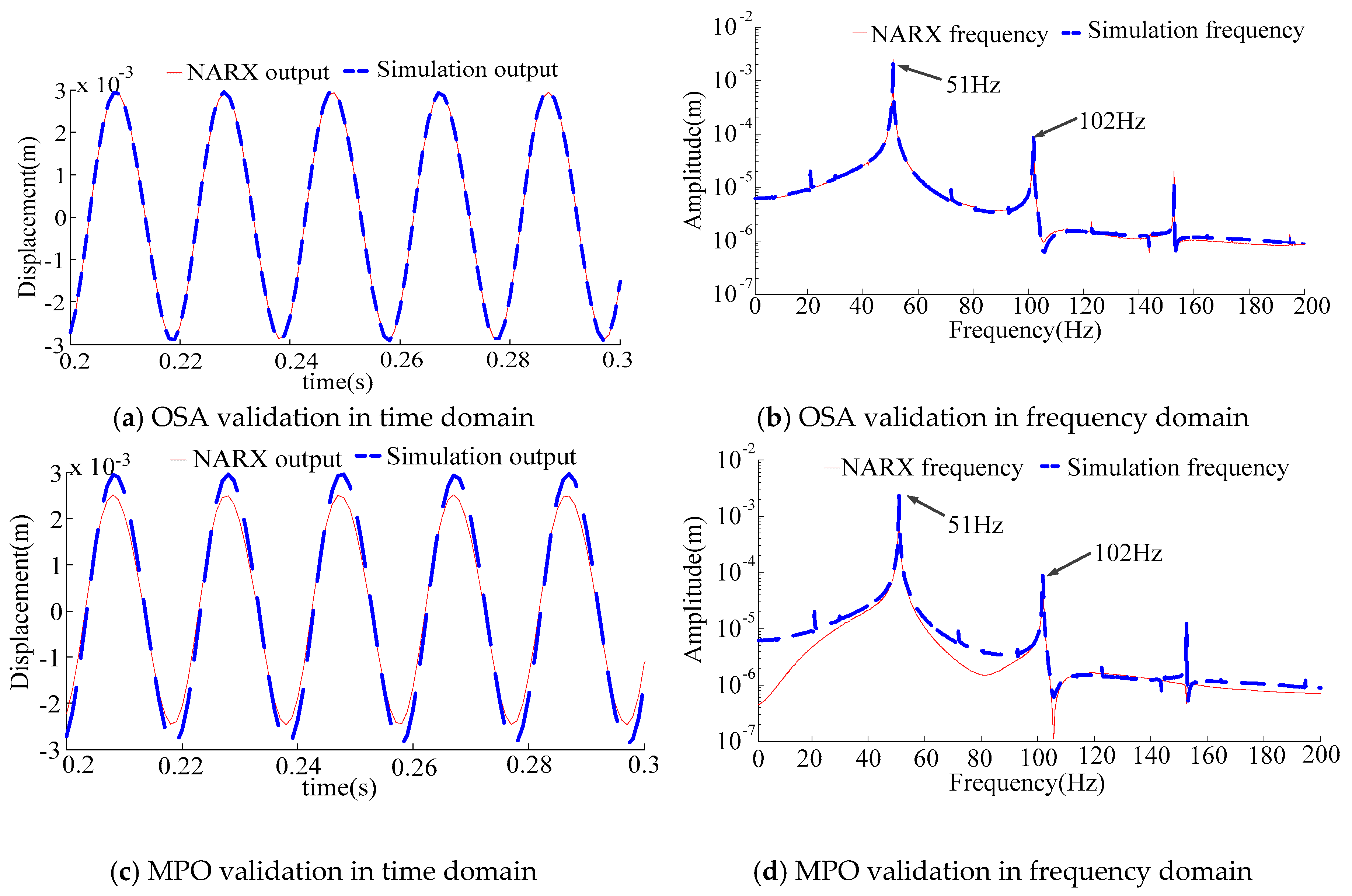
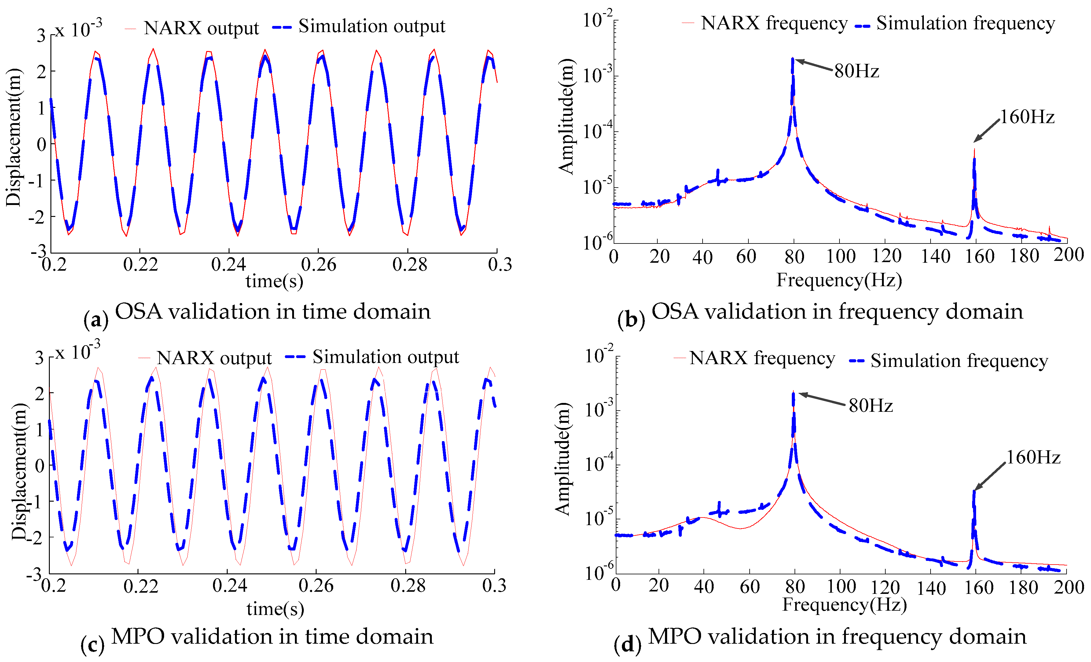
In the following study, the NARX model (25) is validated under the excitations of the low speed ( = 100 rad/s), the critical speed ( = 320 rad/s), and the over critical speed ( = 500 rad/s), respectively. The predicted output responses by the NARX model are compared with the simulation results in both the time and the frequency domain. Moreover, the OSA and the MPO methods are also discussed. The results are shown in Figure 6, Figure 7 and Figure 8. Also, the model is also evaluated by RMSE, which is shown in Table 2.
Figure 6, Figure 7 and Figure 8 and Table 2 indicate that the NARX model over a wide frequency range can be accurately predicted by using the OSA method. However, by using the MPO method, the output predictions have significant errors over the whole frequency range. Therefore, in practice, the NARX model identified over a wide frequency range cannot be used to reproduce the structure of the nonlinear, rotor-bearing system.
To address this issue, in the following study, NARX models are separately identified under, a more narrow frequency range, such as the low frequency range, the natural frequency range, or the high frequency range, respectively.
3.3. NARX Model under Different Frequency Ranges
In this section, three different NARX models are separately established by using the speed-up input signal over different frequency ranges, and the results are validated by using the MPO method, which indicates that the NARX model of the rotor-bearing system covering a relatively narrow frequency range can reflect the system characteristic accurately.
3.3.1 Under the Low-Speed Condition
When the input signal contains the frequency of rad/s, the NARX model can be identified as:
where the harmonic input with = 100 rad/s is used to test the model in both the time and the frequency domain, shown in Figure 9. Also, the RMSE is 9.0925 × 10⁻⁷ m.
3.3.2 Under the Critical Speed Condition
When the input signal contains the frequency of rad/s, the NARX model can be identified as:
where the harmonic input with = 320 rad/s is used to test the model in both the time and the frequency domain, shown in Figure 10. Also, the RMES is 2.4703 × 10⁻⁶ m.
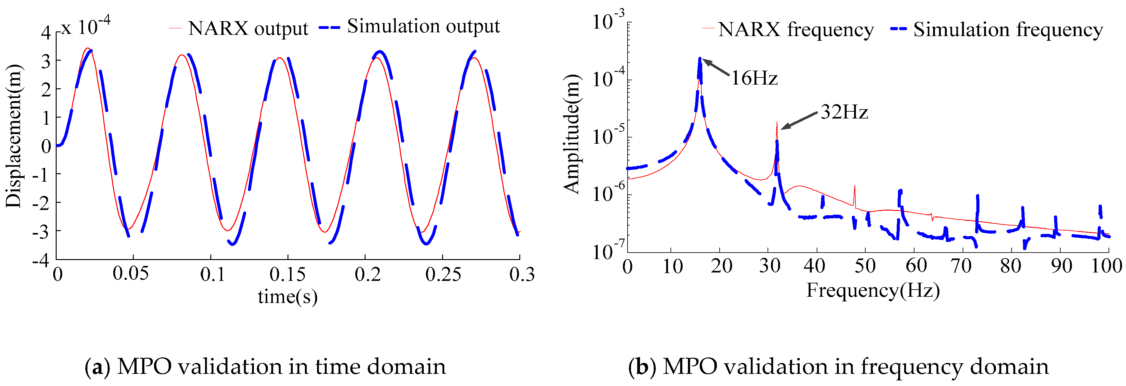
3.3.3. Under the Over-Critical Speed Condition
When the input signal contains the frequency of rad/s, the NARX model can be identified as:
where the harmonic input with = 500 rad/s is used to test the model in both the time and the frequency domain, presenting in Figure 11. And the RMES is 6.4411 × 10⁻⁶ m.
Figure 11 indicates that the NARX model identified in the low frequency range provides a more accurate prediction result than that of (25). Also, the RMSE is better than 1.4032 × 10⁻⁵ m, as shown in Table 2.
As the above three sections indicate, both the graphs and the values of RMSE show a better accuracy than that of Section 3.2. That is, from both a qualitative and quantitative point of view, the method of narrowing the frequency range of input excitations can optimize the NARX model and make the model perform better.
4. Experimental Verification
In order to validate the proposed identification method of the nonlinear, rotor-bearing system, a rotor test rig is taken for verification, where the eddy current displacement sensor is arranged to measure the response, and the added bolt is expected to reinforce unbalanced force, as shown in Figure 12a. The test rig is connected with the Labview test system, as shown in Figure 12b.
Concerned with safeness, the test rig, which has a critical speed of 229 rad/s, is operated under low speed case. Define the multi-harmonic rad/s as the system input excitation, and the output of the system is considered as the horizontal vibration response.
The NARX model of the rotor test rig is established with the test data of 84, 85, 86, 87, and 88 rad/s. Based on FROLS algorithm, a 3 order NARX model is identified as follow (Table 3):
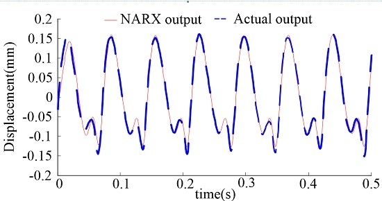
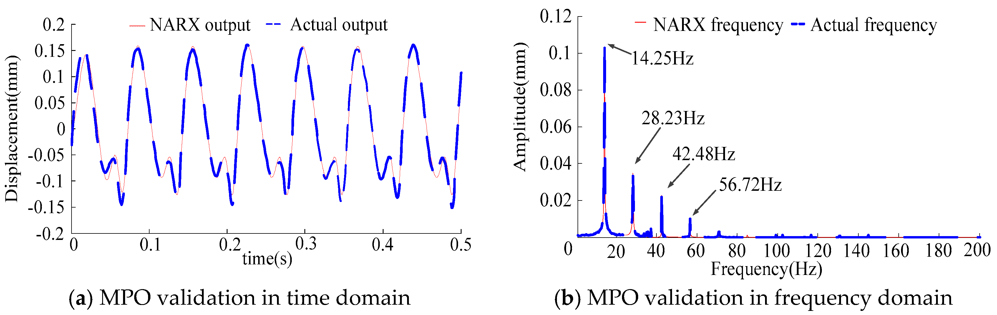
The input excitation = 89 rad/s is used to verify the identified NARX model in both the time and frequency domains by using the MPO method, and the results are shown in Figure 13. At the same time, the RMSE is calculated as 8.2272 × 10⁻⁶ m.
As Figure 13 implies, the NARX model shows satisfying accuracy. It indicates that the NARX model of the rotor test rig can predict the system output and reflect the system dynamic characteristics. Therefore, the NARX model provides a theoretical basis for analysis, design, and fault diagnosis of the nonlinear, rotor-bearing system.
5. Conclusions
- Mathematical models are important in the analysis, design, and fault diagnose of rotor-bearing systems. However, due to the complex structure and other factors, it is impossible to establish an accurate physical model. Thus, in this paper, an identification method of the nonlinear, rotor-bearing system based on NARX model is proposed.
- The experimental results indicate that the NARX model can reproduce the underlying nonlinear, rotor-bearing system accurately. Furthermore, the method enriches the nonlinear, rotor-bearing modeling theory and provides a reliable model for dynamic analysis, design, and fault diagnosis of the rotor-bearing system, which is of practical significance.
- The NARX model under multi-harmonic excitation can reflect a broad range of system characteristics. The MPO and OSA methods are used in model validation. The results indicate that it is inappropriate to use the OSA method when establishing the nonlinear, rotor-bearing system.
Acknowledgments
This work was supported by the National Science Foundation of China (grant numbers 11572082); the Fundamental Research Funds for the Central Universities of China (grant numbers N160312001, N150304004); and the Excellent Talents Support Program in Institutions of Higher Learning in Liaoning Province of China (grant numbers LJQ2015038).
Author Contributions
Ying Ma and Yunpeng Zhu conceived and designed the study; Ying Ma and Haopeng Liu performed the experiments; Ying Ma wrote the manuscript. Zhong Luo and Fei Wang reviewed and edited the manuscript. All authors read and approved the manuscript.
Conflicts of Interest
The founding sponsors had no role in the design of the study; in the collection, analyses, or interpretation of data; in the writing of the manuscript, and in the decision to publish the results.
References
- Rao, J.S. Rotor Dynamics; New Age International: Delhi, India, 1996. [Google Scholar]
- Xiang, L.; Hu, A.; Hou, L. Nonlinear coupled dynamics of an asymmetric double-disc rotor-bearing system under rub-impact and oil-film forces. J. Appl. Math. Model. 2016, 40, 4505–4523. [Google Scholar] [CrossRef]
- Nowak, R.D. Nonlinear system identification. J. Circuits Syst. Signal Process. 2002, 21, 109–122. [Google Scholar] [CrossRef]
- Fonseca, C.A.; Santos, I.F.; Weber, H.I. Influence of unbalance levels on nonlinear dynamics of a rotor-backup rolling bearing system. J. Sound Vib. 2017, 394, 482–496. [Google Scholar] [CrossRef]
- Luo, Z.; Chen, G.; Li, J. Design of Dynamic Similarity Model of Rotor System Considering the Bearing Stiffness. J. Northeast. Univ. Nat. Sci. 2015, 36, 402–405. [Google Scholar]
- Hu, Q.H.; Sier, D.; Hongfei, T.A. 5-DOF Model for Aeroengine Spindle Dual-Rotor System Analysis. Chin. J. Aeronaut. 2011, 24, 224–234. [Google Scholar] [CrossRef]
- Zhou, H.; Chen, G. Dynamic response analysis of dual rotor-ball bearing-stator coupling system for aero-engine. J. Aerosp. Power 2009, 24, 1284–1291. [Google Scholar]
- Ma, H.; Yu, T.; Han, Q. Time–frequency features of two types of coupled rub-impact faults in rotor systems. J. Sound Vib. 2009, 321, 1109–1128. [Google Scholar] [CrossRef]
- Zhang, Y.; Bang, C.W.; Qiao, L.L. Uncertain responses of rotor-stator systems with rubbing. J. JSME Int. J. Ser. C Mech. Syst. Mach. Elem. Manuf. 2003, 46, 150–154. [Google Scholar] [CrossRef]
- Billings, S.A. Identification of nonlinear systems—A survey. IEE Proc. D Control Theory Appl. 1980, 127, 272–285. [Google Scholar] [CrossRef]
- Leontaritis, I.J.; Billings, S.A. Input-output parametric models for non-linear systems part I: Deterministic non-linear systems. J. Int. J. Control 1985, 41, 303–328. [Google Scholar] [CrossRef]
- Xia, X.; Zhou, J.; Xiao, J. A novel identification method of Volterra series in rotor-bearing system for fault diagnosis. J. Mech. Syst. Signal Process. 2016, 66, 557–567. [Google Scholar] [CrossRef]
- Harnischmacher, G.; Marquardt, W. Nonlinear model predictive control of multivariable processes using block-structured models. J. Control Eng. Pract. 2007, 15, 1238–1256. [Google Scholar] [CrossRef]
- Arnaiz-González, Á.; Fernández-Valdivielso, A.; Bustillo, A. Using artificial neural networks for the prediction of dimensional error on inclined surfaces manufactured by ball-end milling. Int. J. Adv. Manuf. Technol. 2016, 83, 847–859. [Google Scholar]
- Billings, S.A. Nonlinear System Identification: NARMAX Methods in the Time, Frequency, and Spatio-Temporal Domains; John Wiley & Sons: Hoboken, NJ, USA, 2013. [Google Scholar]
- Cadenas, E.; Rivera, W.; Campos, A.R. Wind speed prediction using a univariate ARIMA model and a multivariate NARX model. J. Energies 2016, 9, 109. [Google Scholar] [CrossRef]
- Asgari, H.; Chen, X.Q.; Morini, M. NARX models for simulation of the start-up operation of a single-shaft gas turbine. J. Appl. Therm. Eng. 2016, 93, 368–376. [Google Scholar] [CrossRef]
- Ruano, A.E.; Fleming, P.J.; Teixeira, C. Nonlinear identification of aircraft gas-turbine dynamics. J. Neurocomput. 2003, 55, 551–579. [Google Scholar] [CrossRef]
- Peng, Z.K.; Lang, Z.Q.; Wolters, C. Feasibility study of structural damage detection using NARMAX modelling and Nonlinear Output Frequency Response Function based analysis. J. Mech. Syst. Signal Process. 2011, 25, 1045–1061. [Google Scholar] [CrossRef]
- Liu, X.; Lu, C.; Liang, S. Vibration-induced aerodynamic loads on large horizontal axis wind turbine blades. J. Appl. Energy 2017, 185, 1109–1119. [Google Scholar] [CrossRef]
- Urbikain, G.; Campa, F.J.; Zulaika, J.J. Preventing chatter vibrations in heavy-duty turning operations in large horizontal lathes. J. Sound Vib. 2015, 340, 317–330. [Google Scholar] [CrossRef]
- Tang, H.; Liao, Y.H.; Cao, J.Y. Fault diagnosis approach based on Volterra models. J. Mech. Syst. Signal Process. 2010, 24, 1099–1113. [Google Scholar] [CrossRef]
- Jing, J.; Li, Z.N.; Tang, G.S. Fault Diagnosis Method Based on Volterra Kernel Identification for Rotor Crack. J. Mach. Tool Hydraul. 2010, 23, 1001–3881. [Google Scholar]
- Lara, J.M.; Milani, B.E. Identification of neutralization process using multi-level pseudo-random signals. In Proceedings of the 2003 American Control Conference, Denver, CO, USA, 4–6 June 2003; pp. 3822–3827. [Google Scholar]
- Chen, S.; Billings, S.A.; Luo, W. Orthogonal least squares methods and their application to non-linear system identification. Int. J. Control 1989, 50, 1873–1896. [Google Scholar] [CrossRef]
- Li, Z.; He, Y.; Chu, F. Fault recognition method for speed-up and speed-down process of rotating machinery based on independent component analysis and Factorial Hidden Markov Model. J. Sound Vib. 2006, 291, 60–71. [Google Scholar] [CrossRef]
- Zhu, X.R.; Zhang, Y.Y.; Zhang, G.L. Fault Diagnosis for Speed-Up and Speed-Down Process of Rotor-Bearing System Based on Volterra Series Model and Neighborhood Rough Sets. J. Adv. Mater. Res. Trans. Tech. Publ. 2012, 411, 567–571. [Google Scholar] [CrossRef]
- Chen, G. Study on nonlinear dynamic response of an unbalanced rotor supported on ball bearing. J. Vib. Acoust. 2009, 131, 061001. [Google Scholar] [CrossRef]
- Wei, H.L.; Billings, S.A. Model structure selection using an integrated forward orthogonal search algorithm assisted by squared correlation and mutual information. Int. J. Model. Identif. Control 2008, 3, 341–356. [Google Scholar] [CrossRef]
- Billings, S.A.; Chen, S.; Korenberg, M.J. Identification of MIMO non-linear systems using a forward-regression orthogonal estimator. Int. J. Control 1989, 49, 2157–2189. [Google Scholar] [CrossRef]
- Wei, H.L.; Lang, Z.Q.; Billings, S.A. Constructing an overall dynamical model for a system with changing design parameter properties. Int. J. Model. Identif. Control 2008, 5, 93–104. [Google Scholar] [CrossRef]
- Ramírez, C.; Acuña, G. Forecasting cash demand in ATM using neural networks and least square support vector machine. J. Prog. Pattern Recognit. Image Anal. Comput. Vis. Appl. 2011, 7042, 515–522. [Google Scholar]
Figure 1.
Rotor-bearing dynamic model.
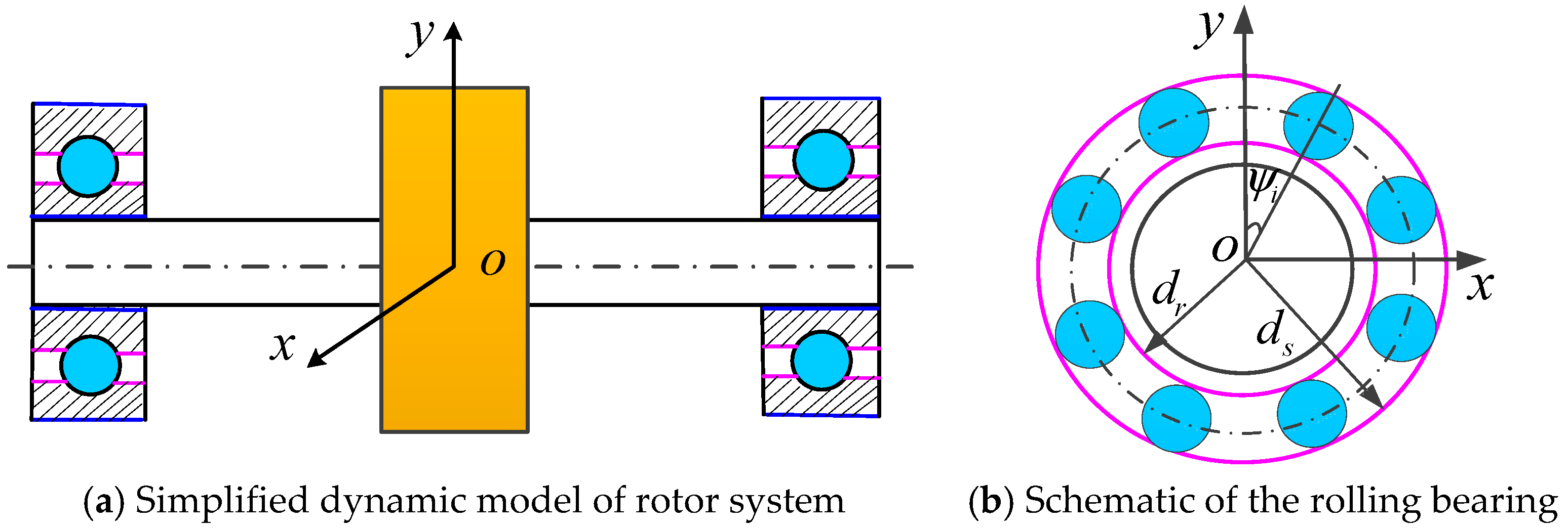
Figure 2.
Amplitude response curve of the system.
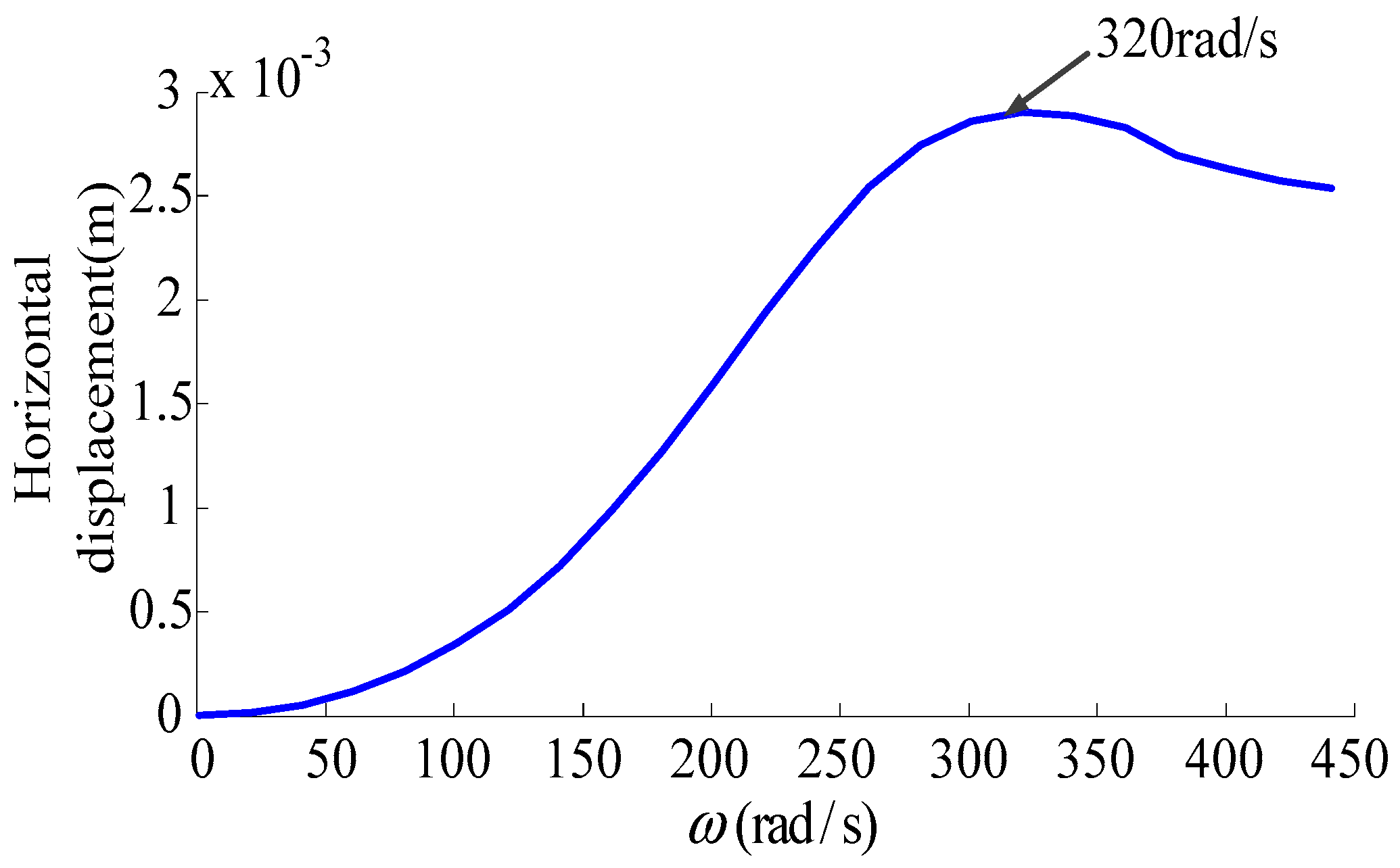
Figure 3.
Response of rotor-bearing system under low speed condition.

Figure 4.
Response of rotor-bearing system under critical speed condition.

Figure 5.
Response of rotor-bearing system under over critical speed condition.
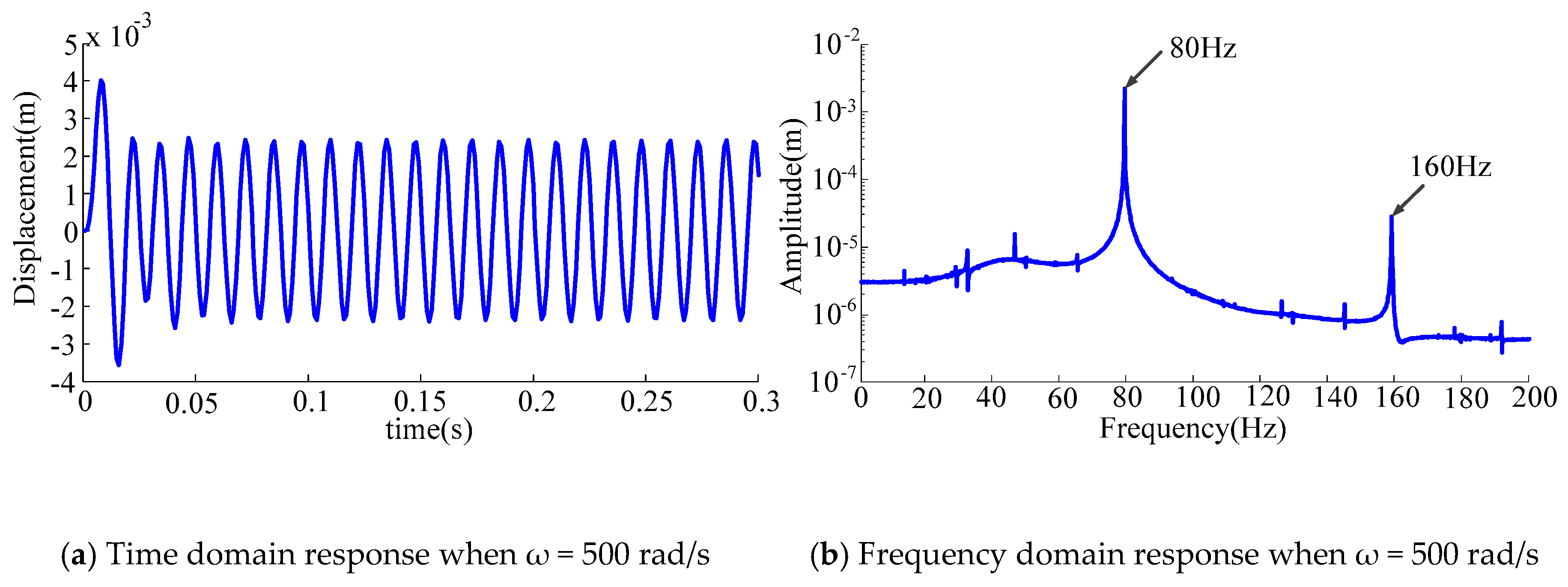
Figure 6.
Output comparison in time and frequency domain when = 100 rad/s.
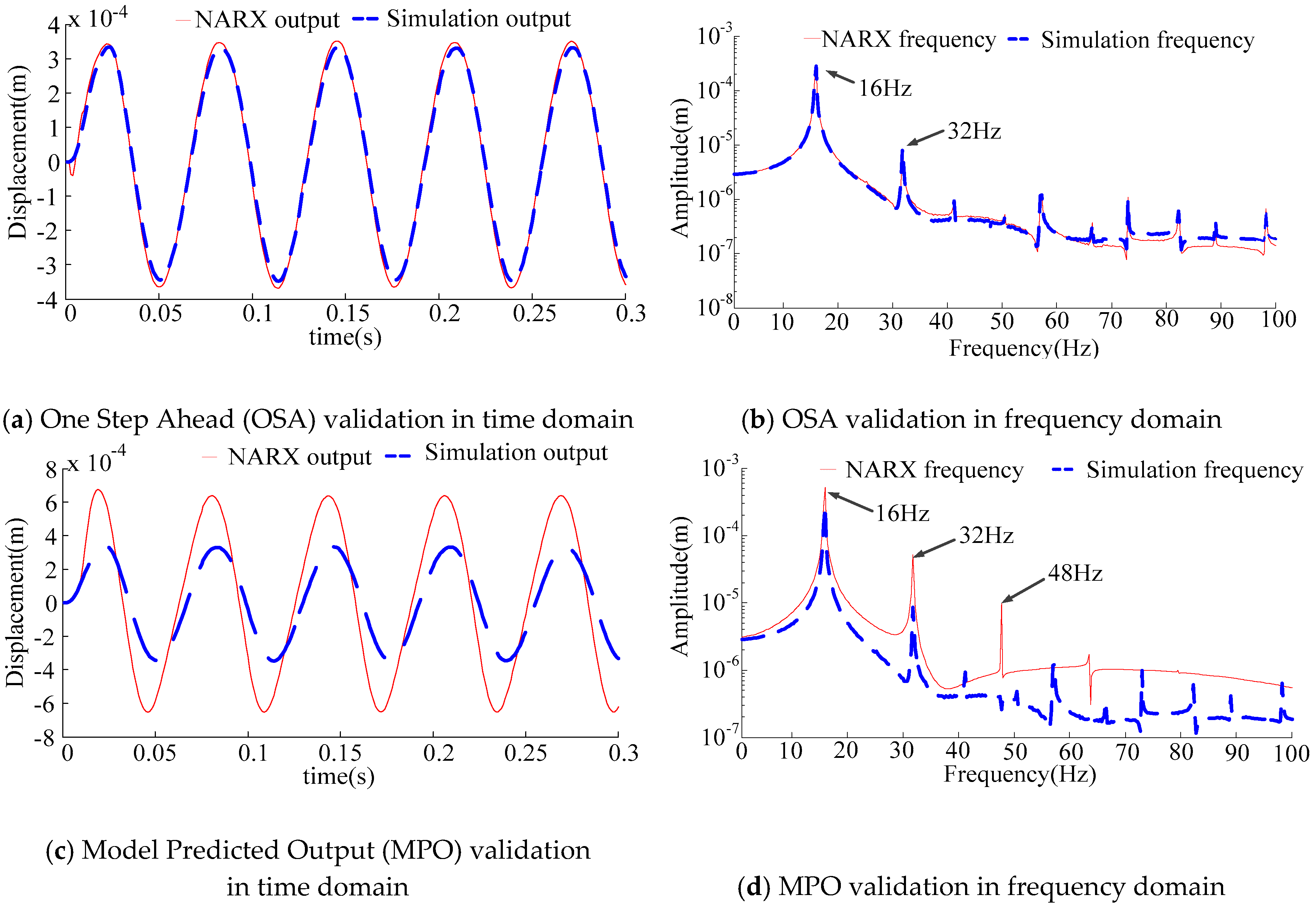
Figure 7.
Output comparison in time and frequency domain when = 320 rad/s.

Figure 8.
Output comparison in time and frequency domain when = 500 rad/s.

Figure 9.
Output comparison in time and frequency domain at a low speed.

Figure 10.
Output comparison in time and frequency domain at a critical speed.
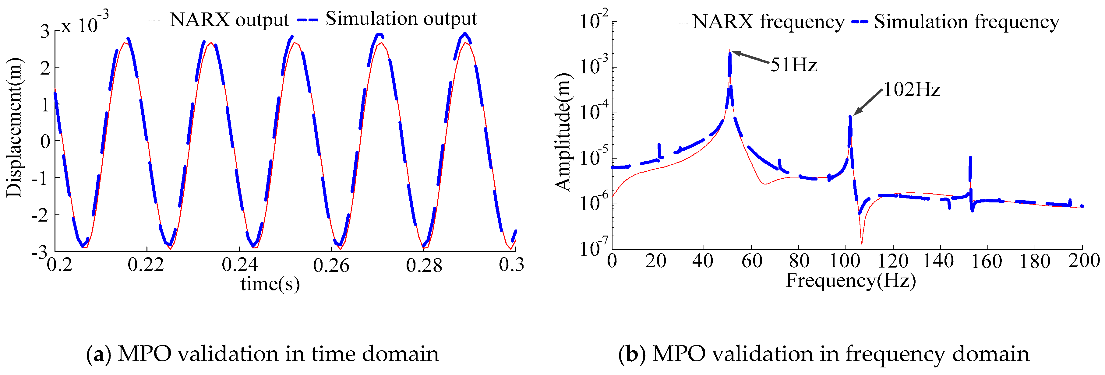
Figure 11.
Output comparison in time and frequency domain at an over critical speed.
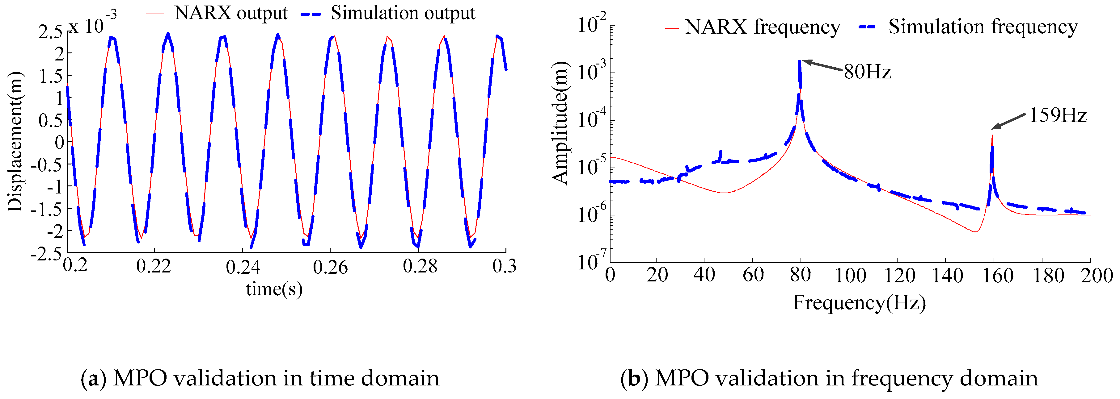
Figure 12.
Test set up.
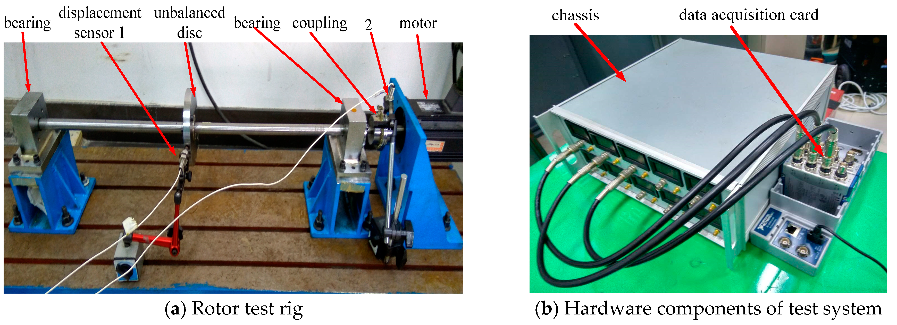
Figure 13.
Output comparison in time and frequency domain of the test.


Table 1.
Identification result of the example.
| Step | Term | Coefficient | ERR% |
|---|---|---|---|
| 1 | 1.5806 | 89.2521 | |
| 2 | −0.4635 | 10.3201 | |
| 3 | 2.9713 × 10⁻⁴ | 0.0963 | |
| 4 | 0.0931 | 0.0349 | |
| 5 | −2.2028 × 10⁻⁴ | 0.0227 | |
| 6 | −3.7178 × 10⁻⁴ | 0.0158 | |
| 7 | −5.3027 | 0.0119 | |
| 8 | −0.2637 | 0.0052 | |
| 9 | −0.0418 | 0.0078 | |
| 10 | 3.2374 × 10⁻⁴ | 0.0021 | |
| 11 | 1.8632 × 10⁻⁴ | 0.0023 | |
| 12 | −0.0091 | 0.0008 | |
| 13 | 0.0301 | 0.0009 | |
| 14 | −1.7955 × 10⁻⁴ | 0.0004 | |
| 15 | −8.0035 × 10⁻⁴ | 0.0004 | |
| Total | - | - | 99.7728 |
Table 2.
Root square mean error (RMSE) of MPO and OSA method in a large frequency range.
| Frequency Range (rad/s) | RMSE of MPO Method (m) | RMSE of OSA Method (m) |
|---|---|---|
| Low speed | 3.1582 × 10⁻⁶ | 2.9461 × 10⁻⁷ |
| Critical speed | 5.2704 × 10⁻⁶ | 4.7590 × 10⁻⁷ |
| Over critical speed | 1.4032 × 10⁻⁶ | 2.0754 × 10⁻⁶ |
Table 3.
Identification result of the test.
| Step | Term | Coefficient | ERR% |
|---|---|---|---|
| 1 | 1.8444 | 99.4393 | |
| 2 | −0.8595 | 0.5177 | |
| 3 | 0.1788 | 0.0027 | |
| 4 | −0.2439 | 0.0017 | |
| 5 | 0.0642 | 0.0138 | |
| 6 | 0.6580 | 0.0003 | |
| 7 | 0.1268 | 0.0006 | |
| 8 | −0.5515 | 0.0003 | |
| 9 | −0.0243 | 0.0003 | |
| 10 | −0.7159 | 0.0001 | |
| 11 | −0.1019 | 0.0001 | |
| 12 | 0.0250 | 0.0001 | |
| 13 | −0.0020 | 0.0001 | |
| 14 | 0.1688 | 0.0002 | |
| 15 | −0.1482 | 0.0005 | |
| Total | - | - | 99.9778 |
© 2017 by the authors. Licensee MDPI, Basel, Switzerland. This article is an open access article distributed under the terms and conditions of the Creative Commons Attribution (CC BY) license (http://creativecommons.org/licenses/by/4.0/).
Share and Cite
MDPI and ACS Style
Ma, Y.; Liu, H.; Zhu, Y.; Wang, F.; Luo, Z. The NARX Model-Based System Identification on Nonlinear, Rotor-Bearing Systems. Appl. Sci. 2017, 7, 911. https://doi.org/10.3390/app7090911
AMA Style
Ma Y, Liu H, Zhu Y, Wang F, Luo Z. The NARX Model-Based System Identification on Nonlinear, Rotor-Bearing Systems. Applied Sciences. 2017; 7(9):911. https://doi.org/10.3390/app7090911
Chicago/Turabian StyleMa, Ying, Haopeng Liu, Yunpeng Zhu, Fei Wang, and Zhong Luo. 2017. "The NARX Model-Based System Identification on Nonlinear, Rotor-Bearing Systems" Applied Sciences 7, no. 9: 911. https://doi.org/10.3390/app7090911
Note that from the first issue of 2016, this journal uses article numbers instead of page numbers. See further details here.