A Unified Approach for Reformulations of LRM/LRMM/LRRM Calibration Algorithms Based on the T-Matrix Representation

Abstract

This paper investigates a unified theory to derive vector network analyzer calibration algorithms based on the T-matrix representation, by which means the line-reflect-match (LRM), line-reflect-match-match (LRMM), and the line-reflect-reflect-match (LRRM) calibrations are formulated. The proposed calibration theory is more general than other versions of LRM, LRMM, and LRRM in that an arbitrary known two-port device can be used as the line standard L, rather than a perfect thru or transmission line. Experimental verifications of the proposed theory using on-wafer calibrations from 0.5 GHz to 110 GHz are given.

1. Introduction

The vector network analyzer (VNA) is the workhorse in most microwave laboratories, and its calibration technique has been well-developed through several decades [1]. As is well-known, the purpose of VNA calibration is to determine systematic errors to allow for the error correction of a device under test (DUT) measurement [2]. In general, the systematic errors, which are often lumped into error boxes and collectively called an error model, are described by scattering parameters (S-parameters) [3]. Based on the error model, the calibration algorithm can make use of some knowledge about the calibration standards to calculate the systematic errors, such as the classical SOLT calibration [3]. However, the S-parameter representation often obscures some simple and elegant mathematical solutions, although it permits an insight into the physical causes behind the transmission and reflection errors observed [4]. On the other hand, as an alternative representation of an error model, the scattering transfer parameters (T-parameters [5], also called cascade parameters [6]), which allow for the cascading of the matrix descriptions of the error boxes and the DUT, are typically used for deriving the thru-reflect-line (TRL), line-reflect-match (LRM, also often called thru-reflect-match (TRM)), and short-open-load-reciprocal (SOLR) algorithms, etc. [7,8,9,10,11]. The T-matrix form of error boxes can be utilized to establish the direct mapping of the waves at the ports of the DUT and the detected waves, but a perfect thru is often required to simplify the derivation of the calibration algorithms. In recent years, ABCD parameters have been used to reformulate calibration algorithms, because the impedance information about single-port standards is formulated easily [12,13,14]. Besides, ABCD parameters have the same advantage as T-parameters in that they allow matrix cascading.

Since the introduction of microwave probing, self-calibration techniques with fewer standards have progressed to achieve higher accuracy and more versatility. Around the late 1980s, the LRM calibration was proposed and has developed until present. The original LRM used a pair of fully known and symmetrical loads as the match standards M [8]. As a particular case of the Lxx calibration family studied in [15,16], the LRM technique exploited redundancy to determine the reflection coefficient of symmetrical reflection standards R, and then calculated all the seven error terms. However, the match standards M may be frequency dependent and non-identical in practice [17], so the LRM calibration has been constantly improved. Some examples of improvement in the literature are Ref. [14], which uses non-ideal match standards, and the line-reflect-match-match (LRMM) algorithm, which uses non-symmetrical load standards [14,18]. Meanwhile, the line-reflect-reflect-match (LRRM) calibration technique was proposed as an improvement to LRM. The advantage of LRRM is that only one partially known match standard is required [9,12,19]. Although the present LRM/LRMM/LRRM techniques are relatively mature, there is still a lack of a general theory which generalizes these three calibration algorithms.

A theory to formulate the SOLT and SOT-Line algorithms has been proposed in our early work [20]. The idea is originally from the principle of coordinate transformation, which regards the T-matrix of an error box as the transformation matrix in mathematics. Based on this idea, the T-matrix of an error box is defined to transform the waves at the test port to the detected waves. Meanwhile, two characteristic variables, which are essentially the ratios of the wave parameters, are newly introduced into the derivation of the algorithm. The de-embedding formulas are finally derived to obtain the corrected DUT parameters. However, the previous work is based on the 10-term error model, and is thus inapplicable for most self-calibration techniques [1]. In addition, the T-matrices of error boxes are not calculated.

This work further develops the previous theory, and the developed theory applies to LRM/LRMM/LRRM calibrations. This theory constructs the T-matrices of error boxes by using single-port measurements, and newly introduces three wave ratios to express the error boxes in the algorithm. Existing calibration methods, e.g., LRRM [12], also allow the reduction of calibration unknowns to three by utilizing a two-port standard measurement, but consequently a perfect thru or a known transmission line is often required for the convenience of analytical derivation [21,22]. In this theory, a unified mathematical framework is developed for LRM/LRMM/LRRM calibrations, and the line standard L can be an arbitrary known two-port standard. Although the early work [23] can also use the arbitrary known two-port standard, the formulas for the LRRM calibration were not described in sufficient detail. As will be shown in this paper, by using the proposed theory, LRM, LRMM, and LRRM calibration algorithms can be simply derived.

This paper is organized as follows. Section 2 explains the new general calibration theory. Section 3 gives the analytical derivations of the LRM/LRMM/LRRM calibration techniques using the new theory. In Section 4, the proposed theory is validated by experimental results. Some conclusions are drawn in Section 5.

2. Theory

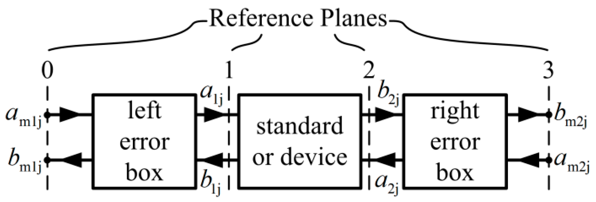
Error correction for two-port S-parameter measurements using a VNA is usually modeled as shown in Figure 1, where the waves a_ij and b_ij at the DUT are mapped to the raw measured waves a_mij and b_mij through the error boxes. The subscript ij (i, j = 1, 2) indicates that the parameter is located at port i and the power source is connected to port j. In this work, the crosstalk and switch terms are assumed to be negligible or have been accounted for. That is, VNA calibrations apply switch corrections independently and ignore (or pre-correct) crosstalk, resulting in the error model shown in Figure 1 [24,25].

In this work, the error boxes are represented in the form of T-matrices as follows:

$$\left[\begin{array}{c}{a}_{1\mathrm{j}}\\ b_{1\mathrm{j}}\end{array}\right]=[T_{10}]\left[\begin{array}{c}{a}_{\mathrm{m}1\mathrm{j}}\\ b_{\mathrm{m}1\mathrm{j}}\end{array}\right]$$

(1)

$$\left[\begin{array}{c}{a}_{2\mathrm{j}}\\ b_{2\mathrm{j}}\end{array}\right]=[T_{23}]\left[\begin{array}{c}{a}_{\mathrm{m}2\mathrm{j}}\\ b_{\mathrm{m}2\mathrm{j}}\end{array}\right].$$

(2)

The T-matrices of the left and right error boxes, [T₁₀] and [T₂₃], respectively, are defined from the VNA side (reference planes 0/3) to the DUT side (reference planes 1/2). The relationships between the waves at the ports of a calibration standard or a DUT are described by

$$\left[\begin{array}{c}{a}_{1\mathrm{j}}\\ b_{1\mathrm{j}}\end{array}\right]=\left[\begin{array}{cc}0& 1\\ 1& 0\end{array}\right][T_{12}]\left[\begin{array}{c}{a}_{2\mathrm{j}}\\ b_{2\mathrm{j}}\end{array}\right]$$

(3)

where [T₁₂] is the T-matrix of the two-port standard or DUT.

Based on the above error model and the T-matrix definition, the basic theory of the calibration algorithm is explained in detail below.

2.1. Construction of the T-Matrices of Error Boxes

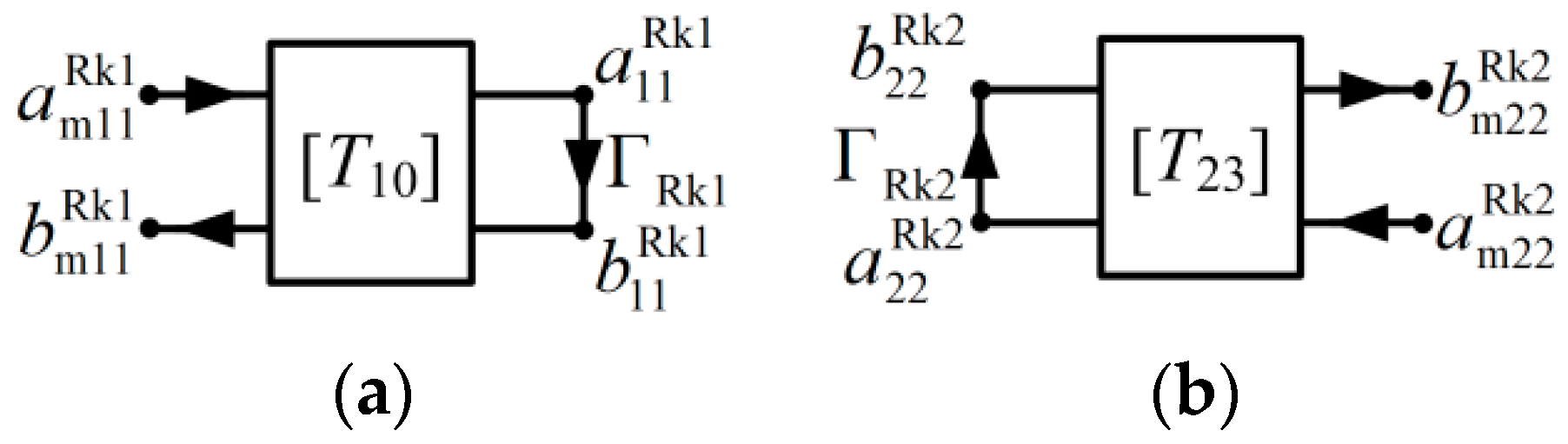
The left and right error boxes are described in the form of T-matrix by (1)–(2), which should be solved during the calibration procedure. Unlike the traditional calibration methods, the proposed algorithm constructs the T-matrix of each error box by measuring two independent single-port standards as shown in Figure 2.

When measuring the single-port standard R_kl (k, l = 1, 2), the error model simplifies to the error box as shown in Figure 2. The subscript of R_kl represents the kth (k = 1, 2…) standard connected to port l (l = 1, 2). The reflection coefficient of R_kl is defined as Γ_Rkl.

By measurements of two single-port standards R₁₁ and R₂₁ at port 1 (Figure 2a), two Equations similar to (1) can be obtained, and after combination the result is shown as follows:

$$\left[\begin{array}{cc}{a}_{11}^{\mathrm{R}11}& a_{11}^{\mathrm{R}21}\\ {\mathrm{\Gamma }}_{\mathrm{R}11}{a}_{11}^{\mathrm{R}11}& {\mathrm{\Gamma }}_{\mathrm{R}21}{a}_{11}^{\mathrm{R}21}\end{array}\right]=[T_{10}]\left[\begin{array}{cc}{a}_{\mathrm{m}11}^{\mathrm{R}11}& a_{\mathrm{m}11}^{\mathrm{R}21}\\ b_{\mathrm{m}11}^{\mathrm{R}11}& b_{\mathrm{m}11}^{\mathrm{R}21}\end{array}\right].$$

(4)

Similarly, measurements of two single-port standards R₁₂ and R₂₂ at port 2 (Figure 2b) generate the following Equation:

$$\left[\begin{array}{cc}{a}_{22}^{\mathrm{R}12}& a_{22}^{\mathrm{R}22}\\ {\mathrm{\Gamma }}_{\mathrm{R}12}{a}_{22}^{R12}& {\mathrm{\Gamma }}_{\mathrm{R}22}{a}_{22}^{\mathrm{R}22}\end{array}\right]=[T_{23}]\left[\begin{array}{cc}{a}_{\mathrm{m}22}^{\mathrm{R}12}& a_{\mathrm{m}22}^{\mathrm{R}22}\\ b_{\mathrm{m}22}^{\mathrm{R}12}& b_{\mathrm{m}22}^{\mathrm{R}22}\end{array}\right].$$

(5)

Based on (4) and (5), the T-matrices of error boxes can be rewritten as follows:

$$[T_{10}]=a_{11}^{\mathrm{R}11}\left[\begin{array}{cc}1& x\\ {\mathrm{\Gamma }}_{\mathrm{R}11}& {\mathrm{\Gamma }}_{\mathrm{R}21}x\end{array}\right]{\left[\begin{array}{cc}{a}_{\mathrm{m}11}^{\mathrm{R}11}& a_{\mathrm{m}11}^{\mathrm{R}21}\\ b_{\mathrm{m}11}^{\mathrm{R}11}& b_{\mathrm{m}11}^{\mathrm{R}21}\end{array}\right]}^{-1}$$

(6)

$$[T_{23}]=\frac{a_{11}^{\mathrm{R}11}}{z}\left[\begin{array}{cc}1& y\\ {\mathrm{\Gamma }}_{\mathrm{R}12}& {\mathrm{\Gamma }}_{\mathrm{R}22}y\end{array}\right]{\left[\begin{array}{cc}{a}_{\mathrm{m}22}^{\mathrm{R}12}& a_{\mathrm{m}22}^{\mathrm{R}22}\\ b_{\mathrm{m}22}^{\mathrm{R}12}& b_{\mathrm{m}22}^{\mathrm{R}22}\end{array}\right]}^{-1}$$

(7)

where x, y, and z are defined as follows:

$$x=\frac{a_{11}^{\mathrm{R}21}}{a_{11}^{\mathrm{R}11}}$$

(8)

$$y=\frac{a_{22}^{\mathrm{R}22}}{a_{22}^{\mathrm{R}12}}$$

(9)

$$z=\frac{a_{11}^{\mathrm{R}11}}{a_{22}^{\mathrm{R}12}}.$$

(10)

As shown in (8)–(10), x, y, and z are the ratios of wave parameters; therefore, we define them as wave ratios in this paper. Meanwhile, because $a_{11}^{\mathrm{R}11}$, $a_{11}^{\mathrm{R}21}$, $a_{22}^{\mathrm{R}12}$, and $a_{22}^{\mathrm{R}22}$ are directly inspired by the stimulated signals, the wave ratios x, y, and z should have nonzero and finite values. Obviously, (6) and (7) contain the information about the standards R_kl (k, l = 1, 2), so no more Equations need to be set up for these standards.

2.2. Establishment of the Calibration Equation

Having obtained the description for [T₁₀], when a single-port standard R_k1 (k >2) is connected to port 1 and is measured by the VNA (Figure 2a), the following Equation is obtained:

$$\left[\begin{array}{c}{a}_{11}^{\mathrm{Rk}1}\\ {\mathrm{\Gamma }}_{\mathrm{Rk}1}{a}_{11}^{\mathrm{Rk}1}\end{array}\right]=[T_{10}]\left[\begin{array}{c}{a}_{\mathrm{m}11}^{\mathrm{Rk}1}\\ b_{\mathrm{m}11}^{\mathrm{Rk}1}\end{array}\right].$$

(11)

Then, substituting (6) into (11) results in the following Equation:

$$\left[\begin{array}{c}{a}_{11}^{\mathrm{Rk}1}\\ {\mathrm{\Gamma }}_{\mathrm{Rk}1}{a}_{11}^{\mathrm{Rk}1}\end{array}\right]=a_{11}^{\mathrm{R}11}\left[\begin{array}{cc}1& x\\ {\mathrm{\Gamma }}_{\mathrm{R}11}& {\mathrm{\Gamma }}_{\mathrm{R}21}x\end{array}\right]{\left[\begin{array}{cc}{a}_{\mathrm{m}11}^{\mathrm{R}11}& a_{\mathrm{m}11}^{\mathrm{R}21}\\ b_{\mathrm{m}11}^{\mathrm{R}11}& b_{\mathrm{m}11}^{\mathrm{R}21}\end{array}\right]}^{-1}\left[\begin{array}{c}{a}_{\mathrm{m}11}^{\mathrm{Rk}1}\\ b_{\mathrm{m}11}^{\mathrm{Rk}1}\end{array}\right].$$

(12)

Based on (12), the calibration Equation for R_k1 (k >2) is given as follows:

$${\mathrm{\Gamma }}_{\mathrm{Rk}1}=\frac{w_1^{\mathrm{Rk}1}{\mathrm{\Gamma }}_{\mathrm{R}11}+w_2^{\mathrm{Rk}1}{\mathrm{\Gamma }}_{\mathrm{R}21}x}{w_1^{\mathrm{Rk}1}+w_2^{\mathrm{Rk}1}x}$$

(13)

where the measurement terms $w_1^{\mathrm{Rk}1}$ and $w_2^{\mathrm{Rk}1}$ are defined as

$$\left[\begin{array}{c}{w}_1^{\mathrm{Rk}1}\\ w_2^{\mathrm{Rk}1}\end{array}\right]={\left[\begin{array}{cc}{a}_{\mathrm{m}11}^{\mathrm{R}11}& a_{\mathrm{m}11}^{\mathrm{R}21}\\ b_{\mathrm{m}11}^{\mathrm{R}11}& b_{\mathrm{m}11}^{\mathrm{R}21}\end{array}\right]}^{-1}\left[\begin{array}{c}{a}_{\mathrm{m}11}^{\mathrm{Rk}1}\\ b_{\mathrm{m}11}^{\mathrm{Rk}1}\end{array}\right].$$

(14)

Similarly, measurement of a single-port standard R_k2 (k >2) (Figure 2b) can generate the following Equation:

$${\mathrm{\Gamma }}_{\mathrm{Rk}2}=\frac{w_1^{\mathrm{Rk}2}{\mathrm{\Gamma }}_{\mathrm{R}12}+w_2^{\mathrm{Rk}2}{\mathrm{\Gamma }}_{\mathrm{R}22}y}{w_1^{\mathrm{Rk}2}+w_2^{\mathrm{Rk}2}y}$$

(15)

where the variables $w_1^{\mathrm{Rk}2}$ and $w_2^{\mathrm{Rk}2}$ are defined by using measurements as shown below.

$$\left[\begin{array}{c}{w}_1^{\mathrm{Rk}2}\\ w_2^{\mathrm{Rk}2}\end{array}\right]={\left[\begin{array}{cc}{a}_{\mathrm{m}22}^{\mathrm{R}12}& a_{\mathrm{m}22}^{\mathrm{R}22}\\ b_{\mathrm{m}22}^{\mathrm{R}12}& b_{\mathrm{m}22}^{\mathrm{R}22}\end{array}\right]}^{-1}\left[\begin{array}{c}{a}_{\mathrm{m}22}^{\mathrm{Rk}2}\\ b_{\mathrm{m}22}^{\mathrm{Rk}2}\end{array}\right]$$

(16)

Besides the calibration Equations (13) and (15) for single-port standards, at least a two-port standard must be introduced in order to complete the two-port VNA calibration. The kth two-port standard L_k (k = 1, 2…) with T-matrix $[T_{12}^{\mathrm{Lk}}]=\left[\begin{array}{cc}{t}_{11}^{\mathrm{Lk}}& t_{12}^{\mathrm{Lk}}\\ t_{21}^{\mathrm{Lk}}& t_{22}^{\mathrm{Lk}}\end{array}\right]$, is measured to continue the calibration as shown in Figure 3.

Figure 3 shows the same model as in Figure 1, but the superscript ‘Lk’ is added to represent the standard L_k. According to (1) and (2), the waves at the ports of L_k in Figure 3 can be combined and expressed by

$$\left[\begin{array}{cc}{a}_{11}^{\mathrm{Lk}}& a_{12}^{\mathrm{Lk}}\\ b_{11}^{\mathrm{Lk}}& b_{12}^{\mathrm{Lk}}\end{array}\right]=[T_{10}]\left[\begin{array}{cc}{a}_{\mathrm{m}11}^{\mathrm{Lk}}& a_{\mathrm{m}12}^{\mathrm{Lk}}\\ b_{\mathrm{m}11}^{\mathrm{Lk}}& b_{\mathrm{m}12}^{\mathrm{Lk}}\end{array}\right]$$

(17)

$$\left[\begin{array}{cc}{a}_{21}^{\mathrm{Lk}}& a_{22}^{\mathrm{Lk}}\\ b_{21}^{\mathrm{Lk}}& b_{22}^{\mathrm{Lk}}\end{array}\right]=[T_{23}]\left[\begin{array}{cc}{a}_{\mathrm{m}21}^{\mathrm{Lk}}& a_{\mathrm{m}22}^{\mathrm{Lk}}\\ b_{\mathrm{m}21}^{\mathrm{Lk}}& b_{\mathrm{m}22}^{\mathrm{Lk}}\end{array}\right].$$

(18)

Based on (3), we can use (17) and (18) to get the following matrix Equation for the two-port standard:

$$[T_{10}]\left[\begin{array}{cc}{a}_{\mathrm{m}11}^{\mathrm{Lk}}& a_{\mathrm{m}12}^{\mathrm{Lk}}\\ b_{\mathrm{m}11}^{\mathrm{Lk}}& b_{\mathrm{m}12}^{\mathrm{Lk}}\end{array}\right]=\left[\begin{array}{cc}0& 1\\ 1& 0\end{array}\right][T_{12}^{\mathrm{Lk}}][T_{23}]\left[\begin{array}{cc}{a}_{\mathrm{m}21}^{\mathrm{Lk}}& a_{\mathrm{m}22}^{\mathrm{Lk}}\\ b_{\mathrm{m}21}^{\mathrm{Lk}}& b_{\mathrm{m}22}^{\mathrm{Lk}}\end{array}\right].$$

(19)

Then, by substituting (6) and (7) into (19), the calibration Equation resulting from L_k is given as follows:

$$\left[\begin{array}{cc}0& 1\\ 1& 0\end{array}\right][T_{12}^{\mathrm{Lk}}]=z\left[\begin{array}{cc}1& 1\\ {\mathrm{\Gamma }}_{\mathrm{R}11}& {\mathrm{\Gamma }}_{\mathrm{R}21}\end{array}\right]\left[\begin{array}{cc}1& 0\\ 0& x\end{array}\right][W_{\mathrm{Lk}}]{\left[\begin{array}{cc}1& 0\\ 0& y\end{array}\right]}^{-1}{\left[\begin{array}{cc}1& 1\\ {\mathrm{\Gamma }}_{\mathrm{R}12}& {\mathrm{\Gamma }}_{\mathrm{R}22}\end{array}\right]}^{-1}$$

(20)

where the matrix [W_Lk] is fully known from measurements as shown below.

$$\begin{array}{ll}[W_{\mathrm{Lk}}]& =\left[\begin{array}{cc}{w}_{11}^{\mathrm{Lk}}& w_{12}^{\mathrm{Lk}}\\ w_{21}^{\mathrm{Lk}}& w_{22}^{\mathrm{Lk}}\end{array}\right]\\ & ={\left[\begin{array}{cc}{a}_{\mathrm{m}11}^{\mathrm{R}11}& a_{\mathrm{m}11}^{\mathrm{R}21}\\ b_{\mathrm{m}11}^{\mathrm{R}11}& b_{\mathrm{m}11}^{\mathrm{R}21}\end{array}\right]}^{-1}\left[\begin{array}{cc}{a}_{\mathrm{m}11}^{\mathrm{Lk}}& a_{\mathrm{m}12}^{\mathrm{Lk}}\\ b_{\mathrm{m}11}^{\mathrm{Lk}}& b_{\mathrm{m}12}^{\mathrm{Lk}}\end{array}\right]{\left[\begin{array}{cc}{a}_{\mathrm{m}21}^{\mathrm{Lk}}& a_{\mathrm{m}22}^{\mathrm{Lk}}\\ b_{\mathrm{m}21}^{\mathrm{Lk}}& b_{\mathrm{m}22}^{\mathrm{Lk}}\end{array}\right]}^{-1}\left[\begin{array}{cc}{a}_{\mathrm{m}22}^{\mathrm{R}12}& a_{\mathrm{m}22}^{\mathrm{R}22}\\ b_{\mathrm{m}22}^{\mathrm{R}12}& b_{\mathrm{m}22}^{\mathrm{R}22}\end{array}\right]\end{array}$$

(21)

The calibration Equation (20) from the two-port standard L_k can also be expanded, and the results are given as follows:

$$\{\begin{array}{l}{t}_{21}^{\mathrm{Lk}}+t_{22}^{\mathrm{Lk}}{\mathrm{\Gamma }}_{\mathrm{R}12}=w_{11}^{\mathrm{Lk}}z+w_{21}^{\mathrm{Lk}}xz\hfill \\ t_{21}^{\mathrm{Lk}}y+t_{22}^{\mathrm{Lk}}{\mathrm{\Gamma }}_{\mathrm{R}22}y=w_{12}^{\mathrm{Lk}}z+w_{22}^{\mathrm{Lk}}xz\hfill \\ t_{11}^{\mathrm{Lk}}+t_{12}^{\mathrm{Lk}}{\mathrm{\Gamma }}_{\mathrm{R}12}=w_{11}^{\mathrm{Lk}}{\mathrm{\Gamma }}_{\mathrm{R}11}z+w_{21}^{\mathrm{Lk}}{\mathrm{\Gamma }}_{\mathrm{R}21}xz\hfill \\ t_{11}^{\mathrm{Lk}}y+t_{12}^{\mathrm{Lk}}{\mathrm{\Gamma }}_{\mathrm{R}22}y=w_{12}^{\mathrm{Lk}}{\mathrm{\Gamma }}_{\mathrm{R}11}z+w_{22}^{\mathrm{Lk}}{\mathrm{\Gamma }}_{\mathrm{R}21}xz\hfill \end{array}.$$

(22)

Equations (13), (15), (20), and (22) are established to solve the unknowns in the calibration algorithm.

2.3. Error Correction for DUT Measurement

According to the above analysis, a two-port DUT measurement will result in a matrix Equation similar to (19). Therefore, the T-matrix of the DUT can be expressed as follows:

$$[T_{12}^{\mathrm{D}}]=\left[\begin{array}{cc}0& 1\\ 1& 0\end{array}\right]\left[T_{10}\right]\left[\begin{array}{cc}{a}_{\mathrm{m}11}^{\mathrm{D}}& a_{\mathrm{m}12}^{\mathrm{D}}\\ b_{\mathrm{m}11}^{\mathrm{D}}& b_{\mathrm{m}12}^{\mathrm{D}}\end{array}\right]{\left[\begin{array}{cc}{a}_{\mathrm{m}21}^{\mathrm{D}}& a_{\mathrm{m}22}^{\mathrm{D}}\\ b_{\mathrm{m}21}^{\mathrm{D}}& b_{\mathrm{m}22}^{\mathrm{D}}\end{array}\right]}^{-1}{[T_{23}]}^{-1}$$

(23)

where $a_{\mathrm{mij}}^{\mathrm{D}}$ and $b_{\mathrm{mij}}^{\mathrm{D}}$ (i, j = 1, 2) are the measured wave parameters of the DUT. After substitution of (6) and (7) in (23), an Equation similar to (20) can be obtained for the corrected $[T_{12}^{\mathrm{D}}]$ as shown below.

$$[T_{12}^{\mathrm{D}}]=z\left[\begin{array}{cc}{\mathrm{\Gamma }}_{\mathrm{R}11}& {\mathrm{\Gamma }}_{\mathrm{R}21}x\\ 1& x\end{array}\right][W_{\mathrm{D}}]{\left[\begin{array}{cc}1& y\\ {\mathrm{\Gamma }}_{\mathrm{R}12}& {\mathrm{\Gamma }}_{\mathrm{R}22}y\end{array}\right]}^{-1}$$

(24)

The matrix [W_D] with the same form of (21) is obtained from measurement. From the above results, it is easy to find out that the elements of [T₁₀] and [T₂₃] must be known except a common factor $a_{11}^{\mathrm{R}11}$. A knowledge of $a_{11}^{\mathrm{R}11}$ is not required for the de-embedding or calibration task, therefore one may arbitrarily set it to any nonzero value. In this work, we set

$$a_{11}^{\mathrm{R}11}=\sqrt{\frac{a_{\mathrm{m}11}^{\mathrm{R}11}{b}_{\mathrm{m}11}^{\mathrm{R}21}-a_{\mathrm{m}11}^{\mathrm{R}21}{b}_{\mathrm{m}11}^{\mathrm{R}11}}{{(\mathrm{\Gamma }}_{\mathrm{R}21}-{\mathrm{\Gamma }}_{\mathrm{R}11})x}}.$$

(25)

Equation (25) can make the determinant of [T₁₀] equal to 1, which does not mean that the real error box is reciprocal. Substituting (25) into (6) and (7) can conclude

$$[T_{10}]=\sqrt{\frac{a_{\mathrm{m}11}^{\mathrm{R}11}{b}_{\mathrm{m}11}^{\mathrm{R}21}-a_{\mathrm{m}11}^{\mathrm{R}21}{b}_{\mathrm{m}11}^{\mathrm{R}11}}{{(\mathrm{\Gamma }}_{\mathrm{R}21}-{\mathrm{\Gamma }}_{\mathrm{R}11})x}}\left[\begin{array}{cc}1& x\\ {\mathrm{\Gamma }}_{\mathrm{R}11}& {\mathrm{\Gamma }}_{\mathrm{R}21}x\end{array}\right]{\left[\begin{array}{cc}{a}_{\mathrm{m}11}^{\mathrm{R}11}& a_{\mathrm{m}11}^{\mathrm{R}21}\\ b_{\mathrm{m}11}^{\mathrm{R}11}& b_{\mathrm{m}11}^{\mathrm{R}21}\end{array}\right]}^{-1}$$

(26)

$$[T_{23}]=\frac{1}{z}\sqrt{\frac{a_{\mathrm{m}11}^{\mathrm{R}11}{b}_{\mathrm{m}11}^{\mathrm{R}21}-a_{\mathrm{m}11}^{\mathrm{R}21}{b}_{\mathrm{m}11}^{\mathrm{R}11}}{{(\mathrm{\Gamma }}_{\mathrm{R}21}-{\mathrm{\Gamma }}_{\mathrm{R}11})x}}\left[\begin{array}{cc}1& y\\ {\mathrm{\Gamma }}_{\mathrm{R}12}& {\mathrm{\Gamma }}_{\mathrm{R}22}y\end{array}\right]{\left[\begin{array}{cc}{a}_{\mathrm{m}22}^{\mathrm{R}12}& a_{\mathrm{m}22}^{\mathrm{R}22}\\ b_{\mathrm{m}22}^{\mathrm{R}12}& b_{\mathrm{m}22}^{\mathrm{R}22}\end{array}\right]}^{-1}.$$

(27)

To determine [T₁₀] and [T₂₃], besides the definition and measurement of standards R_kl (k, l = 1, 2), only the newly introduced x, y, and z are required to be solved. Once the unknowns in (26) and (27) are all determined, the T-matrix of the DUT can be corrected by (23), and then the following Equation can be used for the S-matrix transformation:

$$[S]={\left(\left[\begin{array}{cc}1& 0\\ 0& 0\end{array}\right]-[T_{12}^{\mathrm{D}}]\left[\begin{array}{cc}0& 0\\ 0& 1\end{array}\right]\right)}^{-1}\left([T_{12}^{\mathrm{D}}]\left[\begin{array}{cc}0& 1\\ 0& 0\end{array}\right]-\left[\begin{array}{cc}0& 0\\ 1& 0\end{array}\right]\right)$$

(28)

where [S] is defined as the S-matrix of the DUT.

The T-matrix representation of error boxes can be also converted into the cascade matrix form defined in [6] by using the following Equations:

$$[R_{\mathrm{left}}]=\left[\begin{array}{cc}0& 1\\ 1& 0\end{array}\right]{[T_{10}]}^{-1}\left[\begin{array}{cc}0& 1\\ 1& 0\end{array}\right]$$

(29)

$$[R_{\mathrm{right}}]=[T_{23}]$$

(30)

where [R_left] and [R_right] are the cascade matrix of the left error box and the reverse cascade matrix of the right error box, respectively.

3. LRM/LRMM/LRRM Deviation

This section determines the elements of [T₁₀] and [T₂₃] in (26) and (27) by means of LRM, LRMM, and LRRM calibrations. For the self-calibration methods LRM/LRMM/LRRM, not only the wave ratios but also the unknown reflection coefficients of the single-port standards need to be determined. To make a clear distinction among LRM/LRMM/LRRM, the used standards are shown in

Table 1. Standards used for LRM/LRMM/LRRM.

	Standard	Single-Port Standard		Two-Port Standard Lk
Algorithm		Rk1 at Port 1	Rk2 at Port 2
LRM		R (×), M (√)	R (×), M (√)	L (√)
LRMM		R (×), M1 (√)	R (×), M2 (√)	L (√)
LRRM		R1 (×), R2 (×), M (?)	R1 (×), R2 (×)	L (√)

LRM: line-reflect-match; LRMM: line-reflect-match-match; LRRM: line-reflect-reflect-match; √: known; ×: unknown; ?: partially known.

. For a certain calibration method, the independent standards at each port are distinguished by using different characters or numbers. The symmetrical standards with identical reflection coefficient are represented by identical characters and numbers. The detailed summary of LRM/LRMM/LRRM calibrations can be found in Table 2 of Ref. [1].

The symbol ‘√’ means that the network parameters of a standard are completely known, whereas the symbol ‘×’ means that the network parameters are unknown but the sign can be identified by using the inductive or capacitive property. The symbol ‘?’ means that the standard is partially known. For the match standard (M) used in LRRM, only its direct current (DC) resistance is known and its parasitic inductance and capacitance are to be determined [26], as a result, this standard is denoted by the ‘?’ symbol. In this work, the standard L represents an arbitrary two-port device with completely-known property rather than a perfect thru or a line.

Based on the theory given in section II, the formulation of LRM/LRMM/LRRM calibration algorithms is described in detail below.

3.1. LRM Derivation

As shown in Table 1, the LRM calibration uses a known two-port standard L (L₁), unknown symmetrical reflection standards R (R₁₁/R₁₂), and known symmetrical match standards M (R₂₁/R₂₂). The reflection coefficients of R and M are defined as Γ_R and Γ_M, respectively. With Γ_R11 = Γ_R12 = Γ_R and Γ_R21 = Γ_R22 = Γ_M, the T-matrices [T₁₀] and [T₂₃] can be constructed by using (6) and (7) through the measurements of R and M. After that, only the following Equation needs to be built by using (20) to implement the LRM algorithm.

$$\left[\begin{array}{cc}0& 1\\ 1& 0\end{array}\right][T_{12}^{\mathrm{L}}]=z\left[\begin{array}{cc}1& 1\\ {\mathrm{\Gamma }}_{\mathrm{R}}& {\mathrm{\Gamma }}_{\mathrm{M}}\end{array}\right]\left[\begin{array}{cc}1& 0\\ 0& x\end{array}\right][W_{\mathrm{L}}]{\left[\begin{array}{cc}1& 0\\ 0& y\end{array}\right]}^{-1}{\left[\begin{array}{cc}1& 1\\ {\mathrm{\Gamma }}_{\mathrm{R}}& {\mathrm{\Gamma }}_{\mathrm{M}}\end{array}\right]}^{-1}$$

(31)

The T-matrix $[T_{12}^{\mathrm{L}}]$ of standard L and the reflection coefficient Γ_M are known from their definition, meanwhile, the matrix [W_L] with the same form of (21) can be obtained by measurement. The unknown reflection coefficient Γ_R and the wave ratios x, y, and z need to be solved by (31) before the error correction. To simplify the calculation, the determinant and trace conservation of (31) result in the following Equations:

$$\frac{x}{y}{z}^2=-\frac{\left|[T_{12}^{\mathrm{L}}]\right|}{\left|[W_{\mathrm{L}}]\right|}$$

(32)

$$w_{11}^{\mathrm{L}}z+w_{22}^{\mathrm{L}}\frac{x}{y}z=t_{21}^{\mathrm{L}}+t_{12}^{\mathrm{L}}$$

(33)

where $w_{\mathrm{ij}}^{\mathrm{L}}$ and $t_{\mathrm{ij}}^{\mathrm{L}}$ are defined as the (i, j)th element of [W_L] and $[T_{12}^{\mathrm{L}}]$, respectively. If any reciprocal device is used as the standard L, the determinant $\left|[T_{12}^{\mathrm{L}}]\right|$ equals one and (32) could be further simplified. Multiplying both sides of (33) by z and substituting (32) into the result leads to the following quadratic Equation about z:

$$c_2{z}^2+c_{1}z+c_0=0.$$

(34)

The coefficients are known and expressed by

$$\{\begin{array}{l}{c}_2=w_{11}^{\mathrm{L}}\hfill \\ c_1=-t_{21}^{\mathrm{L}}-t_{12}^{\mathrm{L}}\hfill \\ c_0=-\frac{w_{22}^{\mathrm{L}}\left|[T_{12}^{\mathrm{L}}]\right|}{\left|[W_{\mathrm{L}}]\right|}\hfill \end{array}.$$

(35)

As a result, the wave ratio z can be solved directly from (34) as follows:

$$z=\frac{-c_1\pm \sqrt{c_1^2-4c_2{c}_0}}{2c_2}.$$

(36)

The root of z is selected later by the corrected Γ_R. Besides, if any uniform line is selected as the standard L, the right term in (33) equals zero and (34) could be reduced. However, in this work, the algorithm can use an arbitrary known two-port device as the line standard L, rather than the perfect thru or line, which adds to the versatility of the proposed theory. Substituting (36) into (32) can calculate

$$\frac{x}{y}z=-\frac{\left|[T_{12}^{\mathrm{L}}]\right|}{\left|[W_{\mathrm{L}}]\right|z}.$$

(37)

Based on (36) and (37), and similar to (22), (31) is expanded and the following Equations are obtained:

$$\left[\begin{array}{cc}{t}_{22}^{\mathrm{L}}& -w_{21}^{{}^{\prime }\mathrm{L}}\\ 0& t_{21}^{\mathrm{L}}+t_{22}^{\mathrm{L}}{\mathrm{\Gamma }}_{\mathrm{M}}-w_{22}^{{}^{\prime }\mathrm{L}}\\ w_{11}^{{}^{\prime }\mathrm{L}}-t_{12}^{\mathrm{L}}& w_{21}^{{}^{\prime }\mathrm{L}}{\mathrm{\Gamma }}_{\mathrm{M}}\\ w_{12}^{{}^{\prime }\mathrm{L}}& w_{22}^{{}^{\prime }\mathrm{L}}{\mathrm{\Gamma }}_{\mathrm{M}}-t_{11}^{\mathrm{L}}-t_{12}^{\mathrm{L}}{\mathrm{\Gamma }}_{\mathrm{M}}\end{array}\right]\left[\begin{array}{c}{\mathrm{\Gamma }}_{\mathrm{R}}\\ x\end{array}\right]=\left[\begin{array}{c}{w}_{11}^{{}^{\prime }\mathrm{L}}-t_{21}^{\mathrm{L}}\\ w_{12}^{{}^{\prime }\mathrm{L}}\\ t_{11}^{\mathrm{L}}\\ 0\end{array}\right]$$

(38)

where the known variables are defined as

$$\{\begin{array}{l}{w}_{11}^{{}^{\prime }\mathrm{L}}=w_{11}^{\mathrm{L}}z\\ w_{21}^{{}^{\prime }\mathrm{L}}=w_{21}^{\mathrm{L}}z\\ w_{12}^{{}^{\prime }\mathrm{L}}=w_{12}^{\mathrm{L}}\frac{x}{y}z\\ w_{22}^{{}^{\prime }\mathrm{L}}=w_{22}^{\mathrm{L}}\frac{x}{y}z\end{array}.$$

(39)

Based on the first two Equations of (38), x and Γ_R can be determined by

$$x=\frac{w_{12}^{{}^{\prime }\mathrm{L}}}{t_{21}^{\mathrm{L}}+t_{22}^{\mathrm{L}}{\mathrm{\Gamma }}_{\mathrm{M}}-w_{22}^{{}^{\prime }\mathrm{L}}}$$

(40)

$${\mathrm{\Gamma }}_{\mathrm{R}}=\frac{w_{11}^{{}^{\prime }\mathrm{L}}-t_{21}^{\mathrm{L}}+w_{21}^{{}^{\prime }\mathrm{L}}x}{t_{22}^{\mathrm{L}}}.$$

(41)

Substituting (36) and (40) into (37) results in the solution for wave ratio y:

$$y=-\frac{\left|[W_{\mathrm{L}}]\right|}{\left|[T_{12}^{\mathrm{L}}]\right|}x{z}^2.$$

(42)

At this stage, all the unknown variables Γ_R, x, y, and z have been calculated, so the LRM calibration is done.

3.2. LRMM Derivation

Different from the LRM calibration shown in Table 1, in LRMM calibration, the asymmetrical match standards M₁ (R₂₁) and M₂ (R₂₂), with known reflection coefficients Γ_M1 and Γ_M2, are used to construct the T-matrices of error boxes. Similar to (31), the calibration Equation resulting from measurement of the two-port standard L is easily given as below:

$$\left[\begin{array}{cc}0& 1\\ 1& 0\end{array}\right][T_{12}^{\mathrm{L}}]=z\left[\begin{array}{cc}1& 1\\ {\mathrm{\Gamma }}_{\mathrm{R}}& {\mathrm{\Gamma }}_{\mathrm{M}1}\end{array}\right]\left[\begin{array}{cc}1& 0\\ 0& x\end{array}\right][W_{\mathrm{L}}]{\left[\begin{array}{cc}1& 0\\ 0& y\end{array}\right]}^{-1}{\left[\begin{array}{cc}1& 1\\ {\mathrm{\Gamma }}_{\mathrm{R}}& {\mathrm{\Gamma }}_{\mathrm{M}2}\end{array}\right]}^{-1}.$$

(43)

The trace conservation cannot be used anymore, so similar to (22), (43) is expanded and the result is shown as follows:

$$\left[\begin{array}{ccc}{w}_{21}^{\mathrm{L}}& 0& w_{11}^{\mathrm{L}}\\ w_{22}^{\mathrm{L}}& -t_{21}^{\mathrm{L}}-t_{22}^{\mathrm{L}}{\mathrm{\Gamma }}_{\mathrm{M}2}& w_{12}^{\mathrm{L}}\\ w_{21}^{\mathrm{L}}{\mathrm{\Gamma }}_{\mathrm{M}1}& 0& w_{11}^{\mathrm{L}}{\mathrm{\Gamma }}_{\mathrm{R}}\\ w_{22}^{\mathrm{L}}{\mathrm{\Gamma }}_{\mathrm{M}1}& -t_{11}^{\mathrm{L}}-t_{12}^{\mathrm{L}}{\mathrm{\Gamma }}_{\mathrm{M}2}& w_{12}^{\mathrm{L}}{\mathrm{\Gamma }}_{\mathrm{R}}\end{array}\right]\left[\begin{array}{c}xz\\ y\\ z\end{array}\right]=\left[\begin{array}{c}{t}_{21}^{\mathrm{L}}+t_{22}^{\mathrm{L}}{\mathrm{\Gamma }}_{\mathrm{R}}\\ 0\\ t_{11}^{\mathrm{L}}+t_{12}^{\mathrm{L}}{\mathrm{\Gamma }}_{\mathrm{R}}\\ 0\end{array}\right].$$

(44)

By solving the first three equations of (44), expressions for xz, y, and z in function of Γ_R are obtained. These expressions are plugged into the last equation of (44) to obtain a quadratic equation about Γ_R as shown below:

$$d_2{\mathrm{\Gamma }}_{\mathrm{R}}^2+d_1{\mathrm{\Gamma }}_{\mathrm{R}}+d_0=0$$

(45)

where the coefficients are known and given by

$$\{\begin{array}{ll}{d}_2=& w_{11}^{\mathrm{L}}{w}_{22}^{\mathrm{L}}{t}_{22}^{\mathrm{L}}(t_{11}^{\mathrm{L}}-t_{21}^{\mathrm{L}}{\mathrm{\Gamma }}_{\mathrm{M}1}+t_{12}^{\mathrm{L}}{\mathrm{\Gamma }}_{\mathrm{M}2}-t_{22}^{\mathrm{L}}{\mathrm{\Gamma }}_{\mathrm{M}1}{\mathrm{\Gamma }}_{\mathrm{M}2})\\ & -w_{21}^{\mathrm{L}}{w}_{12}^{\mathrm{L}}(t_{21}^{\mathrm{L}}+t_{22}^{\mathrm{L}}{\mathrm{\Gamma }}_{\mathrm{M}2})(t_{12}^{\mathrm{L}}-t_{22}^{\mathrm{L}}{\mathrm{\Gamma }}_{\mathrm{M}1})\\ d_1=& w_{11}^{\mathrm{L}}{w}_{22}^{\mathrm{L}}(t_{21}^{\mathrm{L}}-t_{12}^{\mathrm{L}})(t_{11}^{\mathrm{L}}-t_{21}^{\mathrm{L}}{\mathrm{\Gamma }}_{\mathrm{M}1}+t_{12}^{\mathrm{L}}{\mathrm{\Gamma }}_{\mathrm{M}2}-t_{22}^{\mathrm{L}}{\mathrm{\Gamma }}_{\mathrm{M}1}{\mathrm{\Gamma }}_{\mathrm{M}2})\\ & -w_{21}^{\mathrm{L}}{w}_{12}^{\mathrm{L}}[(t_{11}^{\mathrm{L}}-t_{21}^{\mathrm{L}}{\mathrm{\Gamma }}_{\mathrm{M}1})(t_{21}^{\mathrm{L}}+t_{22}^{\mathrm{L}}{\mathrm{\Gamma }}_{\mathrm{M}2})\\ & -(t_{11}^{\mathrm{L}}+t_{12}^{\mathrm{L}}{\mathrm{\Gamma }}_{\mathrm{M}2})(t_{12}^{\mathrm{L}}-t_{22}^{\mathrm{L}}{\mathrm{\Gamma }}_{\mathrm{M}1})]\\ d_0=& -w_{11}^{\mathrm{L}}{w}_{22}^{\mathrm{L}}{t}_{11}^{\mathrm{L}}(t_{11}^{\mathrm{L}}-t_{21}^{\mathrm{L}}{\mathrm{\Gamma }}_{\mathrm{M}1}+t_{12}^{\mathrm{L}}{\mathrm{\Gamma }}_{\mathrm{M}2}-t_{22}^{\mathrm{L}}{\mathrm{\Gamma }}_{\mathrm{M}1}{\mathrm{\Gamma }}_{\mathrm{M}2})\\ & +w_{21}^{\mathrm{L}}{w}_{12}^{\mathrm{L}}(t_{11}^{\mathrm{L}}-t_{21}^{\mathrm{L}}{\mathrm{\Gamma }}_{\mathrm{M}1})(t_{11}^{\mathrm{L}}+t_{12}^{\mathrm{L}}{\mathrm{\Gamma }}_{\mathrm{M}2})\end{array}.$$

(46)

Once Γ_R is solved after a root choice, the wave ratios x, y, and z can be calculated by (44) and the LRMM calibration is completed.

3.3. LRRM Derivation

Based on the above LRM and LRMM calibration algorithms, a similar algorithm is developed for LRRM calibration. As shown in Table 1, a two-port standard L (L₁) and single-port standards R₁ (R₁₁/R₁₂), R₂ (R₂₁/R₂₂), and M (R₃₁) are used. Here, R₁ and R₂ are assumed to be the short with the unknown reflection coefficient Γ_R1 and the open standard with Γ_R2, respectively. With Γ_R11 = Γ_R12 = Γ_R1 and Γ_R21 = Γ_R22= Γ_R2, R₁ and R₂ are used to construct the T-matrices of error boxes by (6) and (7). Different from LRM, the reflection coefficient Γ_M of the match standard M is not fully known. With Γ_Rk1 = Γ_M (k = 3), applying (13) results in the following Equation:

$${\mathrm{\Gamma }}_{\mathrm{M}}=\frac{w_1^{\mathrm{M}}{\mathrm{\Gamma }}_{\mathrm{R}1}+w_2^{\mathrm{M}}{\mathrm{\Gamma }}_{\mathrm{R}2}x}{w_1^{\mathrm{M}}+w_2^{\mathrm{M}}x}$$

(47)

where the measurement terms $w_1^{\mathrm{M}}$ and $w_2^{\mathrm{M}}$ are defined similar to (14). Meanwhile, based on (20), the measurement of the two-port standard L can generate the following Equation:

$$\left[\begin{array}{cc}0& 1\\ 1& 0\end{array}\right][T_{12}^{\mathrm{L}}]=z\left[\begin{array}{cc}1& 1\\ {\mathrm{\Gamma }}_{\mathrm{R}1}& {\mathrm{\Gamma }}_{\mathrm{R}2}\end{array}\right]\left[\begin{array}{cc}1& 0\\ 0& x\end{array}\right][W_{\mathrm{L}}]{\left[\begin{array}{cc}1& 0\\ 0& y\end{array}\right]}^{-1}{\left[\begin{array}{cc}1& 1\\ {\mathrm{\Gamma }}_{\mathrm{R}1}& {\mathrm{\Gamma }}_{\mathrm{R}2}\end{array}\right]}^{-1}.$$

(48)

From (21), we know that the matrix [W_L] can be gained by measurement. Also, the T-matrix $[T_{12}^{\mathrm{L}}]$ is known from the definition of the standard L. However, for the unknowns, not only the wave ratios x, y, and z, but also the reflection coefficients Γ_R1, Γ_R2, and Γ_M need to be solved before the error correction. Similar to the analysis in LRM calibration, we can obtain the same results as shown in (32)–(37) by using the determinant and trace conservation for (48). To ensure that the analysis is complete and concise, only two formulas are repeated and given below:

$$z=\frac{-c_1\pm \sqrt{c_1^2-4c_2{c}_0}}{2c_2}$$

(49)

$$\frac{x}{y}z=-\frac{\left|[T_{12}^{\mathrm{L}}]\right|}{\left|[W_{\mathrm{L}}]\right|z}.$$

(50)

The variables on the right side of (49) have been defined in (35). Equations (49) and (50) are plugged into (48), and after a similar expansion as in (22), the resulting matrix Equation is shown as follows:

$$\left[\begin{array}{cc}{t}_{22}^{\mathrm{L}}& -w_{21}^{{}^{\prime }\mathrm{L}}\\ 0& t_{21}^{\mathrm{L}}+t_{22}^{\mathrm{L}}{\mathrm{\Gamma }}_{\mathrm{R}2}-w_{22}^{{}^{\prime }\mathrm{L}}\\ w_{11}^{{}^{\prime }\mathrm{L}}-t_{12}^{\mathrm{L}}& w_{21}^{{}^{\prime }\mathrm{L}}{\mathrm{\Gamma }}_{\mathrm{R}2}\\ w_{12}^{{}^{\prime }\mathrm{L}}& w_{22}^{{}^{\prime }\mathrm{L}}{\mathrm{\Gamma }}_{\mathrm{R}2}-t_{11}^{\mathrm{L}}-t_{12}^{\mathrm{L}}{\mathrm{\Gamma }}_{\mathrm{R}2}\end{array}\right]\left[\begin{array}{c}{\mathrm{\Gamma }}_{\mathrm{R}1}\\ x\end{array}\right]=\left[\begin{array}{c}{w}_{11}^{{}^{\prime }\mathrm{L}}-t_{21}^{\mathrm{L}}\\ w_{12}^{{}^{\prime }\mathrm{L}}\\ t_{11}^{\mathrm{L}}\\ 0\end{array}\right]$$

(51)

where the known variables $w_{\mathrm{ij}}^{{}^{\prime }\mathrm{L}}$ (i, j = 1, 2) are defined in (39). From the first two equations of (51), Γ_R1 and x are solved as function of Γ_R2, and the results are as follows:

$$x=\frac{w_{12}^{{}^{\prime }\mathrm{L}}}{t_{21}^{\mathrm{L}}+t_{22}^{\mathrm{L}}{\mathrm{\Gamma }}_{\mathrm{R}2}-w_{22}^{{}^{\prime }\mathrm{L}}}$$

(52)

$${\mathrm{\Gamma }}_{\mathrm{R}1}=\frac{(w_{11}^{{}^{\prime }\mathrm{L}}-t_{21}^{\mathrm{L}})(t_{21}^{\mathrm{L}}+t_{22}^{\mathrm{L}}{\mathrm{\Gamma }}_{\mathrm{R}2}-w_{22}^{{}^{\prime }\mathrm{L}})+w_{21}^{{}^{\prime }\mathrm{L}}{w}_{12}^{{}^{\prime }\mathrm{L}}}{t_{22}^{\mathrm{L}}(t_{21}^{\mathrm{L}}+t_{22}^{\mathrm{L}}{\mathrm{\Gamma }}_{\mathrm{R}2}-w_{22}^{{}^{{}^{\prime }}\mathrm{L}})}.$$

(53)

Then, by substituting (52) and (53) into (47), the following first-order rational expression about Γ_R2 is obtained:

$${\mathrm{\Gamma }}_{\mathrm{M}}=\frac{f_1{\mathrm{\Gamma }}_{\mathrm{R}2}+f_0}{e_1{\mathrm{\Gamma }}_{\mathrm{R}2}+e_0}.$$

(54)

The coefficients in (54) are all known by calibration standard definitions and the measurement quantities as shown below.

$$\{\begin{array}{l}{e}_1={(t_{22}^{\mathrm{L}})}^2{w}_1^{\mathrm{M}}\\ e_0=t_{22}^{\mathrm{L}}(t_{21}^{\mathrm{L}}-w_{22}^{{}^{\prime }\mathrm{L}})w_1^{\mathrm{M}}+t_{22}^{\mathrm{L}}{w}_2^{\mathrm{M}}{w}_{12}^{{}^{\prime }\mathrm{L}}\\ f_1=t_{22}^{\mathrm{L}}(w_{11}^{{}^{\prime }\mathrm{L}}-t_{21}^{\mathrm{L}})w_1^{\mathrm{M}}+t_{22}^{\mathrm{L}}{w}_2^{\mathrm{M}}{w}_{12}^{{}^{\prime }\mathrm{L}}\\ f_0=(w_{11}^{{}^{\prime }\mathrm{L}}-t_{21}^{\mathrm{L}})(t_{21}^{\mathrm{L}}-w_{22}^{{}^{\prime }\mathrm{L}})w_1^{\mathrm{M}}+w_1^{\mathrm{M}}{w}_{21}^{{}^{\prime }\mathrm{L}}{w}_{12}^{{}^{\prime }\mathrm{L}}\end{array}$$

(55)

The broadband reflection coefficient of the match standard, Γ_M is determined from the relationship between Γ_R2 and Γ_M by (54). Similar to the previous work [26], the impedance of the match standard at low frequencies is approximated by its DC resistance, which then allows the open capacitance to be determined at low frequencies. Once the open capacitance is known, the broadband reflection coefficient of the match standard Γ_M can be calculated. A nonlinear fitting is performed for fitting Γ_M with a physical load model [26]. The fitting returns the parasitic load inductance and capacitance, which then allows the fitted Γ_M.fit to be calculated. Γ_M.fit is used as the load definition. The rest of the unknown variables Γ_R2, Γ_R1, x, y, and z can be subsequently calculated. At this point, the LRRM calibration is done.

4. Measurements

On-wafer measurements were performed with a broadband VNA from 0.5 GHz to 110 GHz. One hundred micrometer (100 μm) pitch wafer probes and a commercial impedance standard substrate (ISS) CS-5 (GGB industries, Inc.) were used. On CS-5, there are short, open match standards, and 50 Ω lines of multiple lengths, required by multiline thru-reflect-line (MTRL) calibration [27]. The calibrations proposed in this work are compared with MTRL calibration in order to assess their accuracy. The line lengths are 200 μm, 500 μm, 550 μm, 1000 μm, 1500 μm, and 6000 μm. The on-wafer short standards are used as the short for the calibrations, but open is realized by lifting the wafer probes in air. The different match standards have DC resistances ranging from 12.5 Ω to 100 Ω. An LRM calibration was performed with the 200 μm line, open, and a pair of 50 Ω loads. An LRMM calibration was performed with the 200 μm line, open, and a 50 Ω load at port 1 and a 100 Ω load at port 2. An LRRM calibration was performed with the 200 μm line, on-wafer short, open, and a 50 Ω load at port 1. The reference plane for these calibrations is at the probe-tip.

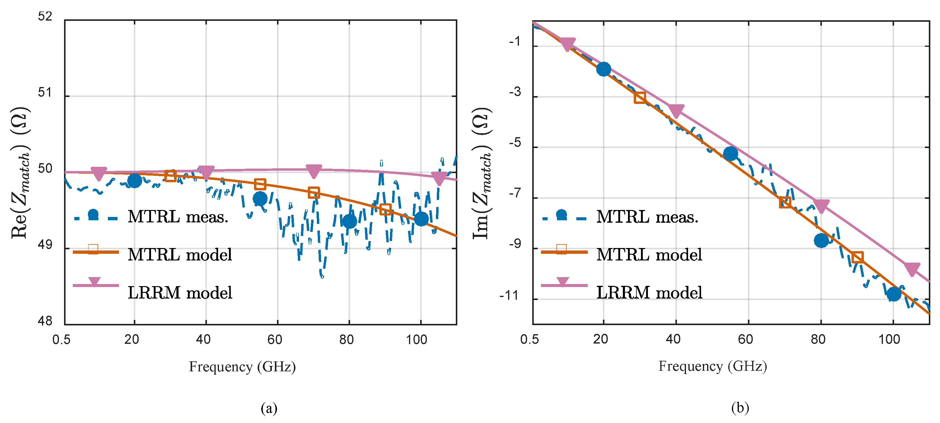
Since LRM and LRMM calibrations require known match standards, the match standards are first characterized using on-wafer MTRL. Figure 4 and Figure 5 show the measured match impedances of the 50 Ω and 100 Ω loads, respectively.

In Figure 4 and Figure 5, the measured load impedances are fitted to a physical load model which takes into account the parasitic inductance and capacitance of shunt loads [26]. The close agreement between the measured (circles) and fitted (squares) values shows that the physical model is sufficient in describing the dispersion in the match impedances up to 110 GHz. The fitted match impedances are used as match definitions for LRM and LRMM calibrations. The triangles in Figure 4 indicate the extracted load impedances from LRRM calibrations. They also show a close match with the impedances from MTRL calibrations, which proves the validity of the proposed LRRM in terms of shunt load characterization.

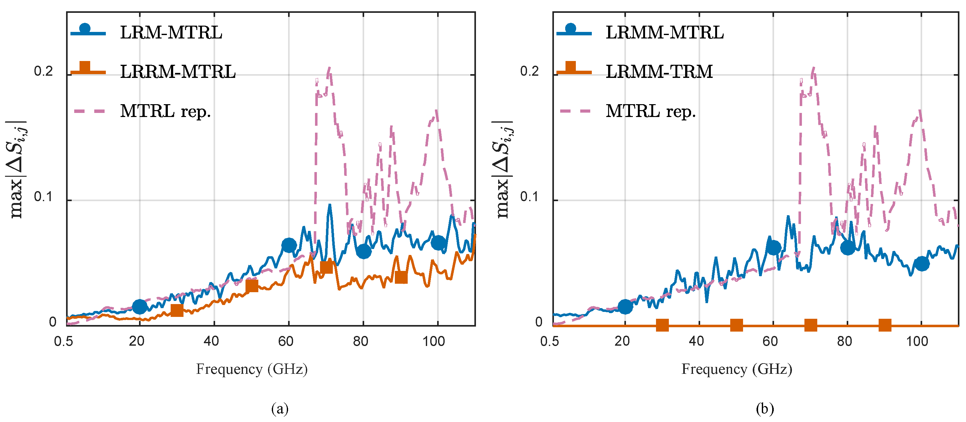
The LRM, LRMM, and LRRM calibrations are compared with on-wafer MTRL calibrations using the calibration comparison technique [28]. Calibration comparison is a known method for comparing two calibrations. The method calculates the maximum deviation in calibrated S-parameters (max|ΔS_{i, j}|_{i, j=1 or 2}) of an arbitrary passive DUT. The error boxes [T₁₀] and [T₂₃] are transformed into the cascade matrices defined in [6] and then compared with the error boxes from MTRL calibrations. The calibration comparison results of LRM and LRRM are shown in Figure 6a. The proposed LRM and LRRM calibrations show relatively low deviations from MTRL calibration, compared to the repeatability of MTRL calibration. Figure 6b shows the comparison between the LRMM, TRM, and MTRL calibrations. The proposed LRMM gives exactly the same calibration coefficients as the state-of-the-art TRM method [14], and shows small deviation from the reference MTRL. As a conclusion, LRM, LRMM, and LRRM all show good accuracies up to 110 GHz.

5. Conclusions

This paper develops a theory for reformulations of LRM/LRMM/LRRM calibrations. By using single-port measurements to construct the T-matrices of error boxes, only three wave ratios need to be defined, and the number of Equations involved in the calculation process is largely reduced. In addition, the two-port standard L is not limited to the perfect thru or line. Instead, an arbitrary two-port device with known properties can be used. Based on this new theory, the analytical formulas for LRM, LRMM, and LRRM calibrations are derived and successfully verified by experiments.