Effect of Ultrafast Imaging on Shear Wave Visualization and Characterization: An Experimental and Computational Study in a Pediatric Ventricular Model

Featured Application

Clinical application of Shear Wave Elastography for cardiac stiffness assessment in children.

Abstract

Plane wave imaging in Shear Wave Elastography (SWE) captures shear wave propagation in real-time at ultrafast frame rates. To assess the capability of this technique in accurately visualizing the underlying shear wave mechanics, this work presents a multiphysics modeling approach providing access to the true biomechanical wave propagation behind the virtual image. This methodology was applied to a pediatric ventricular model, a setting shown to induce complex shear wave propagation due to geometry. Phantom experiments are conducted in support of the simulations. The model revealed that plane wave imaging altered the visualization of the shear wave pattern in the time (broadened front and negatively biased velocity estimates) and frequency domain (shifted and/or decreased signal frequency content). Furthermore, coherent plane wave compounding (effective frame rate of 2.3 kHz) altered the visual appearance of shear wave dispersion in both the experiment and model. This mainly affected stiffness characterization based on group speed, whereas phase velocity analysis provided a more accurate and robust stiffness estimate independent of the use of the compounding technique. This paper thus presents a versatile and flexible simulation environment to identify potential pitfalls in accurately capturing shear wave propagation in dispersive settings.

1. Introduction

Ultrafast ultrasound imaging uses plane-wave transmissions instead of the conventional line-by-line focused beam transmissions, increasing the frame rate by at least a factor of 100 (typically >1000 frames per second) [1,2]. This ultrafast imaging technology was an essential breakthrough for the field of Shear Wave Elastography (SWE), as it allowed real-time imaging of shear waves in soft tissues with a high temporal resolution [3,4,5]. Because of this, the technique was almost instantaneously applied and therefore less sensitive to respiratory and/or cardiac motion. This allowed local quantitative estimates of wave speed and therefore of tissue stiffness [6]. Initially, shear waves were generated with a transient vibration originating from an external mechanical vibrator [3,4]. However, as these vibrators were challenging to integrate in daily clinical practice, the excitation source was changed into a remote palpation induced by a radiation force of focused ultrasonic beam(s), unifying the shear wave excitation source and ultrafast imaging modality together in the ultrasound transducer [5,7,8,9]. At the beginning, the ultrafast frame rates came at the cost of reduced image contrast and resolution compared to conventional transmissions as the transmit focusing step is skipped in the ultrafast imaging modality. However, this limitation was overcome by introducing coherent plane wave compounding [4,10], which consists of sending out multiple tilted and non-tilted plane waves into the medium and coherently summing the backscattered echoes to compute the full image. In this manner, the image quality is improved compared to single plane wave imaging while still maintaining sufficiently high frame rates [10]. The concept of compounding has been applied to different ultrasound modalities [11,12,13,14], and has become a key feature of ultrafast ultrasound imaging.

Ultrafast imaging in SWE to assess tissue stiffness has been clinically applied in several areas such as breast cancer diagnosis [15] and liver fibrosis staging [16]. The ability of ultrafast imaging—with or without plane wave compounding—in displaying and characterizing the true biomechanical shear wave propagation has not been well studied yet, to the best of our knowledge. We are particularly interested in the performance of ultrafast imaging in tissues with thin and layered geometries and other intricate anisotropic material properties, as complex shear wave propagation phenomena such as wave guiding, mode conversions and dispersion are expected to arise [17,18]. These wave features will complicate shear wave visualization, characterization and interpretation, eventually affecting SWE-based stiffness estimation. This may be especially true when plane wave compounding is applied, as the compounded image fuses temporal characteristics of the propagating shear wave at different time points. Indeed, a recent study in ex vivo thoracic aorta [19] has experimentally shown that certain SWE settings, such as pushing length and number of compounding angles, influenced the technique’s accuracy to estimate phase velocity-based tissue stiffness.

Therefore, the objective of this work was to establish a flexible framework that allows us to investigate the performance of ultrafast imaging in SWE in accurately displaying and characterizing the true biomechanical shear wave propagation. As actual SWE experiments do not provide access to a ground truth for imaged shear wave propagation, a multiphysics modeling approach combining computational solid mechanics (CSM) of the shear wave propagation [20,21,22] with ultrasound (US) modeling of ultrafast imaging was used for this purpose. The resulting wave mechanics from CSM provided the true mechanical shear wave propagation whereas the virtual images represented the imaged shear wave propagation. The multiphysics model was employed in combination with SWE experiments, for validation purposes. This combined approach was applied on an idealized left ventricular phantom model with pediatric dimensions, as this has been demonstrated to evoke dispersive guided wave propagation patterns due to left ventricular geometry [23]. The proposed multiphysics model in this work thus adds an extra modeling layer to the previously presented SWE biomechanics model in [23], expanding our scope from studying the effect of biomechanical factors on shear wave physics to investigating the effect of imaging factors on shear wave physics. Our objective can be translated into two main study questions: (i) study the effect of compounding through comparison of single and compounded plane wave acquisitions from SWE experiments, for which more in-depth insights are realized by modeling both acquisitions using the multiphysics methodology, and (ii) study the effect of ultrafast imaging by analyzing the mechanical versus imaged shear wave acquisitions in the simulations. The study of each effect consisted of examining the shear wave propagation patterns in the time and frequency domain, and inspecting the accuracy of two different shear modulus estimation techniques, based on group and phase velocity, through comparison with the mechanically determined shear modulus.

2. Materials and Methods

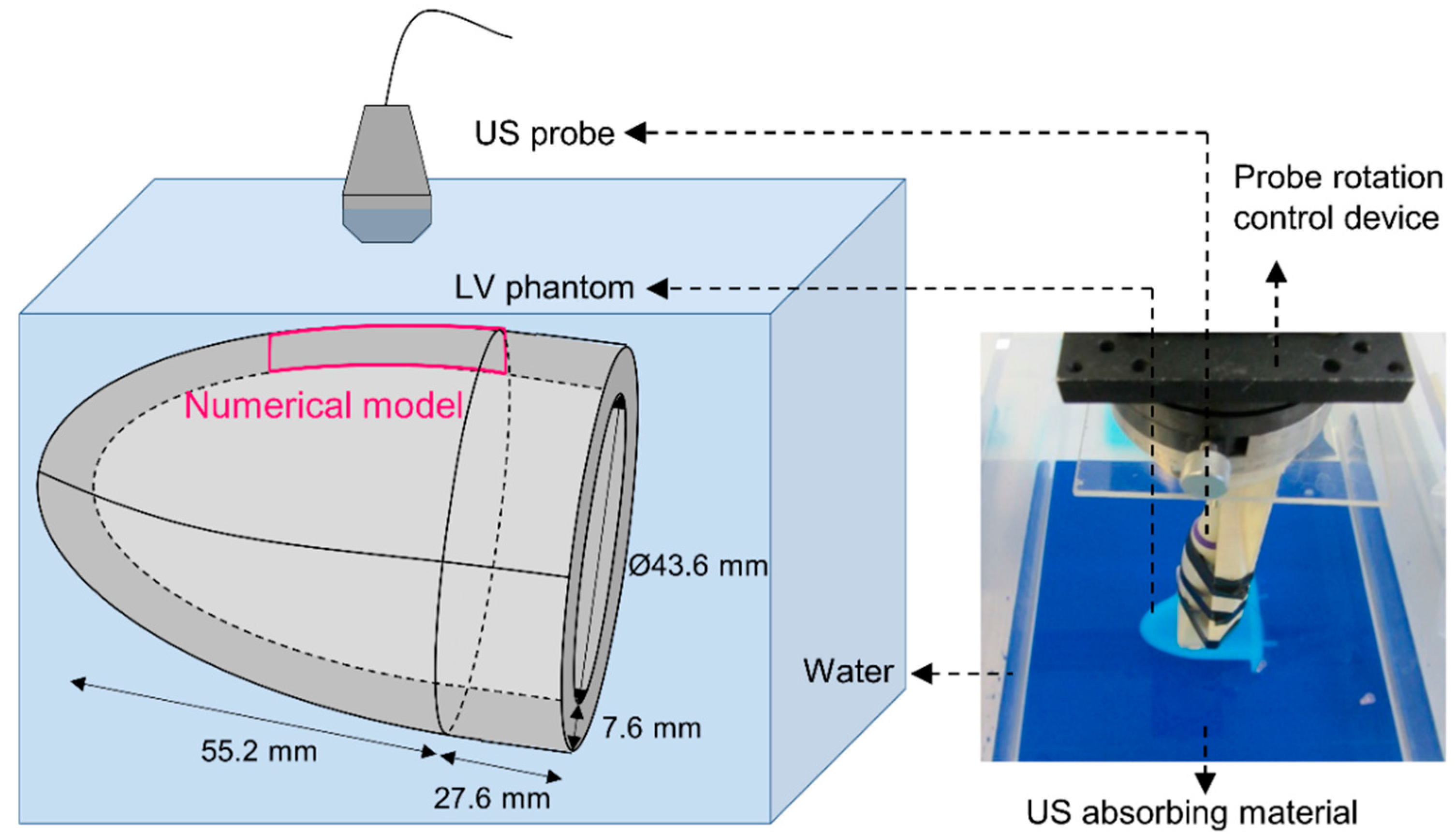
2.1. SWE Experiments

SWE acquisitions were performed on an ultrasound phantom (10% polyvinylalcohol (PVA), freeze-thawed once) of the mimicking pediatric left ventricular geometry as illustrated in Figure 1. Further details on this phantom can be found in a recent publication from our group [23]. Shear waves were generated and imaged by a SL15-4 linear transducer with 256 elements, a pitch of 200 μm and an elevation focus of ~30 mm, connected to the Aixplorer system (SuperSonic Imagine, Aix-en-Provence, France). We considered two SWE acquisitions, one with single plane wave emissions (0°) and the second with coherent plane wave compounding (−2°, 0°, 2°) [10], in which the single plane waves are emitted at a pulse repetition frequency (PRF) of 6.9 kHz for both acquisitions. All other pushing and imaging parameters for both SWE acquisitions are listed in

Table 1. In vitro imaging parameters.

	Parameters	Values
Pushing sequence	Push frequency f0	8 MHz
	F-number	2.5
	Apodization	-
	Push duration	250 µs
Imaging sequence	Number of cycles	2
	Emission frequency	8 MHz
	Pulse repetition frequency (PRF)	6.9 kHz
	Imaging depth	40 mm
	F-number on transmit	-
	Transmit apodization	-
	F-number on receive	1.2
	Receive apodization	Hanning
	Receive bandwidth	60%

. The Aixplorer system provided us beamformed in-phase and quadrature-demodulated (IQ) signals with a fast time sampling rate of 32 MHz.

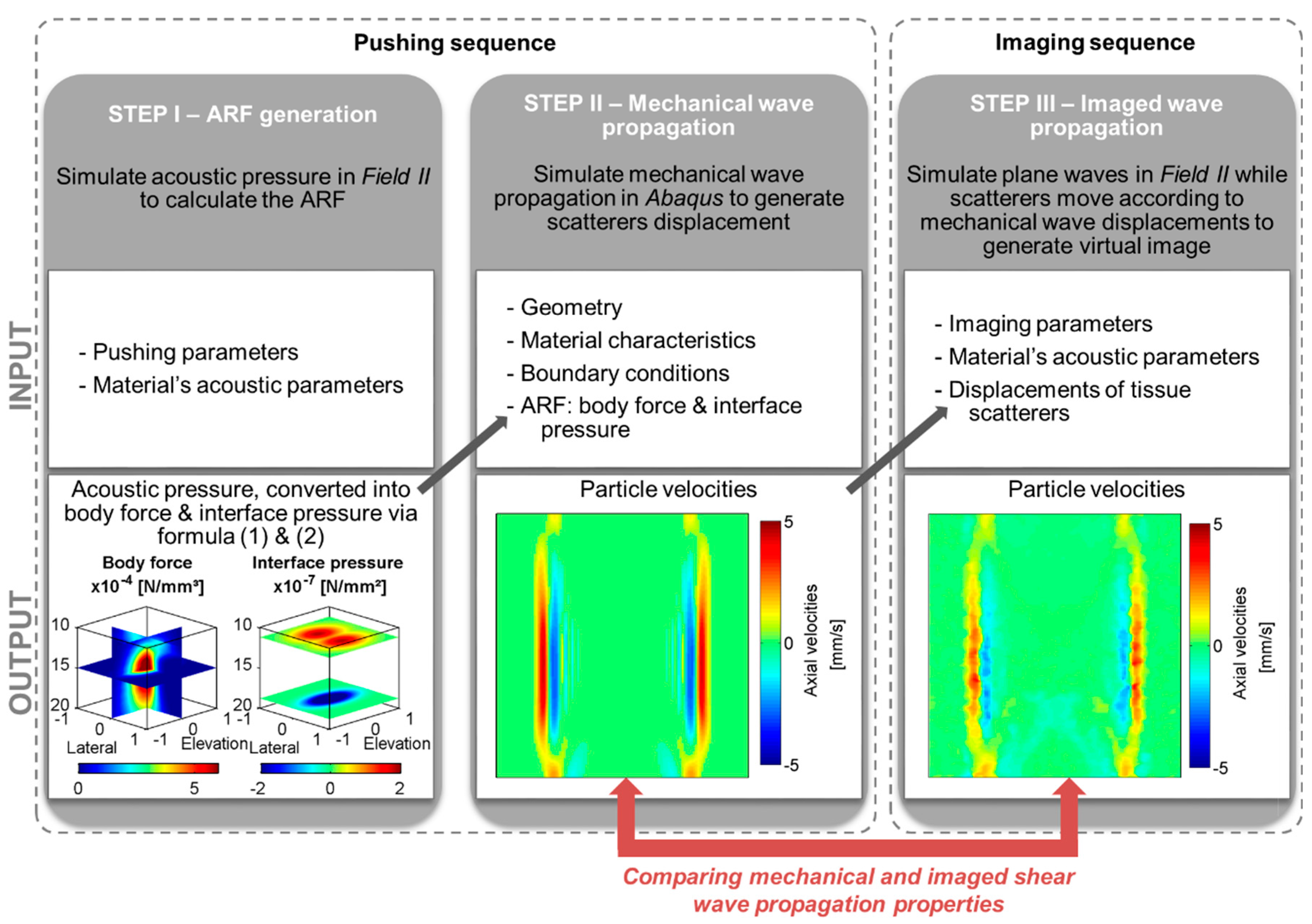
2.2. SWE Multiphysics Model

Concordant with an actual SWE measurement, the SWE model also splits the SWE acquisition into a pushing and an imaging sequence. This multiphysics platform contains three modeling parts, i.e., modeling of the acoustic radiation force (ARF), the shear wave propagation and the ultrafast imaging acquisition. The first two modeling parts compose the pushing sequence, whereas the third modeling part represents the imaging sequence (see Figure 2). These models need to be run consecutively as the output of the first model is used as input for the second model and likewise for the second and third model, as indicated by the arrows in Figure 2. The first and the third part of the multiphysics platform model the ultrasound physics through Field II [24,25], whereas the second modeling part simulates the wave mechanics in the finite element software Abaqus (Abaqus Inc., Providence, RI, USA). The modeling methodology for the pushing and imaging sequence is concisely described below. The reader is referred to [23] for further details about the pushing sequence, comprising the first two modeling parts.

2.2.1. Pushing Sequence

The pushing sequence in the numerical model consists of two steps: ARF generation and mechanical wave propagation (Figure 2). For the first step, the ARF applied on the PVA phantom is numerically mimicked by a volume force in combination with an interface pressure. Both types of loading act on the PVA phantom in the focal zone of the probe, extending ~2 mm from the probe’s center point in the lateral and elevation direction. The volume force acts throughout the complete thickness of the PVA phantom in this focal region, whereas the interface pressure is only active on the interfaces between phantom and water. Volume force $b$ and interface pressure $\pi$ are calculated based on the time-averaged acoustic intensity $I$, of which its spatial distribution is derived by simulating acoustic probe pressures mimicking the push sequence (see Table 1) with Field II and its magnitude is scaled to 1500 W/cm² [26], as follows [21,27]:

$$b=\frac{2\alpha I}{\rho c_L},$$

(1)

$$\pi =\frac{I}{c_1}\left(1+R-\left(1-R\right)\frac{c_1}{c_2}\right),$$

(2)

where $\alpha$ is the attenuation coefficient [dB/cm/MHz], $\rho$ the density of PVA [kg/m³], $c_L$ the longitudinal wave speed of PVA [m/s], $R={\left(\frac{Z_2-Z_1}{Z_2+Z_1}\right)}^2$ the energetic reflection coefficient [-], $Z_1$ and $Z_2$ the acoustic impedances ($Z_i={\rho }_i{c}_i$) [Pa∙s/m³], and $c_1$ and $c_2$ the speeds of sound in media 1 and 2 [m/s]. Material characteristics of the modeled water and PVA can be found in

Table 2. Material characteristics of water and polyvinylalcohol (PVA).

	Characteristics	Value
Water	Density $\rho$	1000 kg/m³
	Speed of sound $c_L$ [29]	1480 m/s
	Bulk modulus $K$ [29]	2200 MPa
PVA	Density $\rho$	1045.5 kg/m³
	Speed of sound $c_L$	1568 m/s
	Young’s Modulus $E$	73.0 kPa
	Attenuation coefficient $\alpha$ [30]	0.4 dB/cm/MHz
	Coefficient of Poisson $\nu$ [20]	0.49999
	Normalized shear modulus $g_1$	4.04 × 10−3
	Relaxation time ${\tau }_1$	99.8 × 10−6 s
	Normalized shear modulus $g_2$	7.04 × 10−2
	Relaxation time ${\tau }_2$	77.9 s

. The PVA’s Young’s modulus and viscoelastic behavior were mechanically determined on a uniaxial tensile testing machine (Instron 5944, Norwood, MA, USA), whereas its density and speed of sound were measured using the principle of Archimedes [28] and an oscilloscope respectively (for more details on all measurements, we refer to [23]). The resulting spatial distribution of the volume force in the axial-lateral plane is shown in the bottom-left panel of Figure 2. Both loads are imposed for 250 µs in the numerical model.

For the actual mechanical wave simulation (step II in Figure 2), the PVA phantom was modeled as one half of an ellipsoidal-shaped disk with a lateral and elevational length of 27.8 mm and 16.0 mm respectively, taking the symmetry of the imaging plane into account. For reasons of computational efficiency, we considered only half the width of the transducer in the model, and modeled structural infinite elements at the edges of the defined domain. This PVA model was meshed with 8-noded brick elements with reduced integration, leading to 355,680 elements in total. The water below and above the phantom is represented by two layers of 8-noded hexahedral acoustic elements, each with a thickness of 3.8 mm and 79,684 elements. Mechanical displacements of the PVA phantom were coupled to acoustic pressures in the water layer through a tie-constraint. The other surfaces of the modeled water were modeled to be infinite. The PVA was modeled as a viscoelastic material by assuming a 2-term Prony series model with normalized shear moduli $g_i$ and relaxation times ${\tau }_i$ as mentioned in Table 2, which are derived from a uniaxial mechanical relaxation test stretching the PVA material at 5% strain for 10 s [23]. It should be noted that the modeled viscoelasticity has a negligible influence on shear wave propagation characteristics, indicating that the actual and modeled PVA phantom have very low viscosity [23]. The water was defined as an acoustic medium in the model with bulk modulus $K$ and density $\rho$ as tabulated in Table 2. More details about mesh geometry, boundary conditions, material characteristics and loading can be found in [23].

The dynamic equations of motion of this numerical problem were solved by the Abaqus explicit solver and the particle velocities were extracted at a sampling rate of 40 kHz for further analysis. The wave propagation resulting from these simulations is called ‘mechanical shear wave propagation’ throughout this work (see Figure 2).

2.2.2. Imaging Sequence

The imaging sequence simulation in the multiphysics approach is illustrated in step 3 (Figure 2). The basis of the ultrasound simulation is Field II, in which tissue is represented by a collection of random point scatterers reflecting the ultrasonic waves emitted by the modeled probe. For each emitted beam, the scatterer’s position is updated based on the CSM extracted displacement fields, utilizing first a temporal interpolation from the CSM timescale to US timescale and subsequently spatial interpolation from CSM mesh grid to US scatterer grid. In order to obtain a proper random distribution of point scatterers within our numerical phantom, we used an algorithm based on the open-source software Visualization ToolKit (VTK) [31]. This algorithm first generates randomly distributed scatterers in a box surrounding the phantom’s geometry and then removes the abundant scatterers outside the actual geometry based on geometric criteria of the scatterers relative to the phantom’s surface [32]. Approximately 10 scatterers per resolution cell (with its size calculated based on receive F-number, transmit frequency and pulse length) were considered to ensure a Gaussian-distributed RF signal [33].

To mimic our SWE experiments (see Section 2.1), two ultrafast imaging settings were simulated, one with and one without coherent plane wave compounding, using the same probe parameters as mentioned in Table 1. However, the virtual transducer’s size was reduced to 128 piezoelectric elements to decrease computational time. For the same reason, the number of simulated frames was limited to 27 and 9 for the single and compounded Plane Wave Imaging (PWI) acquisition, respectively. For the estimation of the scatterer displacement during these simulations, the displacement information of the same CSM simulation was used since the pushing parameters or location did not change throughout the experiments (see Table 1). In our simulation setup, each transducer element was divided into four rectangular mathematical elements in the elevational direction to ensure a far-field approximation of the spatial impulse response. Channel data were acquired at a fast time sampling rate of 100 MHz, IQ-demodulated to 32 MHz and subsequently delay-and-sum beamformed with parameters mentioned in Table 1 using an in-house developed code from the Norwegian University of Science and Technology (NTNU). The obtained wave propagation from these simulations is termed ‘virtual imaged shear wave propagation’ throughout this work (see Figure 2).

2.3. Post-Processing

The data acquired from the SWE experiments and the SWE multiphysics model were both processed as described below to obtain the axial particle velocities as a function of time and space and the shear modulus estimate.

2.3.1. Axial Velocity Estimation

Axial velocities ${\widehat{v}}_z$ were obtained by applying the autocorrelation technique on the IQ-data as follows [34,35]:

$${\widehat{v}}_z=\frac{c_L\left(\frac{PRF}{n_T}\right)}{4\pi f_0}\angle {\widehat{R}}_x\left(1\right)$$

(3)

where $\angle {\widehat{R}}_x\left(1\right)$ represents the phase angle of the autocorrelation function of lag one which is estimated from the received signal sequence, and $n_T$ the number of transmit beams to obtain one image. The axial velocity estimate was further improved by spatial averaging the autocorrelation estimate over an area of approximately 0.6 × 0.6 mm both in simulations and in vitro.

Note that this post-processing step is not applied on the mechanical shear wave simulations, as these immediately provide access to all components of the particle velocities in the 3D spatial domain. Additionally, the mechanical wave simulations have a slow time sampling rate of 40 kHz, whereas the sampling rate of the real and virtual SWE imaging measurements depends on the acquisition, i.e., 6.9 kHz for single plane wave emissions and 2.3 kHz for plane wave compounding.

2.3.2. Shear Modulus Estimation

As our previous work [23] has shown that dispersive shear wave propagation patterns arose in the studied setting due to geometry, two different shear modulus estimation techniques were applied on the mechanical and (real and virtual) imaged wave propagation, i.e., a time-of-flight (TOF) method—implemented in commercial SWE systems and used for non-dispersive media—and a phase velocity analysis—used for dispersive media. The real and virtual imaging acquisitions were pre-processed by averaging the axial velocities over 0.6 mm axial depth and temporally up-sampling the slow time domain by a factor 10.

For the TOF method, the shear wave’s position was tracked by searching the maximal axial velocity for every lateral spatial location as a function of time and fitting a linear model to estimate the shear wave velocity (goodness of fit should be equal to or larger than 0.95) [23,36]. In general, to make the most complete use of the measured data and to increase the reliability of the fit, axial velocity data acquired from all probe elements should be taken into account during this linear fitting procedure. This is true for large isotropic homogeneous elastic media, but usually data from the probe’s edge elements is discarded due to low signal-to-noise ratio and/or high attenuation of the propagating shear wave in the measurement. Even though the studied PVA setting is isotropic, homogeneous and low viscous, the left ventricular geometry induces dispersive shear wave features in the SWE-acquisitions which affect the tracked shear wave’s position as a function of time. To investigate the effect of this observation on the results of the TOF method, we altered the number of data points taken into account during the TOF fitting procedure: the shear wave speed was estimated by rejecting 5 and 20 data points from the probe’s edge elements for each shear wave. The shear modulus $\mu$ can then be derived from this wave speed $c_T$ by assuming an isotropic bulky elastic material with density $\rho$ and applying the following formula:

$$\mu =\rho c_T^2$$

(4)

For the phase velocity analysis, measured or simulated dispersion characteristics were derived by taking the 2D Fast Fourier Transform (FFT) of the axial velocity wave propagation pattern as a function of lateral space and slow time at a specific depth [37]. Subsequently, the wavenumber $k$ with the maximal Fourier energy is tracked at each frequency f in order to identify the main excited mode. Phase velocity $c_{\phi }$ as a function of frequency $f$ is found through $c_{\phi }=\left(2\pi f\right)/k$. The shear modulus is then estimated by fitting a theoretical model in a least squares manner to the obtained dispersion curve. Neglecting the ventricular curvature [38] and PVA’s viscoelasticity, and assuming that the main excited mode is the first antisymmetric mode (A0) [17], we minimized the difference between the theoretical A0 dispersion curve of a plate in water and the extracted dispersion characteristics over a frequency range spanning from 0.2 kHz up to maximally 2 kHz, dependent on the considered acquisition [37,39]. Only fits giving a standard deviation less than 0.6 kPa for the shear modulus estimate were considered.

Both procedures were repeated for multiple depths across the phantom’s thickness (n = 10). For further details on both shear modulus estimation techniques, we refer to [23].

3. Results

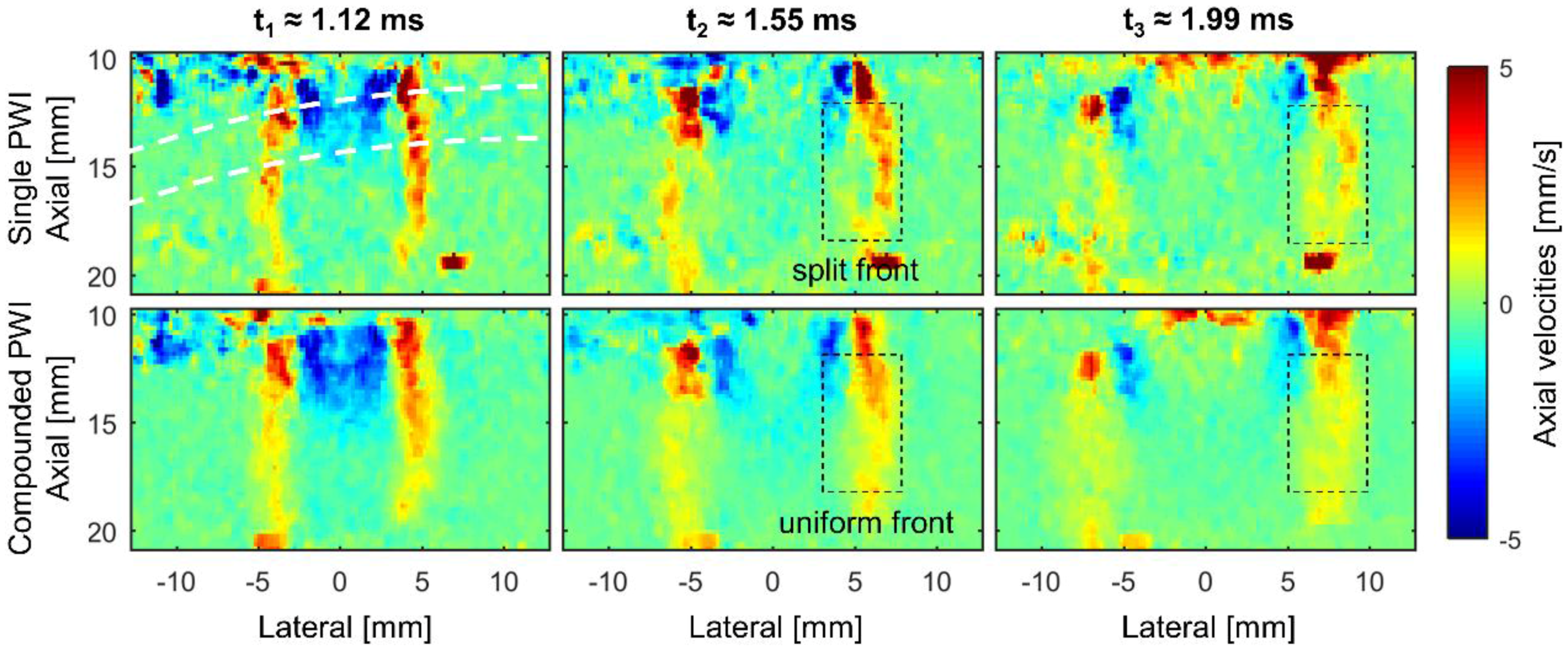
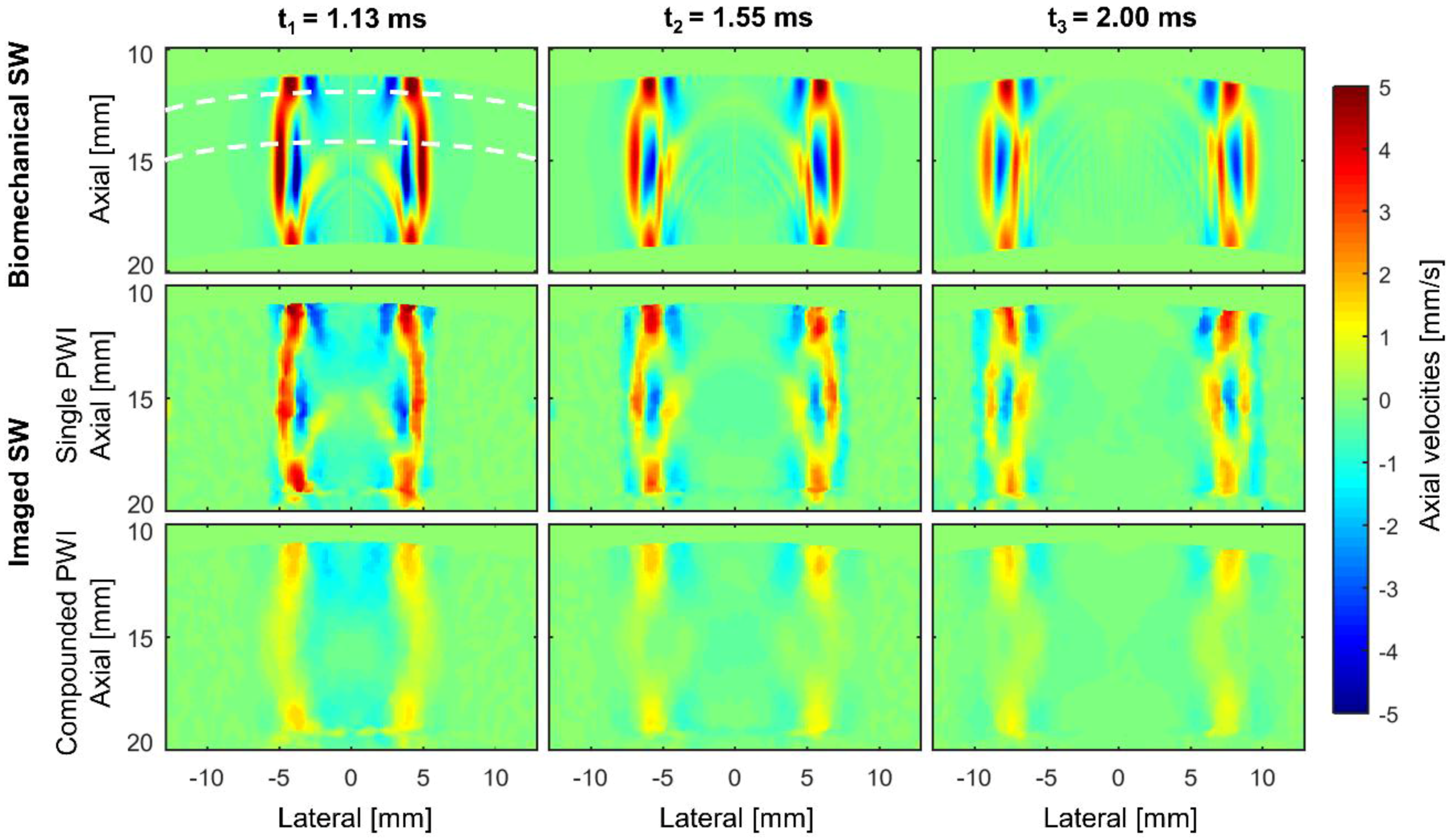
3.1. Analyzing the Shear Wave’s Characteristics in the Time Domain

To study the shear wave’s temporal characteristics, we examined its magnitude and shape throughout time by visualizing the axial velocities at three different time points. The resulting shear wave propagation of the experimentally measured SWE acquisitions with and without compounding are compared in Figure 3. Immediately, we observe a different shear wave propagation pattern: the shear wave front, represented by the downward axial velocities, is split into two for the single plane wave images whereas one uniform wave front is present for the compounded images. Furthermore, the wave front is also broader along the lateral direction when including compounding. Next to these differences in shear wave shape, we also observe a lower shear wave magnitude (maximal axial velocity amplitude at a certain time point can be up to 3 mm/s smaller) for the compounded images.

The imaged and biomechanical shear wave propagation for the simulations are depicted in Figure 4. For the biomechanical simulation (first row in Figure 4), we observe again a split in shear wave front during wave propagation, which is well captured in the virtual single plane wave images (second row in Figure 4), but less visible in the virtual compounded images (third row in Figure 4). Furthermore, the shear wave front is apparently broader in the imaging simulations compared to the biomechanical simulation. Additionally, the simulated axial velocity patterns of the virtual images show a clear decrease in tissue velocity magnitude (~23.0% for single PWI and ~69.4% for compounded PWI at the top of the phantom compared to the biomechanics simulation).

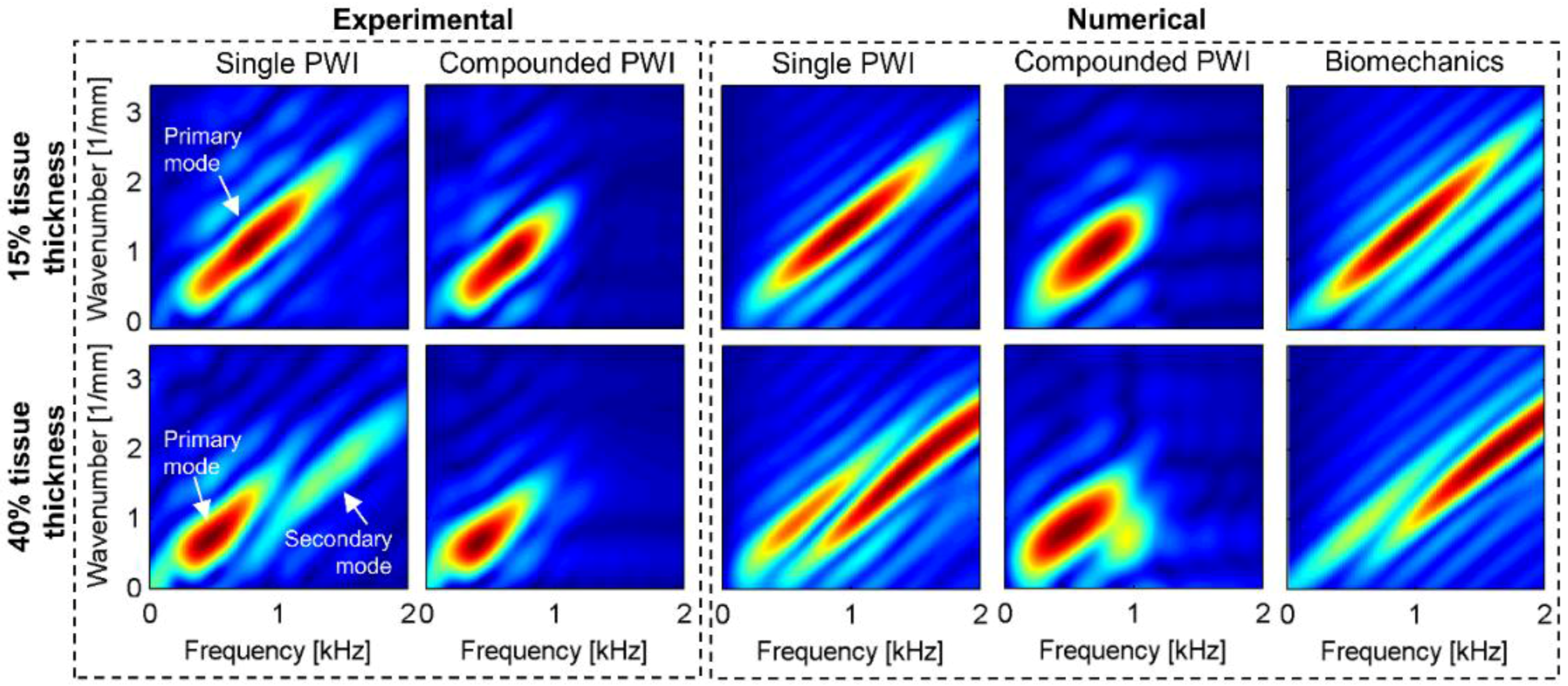
3.2. Analyzing the Shear Wave’s Characteristics in the Frequency Domain

The shear wave’s frequency features were studied by taking the 2D FFT of the axial velocity map in time and lateral space (see Methods section) at 15% and 40% tissue thickness, representing two different shear wave propagation paths as indicated by the white dotted lines in Figure 3 and Figure 4. The Fourier energy magnitudes of both simulations and measurements are mentioned in

Table 3. Tabulation of the magnitude of the maximal Fourier energy amplitude in Figure 5 [mm/s/Hz].

Acquisition		15% Tissue Thickness	40% Tissue Thickness
Experimental
	Single PWI	6.52	3.42
	Compounded PWI	1.68	1.26
Numerical
	Single PWI	5.13	3.45
	Compounded PWI	0.64	0.33
	Biomechanics	33.37	31.91

. Observations concerning mode(s) excitation, Fourier energy magnitude and frequency content in the Fourier spectra are consecutively discussed below.

3.2.1. Mode(s) Excitation

For experimental single PWI (first column of Figure 5), we observed that mainly one mode was excited at the shallow tissue depth, whereas two modes were excited for deeper tissue regions. The mode excited on lower frequencies is designated with the term ‘primary mode’, whereas the other mode is defined as ‘secondary mode’. This primary mode is the one that will be tracked and fitted to the theoretical A0-mode in the phase velocity analysis to estimate shear stiffness. Applying compounding in the experiment led to one visible excited mode in the spectra of both tissue depths, as can be seen in the second column of Figure 5. For the simulations (third, fourth and fifth columns of Figure 5), we see one excited mode for 15% tissue thickness, and two excited modes for 40% tissue thickness, independent of the application of the compounding technique.

3.2.2. Fourier Energy Magnitude

For the applied experiments, coherent compounding decreased the maximal Fourier energy magnitude with a factor of 3.9 for 15% tissue depth and 2.7 for 40% tissue thickness (see Table 3). A similar observation was made for the simulations: compounding reduced the maximal Fourier energy magnitude by factors of 8.0 and 10.5 for 15% and 40% tissue thickness respectively. Furthermore, when comparing the virtual single PWI to the biomechanics simulation, an additional decrease by factors of 6.5 and 9.2 was noticed for the two considered tissue depths. Next to these dissimilarities in maximal Fourier energy magnitude, the relative energy magnitude of secondary to primary mode for the deeper tissue region also differed (see Figure 5). This proportion was 0.5 for the experimental single PWI. For the simulations, this ratio shifted from 1.7 for the virtual biomechanics to 1.3 for single PWI and 0.6 for compounded PWI.

3.2.3. Frequency Content

The bandwidth of the Fourier spectra was about 2.0 kHz for the experimental single PWI and 1.0 kHz for the compounded acquisition (Figure 5), at both tissue depths. On the other hand, the bandwidth of the simulated Fourier spectra of the single PWI acquisition was around 2.0 kHz for 15% tissue thickness, and 3.0 kHz for 40% tissue thickness. When compounding was applied in the simulations, the maximal excited frequency was reduced to nearly 1.0 kHz for both tissue depths. However, the bandwidth of the biomechanical Fourier spectra of both virtual imaging acquisitions was about 2.0 kHz and 3.5 kHz for 15% and 40% tissue thickness respectively.

The frequency content of the detected signal was further changed when compounding was used: the frequency with maximal Fourier energy content shifted from 0.69 kHz to 0.79 kHz for 15% tissue thickness and from 0.42 kHz to 0.47 kHz for 40% tissue thickness. For the virtual single PWI, the maximal Fourier energy was reached at 0.98 kHz for 15% tissue thickness and 1.4 kHz for 40% tissue thickness. Coherent compounding in the simulations downshifted these frequencies to about 0.50 kHz for both tissue regions. The frequencies with highest Fourier energy content in the biomechanics simulation were 0.93 kHz and 1.70 kHz for 15% and 40% tissue thickness respectively.

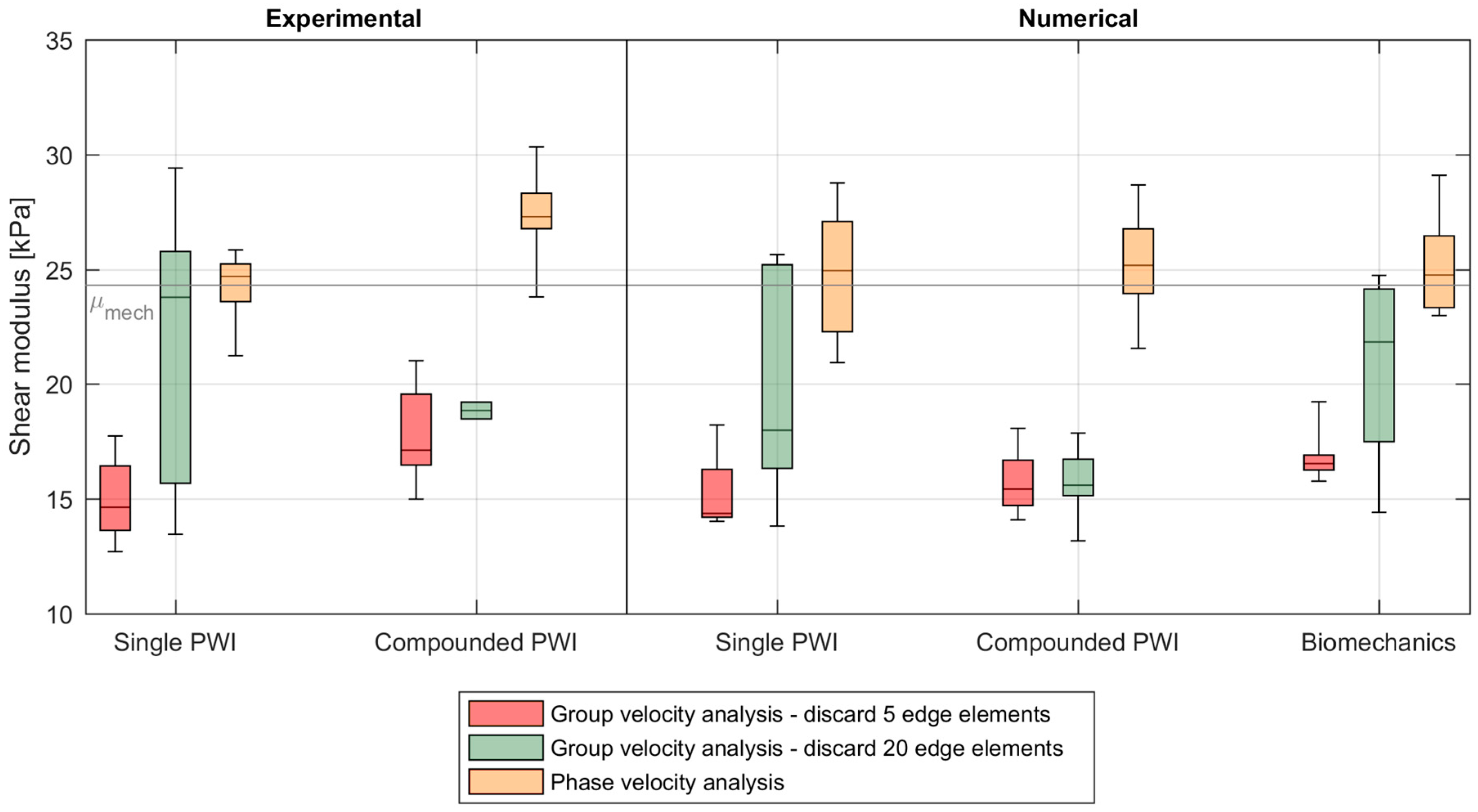
3.3. Shear Wave Speed Analysis

The quantitative analysis of shear wave observations consisted of shear modulus estimation based on group and phase velocity analysis for real and virtual SWE acquisitions, as visualized in Figure 6. For the measurements, the group velocity analysis provided median shear stiffness values of 14.6 kPa and 17.1 kPa for single and compounded PWI respectively, when discarding data of 5 edge elements for each shear wave during shear modulus estimation. These estimations increased to 23.8 kPa and 18.8 kPa when 15 more data points were not considered during the fitting procedure for each shear wave. Phase velocity analysis gave median values of 24.7 kPa and 27.3 kPa for the measurements. For single PWI, the stiffness range of TOF-estimations when taking less data points into account during fitting (15.9 kPa) was remarkably higher than for other stiffness estimation methods (5.0 kPa and 4.6 kPa for group and phase speed analysis respectively). Actual PVA stiffness was mechanically determined at 24.3 ± 0.6 kPa.

For the virtual imaging acquisitions, the group velocity-based method estimated median stiffness at 14.4 kPa and 15.4 kPa for single and compounded PWI respectively. When discarding data from 20 edge probe elements, TOF stiffness estimations increased to 18.0 kPa and 15.6 kPa. Phase velocity analysis provided, for both imaging simulations, higher estimates of median shear stiffness, i.e., 24.9 kPa and 25.2 kPa for single and compounded PWI respectively. As for the experiments, the largest spread in stiffness estimation across depth (11.8 kPa) was obtained for single PWI when applying the group velocity analysis and discarding data from 20 probe elements. For the biomechanics simulations, median shear stiffness of 16.5 kPa, 21.8 kPa and 24.7 kPa were obtained for group velocity (discarding 5 data points), group velocity (discarding 20 data points) and phase velocity analysis respectively. Again, the depth-dependency of stiffness estimations was the largest for the group speed method taking less data points into account during fitting (10.3 kPa).

4. Discussion

4.1. Multiphysics Modeling

In this work, a SWE multiphysics modeling approach incorporating the biomechanics and imaging physics of the shear wave propagation problem was presented, providing valuable insights into how the ultrafast US sequence and signal processing affects the true shear wave’s characteristics in the time and frequency domain, and the subsequent shear modulus characterization. Furthermore, a modeling approach offers the benefits of full flexibility at the level of the tissue mechanics (tissue geometry, material properties and tissue surrounding) and ultrasound physics (ARF configuration, imaging settings and processing techniques). This approach was applied to a low-viscous pediatric ventricular phantom model, displaying clear shear wave dispersion as can be seen from the frequency-dependent phase velocity in the Fourier spectra and the split shear wave front in the temporal shear wave pattern for both experiment and biomechanics model [23]. The ventricular geometry was mainly the cause of the observed dispersion, as incorporating the measured viscoelastic material properties in the model did not significantly alter the shear wave characteristics (see [23] for details). A similar multiphysics approach has already been used by Palmeri et al. [40] to study jitter errors and displacement underestimation in unbounded media, also in combination with experiments. Another study [41] used these same tools to investigate how parameters related to shear wave excitation and tracking affected the quality of shear wave speed images. However, both studies mimicked a different elastography technique, called Acoustic Radiation Force Imaging (ARFI), which employs conventional line-by-line scanning instead of plane wave imaging to visualize the shear wave propagation.

In general, the multiphysics model was capable of reproducing the experimental results (see Figure 3, Figure 4, Figure 5 and Figure 6), indicating that the simulated biomechanical ground truth is a good representation of the actual shear wave physics occurring in the PVA phantom. However, there were also some discrepancies in shear wave visualization and characterization. For the shear wave’s characteristics in the time and frequency domain, we firstly noticed a different axial velocity magnitude (see Figure 3 and Figure 4) and Fourier energy amplitude (see Table 3) as a result of scaling the time-averaged acoustic intensity to 1500 W/cm² when calculating the numerical ARF. For the virtual compounded acquisition, there was the additional effect of large shear wave travel in between ultrasound frames in combination with the presence of high relaxation velocities (blue in Figure 4) in the biomechanical simulation, indicating that compounding in the simulation reduces the downward velocities (red in Figure 4) more than in the experiment. Secondly, there were also differences in the temporal axial velocity pattern (e.g., larger relaxation peak at the center of the phantom for the simulations) and frequency spectra (e.g., more secondary mode excitation at 40% tissue thickness in the simulations). This can potentially be attributed to: (i) the manner of shear wave excitation in the model, i.e., applying a time-averaged body force and interface pressure instead of modeling the longitudinal wave propagation in the focused US beam, including reflection and attenuation, (ii) the difference in location of the actual and virtual SWE acquisitions, and (iii) the unknown experimental dead time between the pushing and imaging sequence. It should also be kept in mind that the beamforming process for experiment and simulation was performed with different infrastructure, i.e., the Aixplorer system and the NTNU in-house developed beamformer, respectively. Next to these dissimilarities in shear wave pattern in time and frequency, there were also inconsistencies in shear modulus estimation (Figure 6). These discrepancies are partly due to the same factors, as explained above, influencing shear wave propagation patterns and thus also stiffness characterization. Additionally, the simulations are noise-free, allowing more reliable shear stiffness estimates for every shear wave propagation path across depth compared to the experiments. Another potential cause explaining the stiffness discrepancy between experiment and simulation is a wrongly modeled material stiffness (based on uniaxial mechanical testing), as the mechanical properties of the PVA phantom could alter in the time difference between mechanical testing and SWE experiment.

4.2. Effect of Ultrafast Imaging on SWE in the Studied Left Ventricular Model

We studied the effect of ultrafast imaging on SWE by comparing shear wave visualization and characterization obtained from US and CSM simulations of our left ventricular phantom model. When analyzing the temporal shear wave patterns of all simulations in Figure 4, a clear broadening of the shear wave front and underestimation of axial velocities is noticeable for both imaging acquisitions. A similar negative velocity bias was also recently reported when using coherent plane wave compounding for Doppler imaging [42]. Furthermore, the plane wave compounded images revealed a shear wave pattern different than the single plane wave images: the split shear wave front, clearly visible in the single plane wave acquisition, was less observable in the compounded images (Figure 4). Furthermore, the experimental compounded images in Figure 3 showed a completely merged wave front instead of the split wave front as observed in the single plane wave images. Even though this observation was less clearly noticeable in the simulations (due to the presence of a larger relaxation peak in between the split wave front compared to the measurements, as mentioned in Section 4.1), the multiphysics model still demonstrated that these observed differences in temporal characteristics of the shear wave are mainly attributed to the chosen imaging parameters, as both virtual imaging acquisitions were derived from the same true mechanical wave propagation (see Figure 4). We also investigated the subsequent changes in the shear wave’s frequency characteristics, which showed that the detected excited frequencies, amplitudes and modes did not necessarily correspond to the ones excited in the biomechanical model. Indeed, the biomechanical frequency spectra are solely dependent on the model characteristics and the ARF properties [43], whereas the imaged spectra are also affected by plane wave imaging, acting as a low-pass filter, and by image processing techniques such as pixel averaging and slow time up-sampling.

Next to this qualitative investigation, we also quantitatively studied the effect of ultrafast imaging on the performance of SWE by comparing the SWE-derived shear modulus for both US and CSM simulations (see Figure 6). This study showed that ultrafast imaging had mainly an effect on stiffness characterization through the group speed method: single and compounded PWI simulations led to median stiffness underestimations of −2.2 kPa (−4.0 kPa when discarding 20 data points) and −1.1 kPa (−6.2 kPa when discarding 20 data points) respectively compared to the SWE-derived stiffness estimates from the biomechanical simulations. Additionally, the results of the TOF method when discarding 20 edge elements were very depth-dependent for the single PWI simulation. This was also observed for the experiments in Figure 6. This large dissimilarity in depth-dependency of the stiffness estimates is due to a difference in meaning of the fitted linear relationship in the TOF method when discarding more or less data points for the single PWI acquisition. When 20 data points are discarded during the fitting procedure, the fitted linear relationship represents the true non-shifted shear wave position throughout time which varies a lot across depth, whereas it depicts an averaged shear wave position in time when only 5 data points are discarded (Figure S1). The latter corresponds to the TOF shear wave characterization with compounded PWI (as can be seen in Figure 6 and Figure S1), as the compounded images already visualize the averaged shear wave behavior. Nevertheless, the shear modulus estimates are depth-dependent for all applied material characterization methods, as can be seen in the spread of the boxplots in Figure 6. For the group velocity analysis (discarding 5 data points), this is mainly due to the difference in the shear wave propagation pattern at the upper and lower boundaries of the phantom (±0–25% and ±75–100% depth) compared to the middle segment of the phantom (±25–75% depth), as visible in Figure S1. This group speed-derived stiffness difference between the boundaries and center of a tissue-mimicking medium was experimentally studied by Mercado et al. [44], in which they identified the presence of Scholte surface waves at the fluid–solid interface as the primary reason for this discrepancy. For the phase velocity analysis, the cause of the depth-dependency of the stiffness estimates is less straightforward, as the extracted frequency characteristics of the primary mode across depth were very similar (see Figure 5). However, as also shown in [23], characterizing deeper shear waves via the phase velocity analysis is more challenging as their 2D FFT energy content is smaller (fewer data points to fit) and their velocity amplitude is lower (lower signal-to-noise ratio), leading to less reliable shear modulus estimates.

Phase velocity analysis provided a more robust and correct estimate for both the biomechanics and imaging simulations, as spectral characteristics of the tracked primary mode (fitted to the theoretical A0-mode) for all acquisitions are very similar, as shown in Figure 5. Furthermore, for both experiment and simulation, the true tissue stiffness was underestimated by the TOF method, independent of the number of considered data points, whereas phase velocity analysis provided a better estimate of the mechanically determined stiffness. This is in accordance with our previous findings of experimental work on the same ventricular model in which we only applied single PWI [23]. Nevertheless, if the stiffness estimation technique is chosen based on observed shear wave physics (i.e., TOF method for compounded images visualizing almost no dispersion and phase velocity analysis for single plane wave images depicting dispersion), differences of minimally 5.9 kPa and 9.3 kPa are obtained for measurements and simulations, respectively. This is about 25% of the value of the actual shear modulus, and non-negligible. Therefore, when studying low viscous settings evoking guided wave dispersion due to geometry, one should be cautious when selecting a tissue characterization method based on the observed shear wave pattern as this might be affected by the applied imaging set-up. In these cases, it might be relevant to also study phase velocity next to group velocity.

It should be noted that the primary objective of this work was not to compare the performance of single and compounded PWI, as this requires (i) the study of multiple configurations and material models, (ii) the use of more complex SWE-based material characterization and (iii) the inclusion of noise in the numerical models. However, this work shows the potential of computational modeling in identifying potential pitfalls in shear wave visualization and characterization with SWE, demonstrated through a case study of an idealized SWE setting with little amount of noise (as shown by the good correspondence between experiment and simulation). Future research should focus on applying the current modeling technique to different settings to further study the performance of single and compounded PWI.

4.3. Recommendations and Impact for Other Applications

The dispersive shear wave propagation pattern studied here is inherently linked to the considered setting, i.e., a left ventricular low viscous phantom with pediatric geometry. We focused on the isolated effect of guided wave dispersion due to geometry, and therefore, the formulated conclusions cannot simply be extrapolated to actual tissue settings as dispersion in tissues can be caused by a combination of varying factors such as geometry, viscosity and non-homogeneous (potentially anisotropic) material characteristics. This is among other things noticeable in the excited frequency range of the studied shear wave (up to 2 kHz), which is much larger than the conventional 1 kHz shear wave frequency spectra reported in real tissue settings due to tissue’s high shear viscosity [17]. Additionally, the observed shear wave fronts were quite isotropic in all directions of the shear wave paths in 2D, whereas these will become guided along the fiber orientation in anisotropic tissue [45,46]. These true tissue characteristics demand more advanced tissue characterization algorithms as now (i) an isotropic bulky elastic material is assumed in the group speed analysis in order to apply Formula (4), and (ii) a theoretical dispersion curve of an isotropic homogeneous elastic plate in water is used as fitting ground truth in the phase speed analysis. Therefore, complementary research is necessary to investigate how the formulated conclusions concerning shear wave visualization and characterization are translated to actual tissue settings in vivo, particularly when assessing the effect of compounding.

Despite these dissimilarities between shear wave physics in the phantom-model and actual tissue, the multiphysics model of the presented case study allowed the assessment of the effect of ultrafast imaging on shear wave visualization and characterization from a mechanical point of view, as described in the previous section. Furthermore, this study showed that the number of compounding angles (i.e., the factor with which the frame rate is reduced) should be chosen taking the maximal reachable PRF (linked to imaged depth and technical capabilities of the ultrasound system), the wave propagation speed of the investigated material (related to its mechanical properties) and the bandwidth of the imaged phenomenon (related to different absorption mechanisms such as viscosity) into account. The resulting compounded frame rate should be sufficiently high to obtain an accurate representation of the mechanical shear wave physics, which was not the case for the studied left ventricular phantom model. Additionally, a high frame rate is also desirable from the shear wave characterization point of view, as this means a high Nyquist cut-off frequency, providing a more extensive Fourier spectrum, and thus a more reliable stiffness estimate via the phase velocity analysis.

Similar recommendations were recently published by Widman et al. [19], who studied the optimal ARF and imaging settings to maximize bandwidth for phase velocity analysis in SWE on ex vivo arterial settings. In their study on arterial stiffness estimation, they claimed that a high PRF with poorer image quality is more desirable than a lower PRF with better image quality.

5. Conclusions

In this work, we assessed the effect of ultrafast imaging on dispersive shear wave visualization and subsequent shear stiffness characterization by means of SWE experiments in combination with a multiphysics model of a LV phantom model with pediatric geometry. This model offers the advantage of giving access to the true biomechanical wave propagation, which is unknown in the SWE measurements. The multiphysics model of the idealized LV phantom revealed that the detected shear wave features in the time and frequency domain by ultrafast imaging do not necessarily depict the ARF-excited characteristics of the biomechanical model. Furthermore, application of the compounding technique in ultrafast imaging even altered the dispersion features in the temporal shear wave pattern for both experiments and simulations, leading to a stiffness underestimation of minimally 25% when choosing a group velocity-based algorithm instead of a phase velocity one. Additionally, the applied group speed material characterization method was very sensitive to the applied algorithm settings (such as the number of tracked data points) and the selected axial depth, as ultrafast imaging can alter the shear wave front location in the shear wave visualization. Therefore, it is important to keep a high frame rate during compounding in order to obtain an accurate representation of shear wave physics and the subsequently derived material stiffness. Future research should focus on investigating additional configurations with more advanced SWE-based material characterization to further generalize these conclusions. Nevertheless, this work presents a versatile and powerful simulation environment to evaluate the performance of ultrafast imaging in shear wave visualization and characterization with SWE, and to identify potential pitfalls in accurately capturing shear wave propagation.

References

1. Bercoff, J. Ultrafast Ultrasound Imaging. In Ultrasound Imaging—Medical Applications; Minin, P.O., Ed.; Intech: Rijeka, Croatia, 2011. [Google Scholar]
2. Tanter, M.; Fink, M. Ultrafast imaging in biomedical ultrasound. IEEE Trans. Ultrason. Ferroelectr. Freq. Control 2014, 61, 102–119. [Google Scholar] [CrossRef] [PubMed]
3. Tanter, M.; Bercoff, J.; Sandrin, L.; Fink, M. Ultrafast Compound Imaging for 2-D Motion Vector Estimation: Application to Transient Elastography. IEEE Trans. Ultrason. Ferroelectr. Freq. Control 2002, 49, 1363–1374. [Google Scholar] [CrossRef] [PubMed]
4. Sandrin, L.; Tanter, M.; Catheline, S.; Fink, M. Shear Modulus Imaging with 2-D Transient Elastography. IEEE Trans. Ultrason. Ferroelectr. Freq. Control 2002, 49, 426–435. [Google Scholar] [CrossRef] [PubMed]
5. Bercoff, J.; Tanter, M.; Fink, M. Supersonic Shear Imaging: A New Technique for Soft Tissue Elasticity Mapping. IEEE Trans. Ultrason. Ferroelectr. Freq. Control 2004, 51, 396–409. [Google Scholar] [CrossRef] [PubMed]
6. Gennisson, J.L.; Deffieux, T.; Fink, M.; Tanter, M. Ultrasound elastography: Principles and techniques. Diagn. Interv. Imaging 2013, 94, 487–495. [Google Scholar] [CrossRef] [PubMed]
7. Sarvazyan, A.P.; Rudenko, O.V.; Swanson, S.D.; Fowlkes, J.B.; Emelianov, S.Y. Shear Wave Elasticity Imaging: A New Ultrasonics Technology of Medical Diagnostics. Ultrasound Med. Biol. 1998, 24, 1419–1435. [Google Scholar] [CrossRef]
8. Nightingale, K.; Soo, M.S.; Nightingale, R.; Trahey, G. Acoustic Radiation Force Impulse Imaging: In Vivo Demonstration of Clinical Feasibility. Ultrasound Med. Biol. 2002, 28, 227–235. [Google Scholar] [CrossRef]
9. Doherty, J.R.; Trahey, G.E.; Nightingale, K.R.; Palmeri, M.L. Acoustic radiation force elasticity imaging in diagnostic ultrasound. IEEE Trans. Ultrason. Ferroelectr. Freq. Control 2013, 60, 685–701. [Google Scholar] [CrossRef] [PubMed]
10. Montaldo, G.; Tanter, M.; Bercoff, J.; Benech, N.; Fink, M. Coherent Plane-Wave Compounding for Very High Frame Rate Ultrasonography and Transient Elastography. IEEE Trans. Ultrason. Ferroelectr. Freq. Control 2009, 56, 489–506. [Google Scholar] [CrossRef] [PubMed]
11. Bercoff, J.; Montaldo, G.; Loupas, T.; Savery, D.; Mézière, F.; Fink, M.; Tanter, M. Ultrafast Compound Doppler Imaging: Providing Full Blood Flow Characterization. IEEE Trans. Ultrason. Ferroelectr. Freq. Control 2011, 58, 134–147. [Google Scholar] [CrossRef] [PubMed]
12. Papadacci, C.; Pernot, M.; Couade, M.; Fink, M.; Tanter, M. High Contrast Ultrafast Imaging of the Human Heart. IEEE Trans. Ultrason. Ferroelectr. Freq. Control 2014, 61, 288–301. [Google Scholar] [CrossRef] [PubMed]
13. Couture, O.; Bannouf, S.; Montaldo, G.; Aubry, J.F.; Fink, M.; Tanter, M. Ultrafast imaging of ultrasound contrast agents. Ultrasound Med. Biol. 2009, 35, 1908–1916. [Google Scholar] [CrossRef] [PubMed]
14. Mace, E.; Montaldo, G.; Osmanski, B.F.; Cohen, I.; Fink, M.; Tanter, M. Functional ultrasound imaging of the brain: Theory and basic principles. IEEE Trans. Ultrason. Ferroelectr. Freq. Control 2013, 60, 492–506. [Google Scholar] [CrossRef] [PubMed]
15. Tanter, M.; Bercoff, J.; Athanasiou, A.; Deffieux, T.; Gennisson, J.L.; Montaldo, G.; Muller, M.; Tardivon, A.; Fink, M. Quantitative assessment of breast lesion viscoelasticity: Initial clinical results using supersonic shear imaging. Ultrasound Med. Biol. 2008, 34, 1373–1386. [Google Scholar] [CrossRef] [PubMed]
16. Ferraioli, G.; Parekh, P.; Levitov, A.B.; Filice, C. Shear wave elastography for evaluation of liver fibrosis. J. Ultrasound Med. 2014, 33, 197–203. [Google Scholar] [CrossRef] [PubMed]
17. Couade, M.; Pernot, M.; Prada, C.; Messas, E.; Emmerich, J.; Bruneval, P.; Criton, A.; Fink, M.; Tanter, M. Quantitative assessment of arterial wall biomechanical properties using shear wave imaging. Ultrasound Med. Biol. 2010, 36, 1662–1676. [Google Scholar] [CrossRef] [PubMed]
18. Nguyen, T.M.; Couade, M.; Bercoff, J.; Tanter, M. Assessment of Viscous and Elastic Properties of Sub-Wavelength Layered Soft Tissues Using Shear Wave Spectroscopy: Theoretical Framework and In Vitro Experimental Validation. IEEE Trans. Ultrason. Ferroelectr. Freq. Control 2011, 58, 2305–2315. [Google Scholar] [CrossRef] [PubMed]
19. Widman, E.; Maksuti, E.; Amador, C.; Urban, M.W.; Caidahl, K.; Larsson, M. Shear Wave Elastography Quantifies Stiffness in Ex Vivo Porcine Artery with Stiffened Arterial Region. Ultrasound Med. Biol. 2016, 42, 2423–2435. [Google Scholar] [CrossRef] [PubMed]
20. Caenen, A.; Shcherbakova, D.; Verhegghe, B.; Papadacci, C.; Pernot, M.; Segers, P.; Swillens, A. A Versatile and Experimentally Validated Finite Element Model to Assess the Accuracy of Shear Wave Elastography in a Bounded Viscoelastic Medium. IEEE Trans. Ultrason. Ferroelectr. Freq. Control 2015, 62, 439–450. [Google Scholar] [CrossRef] [PubMed]
21. Palmeri, M.L.; Sharma, A.C.; Bouchard, R.R.; Nightingale, R.W.; Nightingale, K.R. A Finite-Element Method Model of Soft Tissue Response to Impulsive Acoustic Radiation Force. IEEE Trans. Ultrason Ferroelectr. Freq. Control 2005, 52, 1699–1712. [Google Scholar] [CrossRef] [PubMed]
22. Lee, K.H.; Szajewski, B.A.; Hah, Z.; Parker, K.J.; Maniatty, A.M. Modeling shear waves through a viscoelastic medium induced by acoustic radiation force. Int. J. Numer. Methods Biomed. Eng. 2012, 28, 678–696. [Google Scholar] [CrossRef] [PubMed]
23. Caenen, A.; Pernot, M.; Shcherbakova, D.A.; Mertens, L.; Kersemans, M.; Segers, P.; Swillens, A. Investigating Shear Wave Physics in a Generic Pediatric Left Ventricular Model via In Vitro experiments and Finite Element Simulations. IEEE Trans. Ultrason. Ferroelectr. Freq. Control 2017, 64, 349–361. [Google Scholar] [CrossRef] [PubMed]
24. Jensen, J.A. Field: A Program for Simulating Ultrasound Systems. In Proceedings of the 10th Nordic-Baltic Conference on Biomedical Imaging, Tampere, Finland, 9–13 June 1996; pp. 351–353. [Google Scholar]
25. Jensen, J.A.; Svensen, N.B. Calculation of Pressure Fields from Arbitrarily Shaped, Apodized, and Excited Ultrasound Transducers. IEEE Trans. Ultrason. Ferroelectr. Freq. Control 1992, 39, 262–267. [Google Scholar] [CrossRef] [PubMed] [Green Version]
26. Nightingale, K. Acoustic Radiation Force Impulse (ARFI) Imaging: A Review. Curr. Med. Imaging Rev. 2011, 7, 328–339. [Google Scholar] [CrossRef] [PubMed]
27. Shutilov, V. Fundamental Physics of Ultrasound; CRC Press: Boca Raton, FL, USA, 1988. [Google Scholar]
28. Standard Test Methods for Density and Specific Gravity (Relative Density) of Plastics by Displacement; ASTM Standard D792-08; ASTM International: West Conshohocken, PA, USA, 2008.
29. Kamopp, D.C.; Margolis, D.L.; Rosenberg, R.C. Appendix: Typical material property values useful in modeling mechanical, acoustic and hydraulic elements. In System Dynamics: Modeling, Simulation and Control of Mechatronic Systems; John Wiley & Sons, Inc.: Hoboken, NJ, USA, 2012. [Google Scholar]
30. Dendy, P.; Heaton, B. Physics for Diagnostic Radiology; CRC Press: Boca Raton, FL, USA, 2012. [Google Scholar]
31. Schroeder, W.; Martin, K.; Lorensen, B. The Visualization Toolkit, 4th ed.; Kitware Inc.: Clifton Park, NY, USA, 2006. [Google Scholar]
32. Shcherbakova, D. A multiphysics model of the mouse aorta for the mice optimization of high-frequency ultrasonic imaging in mice. In Faculty of Engineering and Architecture; Ghent University: Ghent, Belgium, 2012. [Google Scholar]
33. Ekroll, I.K.; Swillens, A.; Segers, P.; Dahl, T.; Torp, H.; Lovstakken, L. Simultaneous quantification of flow and tissue velocities based on multi-angle plane wave imaging. IEEE Trans. Ultrason. Ferroelectr. Freq. Control 2013, 60, 727–738. [Google Scholar] [CrossRef] [PubMed] [Green Version]
34. Kasai, C.; Namekawa, K.; Koyano, A.; Omoto, R. Real-Time Two-Dimensional Blood Flow Imaging Using an Autocorrelation Technique. IEEE Trans. Sonics Ultrason. 1985, 32, 458–464. [Google Scholar] [CrossRef]
35. Lovstakken, L. Signal Processing in Diagnostic Ultrasound: Algorithms for Real-Time Estimation and Visualization of Blood Flow Velocity; Norwegian University of Science and Technology: Trondheim, Norway, 2007. [Google Scholar]
36. Palmeri, M.L.; Wang, M.H.; Dahl, J.J.; Frinkley, K.D.; Nightingale, K.R. Quantifying hepatic shear modulus in vivo using acoustic radiation force. Ultrasound Med. Biol. 2008, 34, 546–558. [Google Scholar] [CrossRef] [PubMed]
37. Bernal, M.; Nenadic, I.; Urban, M.W.; Greenleaf, J.F. Material property estimation for tubes and arteries using ultrasound radiation force and analysis of propagating modes. J. Acoust. Soc. Am. 2011, 129, 1344–1354. [Google Scholar] [CrossRef] [PubMed]
38. Nenadic, I.Z.; Urban, M.W.; Mitchell, S.A.; Greenleaf, J.F. Lamb wave dispersion ultrasound vibrometry (LDUV) method for quantifying mechanical properties of viscoelastic solids. Phys. Med. Biol. 2011, 56, 2245–2264. [Google Scholar] [CrossRef] [PubMed]
39. Kanai, H. Propagation of spontaneously actuated pulsive vibration in human heart wall and in vivo viscoelasticity estimation. IEEE Trans. Ultrason. Ferroelectr. Freq. Control 2005, 52, 1931–1942. [Google Scholar] [CrossRef] [PubMed]
40. Palmeri, M.L.; McAleavey, S.A.; Trahey, G.E.; Nightingale, K.R. Ultrasonic Tracking of Acoustic Radiation Force-Induced Displacements in Homogeneous Media. IEEE Trans. Ultrason. Ferroelectr. Freq. Control 2006, 53, 1300–1313. [Google Scholar] [CrossRef] [PubMed]
41. Rouze, N.C.; Wang, M.H.; Palmeri, M.L.; Nightingale, K.R. Parameters affecting the resolution and accuracy of 2-D quantitative shear wave images. IEEE Trans. Ultrason. Ferroelectr. Freq. Control 2012, 59, 1729–1740. [Google Scholar] [CrossRef] [PubMed]
42. Ekroll, I.K.; Voormolen, M.M.; Standal, O.K.V.; Rau, J.M.; Lovstakken, L. Coherent compounding in doppler imaging. IEEE Trans. Ultrason. Ferroelectr. Freq. Control 2015, 62, 1634–1643. [Google Scholar] [CrossRef] [PubMed]
43. Palmeri, M.L.; Deng, Y.; Rouze, N.C.; Nightingale, K.R. Dependence of shear wave spectral content on acoustic radiation force excitation duration and spatial beamwidth. IEEE Trans. Ultrason. Ferroelectr. Freq. Control 2014. [Google Scholar] [CrossRef]
44. Mercado, K.P.; Langdon, J.; Helguera, M.; McAleavey, S.A.; Hocking, D.C.; Dalecki, D. Scholte wave generation during single tracking location shear wave elasticity imaging of engineered tissues. J. Acoust. Soc. Am. 2015, 138, EL138–EL144. [Google Scholar] [CrossRef] [PubMed]
45. Couade, M.; Pernot, M.; Messas, E.; Bel, A.; Ba, M.; Hagege, A.; Fink, M.; Tanter, M. In vivo quantitative mapping of myocardial stiffening and transmural anisotropy during the cardiac cycle. IEEE Trans. Med. Imaging 2011, 30, 295–305. [Google Scholar] [CrossRef] [PubMed]
46. Lee, W.N.; Pernot, M.; Couade, M.; Messas, E.; Bruneval, P.; Bel, A.; Hagege, A.; Fink, M.; Tanter, M. Mapping myocardial fiber orientation using echocardiography-based shear wave imaging. IEEE Trans. Med. Imaging 2012, 31, 554–562. [Google Scholar] [PubMed]
Figure 1. Experimental set-up (dimensions are not to scale in schematic diagram); US: ultrasound; LV: left ventricle.
Applsci 07 00840 g001
Figure 2. Workflow of the multiphysics platform; ARF: acoustic radiation force.
Applsci 07 00840 g002
Figure 3. Comparison of shear wave propagation measured on the ventricular phantom at time points 1.12 ms, 1.55 ms and 1.99 ms (assuming t0 = 0 s corresponds with the start of the pushing sequence and an ultrasound system’s electronic dead time of 0 s) for single and compounded Plane Wave Imaging (PWI). The white dotted lines represent shear wave propagation paths at 15% and 40% tissue depth with respect to the ventricular thickness.
Applsci 07 00840 g003
Figure 4. Comparison of the biomechanical shear wave propagation (upper panels) and the virtually imaged shear wave propagation without and with compounding (middle and lower panels respectively) at time points 1.13 ms, 1.55 ms and 2.00 ms (assuming t0 = 0 s corresponds with the start of the pushing sequence). The white dotted lines represent shear wave propagation paths at 15% and 40% tissue depth with respect to the ventricular thickness.
Applsci 07 00840 g004
Figure 5. Fourier energy maps at two paths across the phantom’s thickness—15% and 40%—for the right shear wave in the experimental (single and compounded PWI) and numerical (single PWI, compounded PWI and biomechanics) shear wave acquisitions. Location of the two shear wave paths is indicated in Figure 3 and Figure 4 for experiment and simulation respectively. The primary mode is defined as the mode excited on lower frequencies and the secondary mode is the mode excited on higher frequencies, as indicated in the biomechanics column. Each Fourier energy map was normalized to its maximal energy (displayed in red); amplitudes are given in Table 3. The measured temporal shear wave data for one specific shear wave path across axial depth were cropped in lateral space (12.8 mm) and time (4 ms) such that its spatial and temporal resolution corresponded to the simulated ones.
Applsci 07 00840 g005
Figure 6. Comparison of estimated shear modulus via material characterization methods based on group and phase velocity for the numerical (biomechanics and ultrasound simulations with single and compounded plane wave imaging (PWI)) and experimental shear wave acquisitions (single and compounded PWI). The mechanically determined shear modulus μmech of 24.3 kPa is also indicated in this figure, corresponding to the modeled stiffness. The boxplot represents the variation in shear modulus estimation throughout depth (n = 10), where the box displays first, second (median) and third quartiles and the whiskers indicate minima and maxima.
Applsci 07 00840 g006