Towards a Predictive Analytics-Based Intelligent Malaria Outbreak Warning System †
by
 ,
,
Babagana Modu
1,* ,
,
Nereida Polovina
2,
Yang Lan
1,
Savas Konur
1,
A. Taufiq Asyhari
3 and
Yonghong Peng
4
1
School of Electrical Engineering and Computer Science, University of Bradford, Bradford BD7 1DP, UK
2
Manchester Metropolitan University Business School, Manchester Metropolitan University, Manchester M15 6BH, UK
3
Centre for Electronic Warfare, Information and Cyber, Cranfield University, Shrivenham SN6 8LA, UK
4
Faculty of Computer Science, University of Sunderland, St Peters Campus, Sunderland SR6 0DD, UK
*
Author to whom correspondence should be addressed.
†
This paper is an extended version of our paper published in DIGITALISATION FOR A SUSTAINABLE SOCIETY Embodied, Embedded, Networked, Gothenburg, Sweden, 12–16 June 2017.
Appl. Sci. 2017, 7(8), 836; https://doi.org/10.3390/app7080836
Submission received: 14 July 2017
/
Revised: 8 August 2017
/
Accepted: 9 August 2017
/
Published: 17 August 2017
(This article belongs to the Special Issue Smart Healthcare)
Abstract
:Malaria, as one of the most serious infectious diseases causing public health problems in the world, affects about two-thirds of the world population, with estimated resultant deaths close to a million annually. The effects of this disease are much more profound in third world countries, which have very limited medical resources. When an intense outbreak occurs, most of these countries cannot cope with the high number of patients due to the lack of medicine, equipment and hospital facilities. The prevention or reduction of the risk factor of this disease is very challenging, especially in third world countries, due to poverty and economic insatiability. Technology can offer alternative solutions by providing early detection mechanisms that help to control the spread of the disease and allow the management of treatment facilities in advance to ensure a more timely health service, which can save thousands of lives. In this study, we have deployed an intelligent malaria outbreak early warning system, which is a mobile application that predicts malaria outbreak based on climatic factors using machine learning algorithms. The system will help hospitals, healthcare providers, and health organizations take precautions in time and utilize their resources in case of emergency. To our best knowledge, the system developed in this paper is the first publicly available application. Since confounding effects of climatic factors have a greater influence on the incidence of malaria, we have also conducted extensive research on exploring a new ecosystem model for the assessment of hidden ecological factors and identified three confounding factors that significantly influence the malaria incidence. Additionally, we deploy a smart healthcare application; this paper also makes a significant contribution by identifying hidden ecological factors of malaria.
1. Introduction
Malaria, as one of the most serious infectious diseases causing public health problems in the world, affects about two-thirds of the world population, with estimated resultant deaths close to a million annually [1]. Its prevalence can be significantly attributed to climate factors, usually worsened by human factors through poor sanitation, overwhelmed sewage and deforestation. These climatic factors were found to contribute to the incidence of malaria [2], which apparently imposes a greater challenge to human life today.
The effects of malaria are much more profound in third world countries due to very limited medical resources. When an intense outbreak occurs, most of these countries cannot cope with the high number of patients due to the lack of medicine, equipment and hospital facilities. The prevention or reduction of the risk factor of this disease is very challenging, especially in these countries, due to poverty, and economic insatiability. Technology can offer alternative solutions by providing early detection mechanisms that help to control the spread of the disease and allow the management of treatment facilities in advance to ensure a more timely health service, which can save thousands of lives. The availability of an early detection system will not only prevent or decrease the large spread of malaria by creating quarantine zones, but also help healthcare providers deliver the necessary medical care on time by managing resources and calling for international aid and support, if needed.
In this study, we aim to design and deploy an intelligent malaria outbreak early warning system, which is a mobile application, that predicts malaria outbreak based on climatic factors using machine learning algorithms. The system will help hospitals, healthcare providers, and health organizations take precautions in time and utilize their resources in case of emergency. To our best knowledge, the system developed in this paper is the first publicly available application.
As well as deploying a smart healthcare application, this paper also makes a significant contribution by identifying hidden ecological factors of malaria (e.g., temperature, humidity, wind, location, drought, floods, etc.). Since confounding effects of climatic factors have a greater influence on the incidence of malaria, we have also conducted extensive research on exploring a new ecosystem model for the assessment of hidden ecological factors and identified three confounding factors that significantly contribute to the outbreak of malaria.
In this paper, we use an efficient methodology, comprising four stages. In the first stage, we have collected data from some repositories. Unfortunately, most of this data was incomplete in terms of climate factors. We have completed the dataset with the climate variables using satellite-based meteorological data obtained from CFSR (Climate Forecast System Reanalysis).
In the second stage, we have identified hidden ecological factors of malaria. The fundamental concept behind this emanated from the fact that a causal relationship exists among the climatic factors [3]. Some recent studies [4,5] combined meteorological variables together with malaria incidence data and established time series models for predicting malaria incidence. Regression and correlation analysis modelling was applied and using meteorological variables the trend of malaria incidence was determined [6]. Also, one of the most recent studies presented in this direction [7] uses a hybrid approach for time-series modelling and lagged-regression analysis of climate data combined with reported malaria incidence cases. Their result showed that malaria incidence in the area studied has a significant association with relative humidity, whereas temperature and precipitation were found to have negligible effects. This finding might particularly reveal that malaria incidence can be strongly influenced by relative humidity alone. However, this methodology suffers weaknesses due to its inability to capture the pre-determined existing causal relationship among the climate factors.
In this study, we use the partial least squares path modelling (PLS-PM) [8] methodology to analyse the causal relationships among meteorological variables, e.g., minimum average temperature, maximum average temperature, relative humidity, wind speed, precipitation and solar radiation, and explored their impact on the outbreak of malaria. In doing so, we develop an integrated model that provides insight into which lacking pre-determined confounding effects could be identified as hidden ecological factors. In the third stage, we have used machine learning algorithms to identify a pattern/model that will be used to make an accurate prediction of malaria outbreak. We have evaluated the prediction of machine learning algorithms, and obtained a very high accuracy rate. Machine learning has been used for prediction and diagnosis of several diseases, e.g., Parkinson’s [9], cancer [10] and heart disease [11]. Among machine learning methods, Support Vector Machines (SVM) [12] have been used in malaria incidence prediction [13]; but this study has several shortcomings: (i) the dataset used was extremely small (the size is only 33), which makes accuracy of prediction questionable; (ii) the dataset was used without analysing ecological factors, which could result in the inclusion of statistically insignificant variables in the prediction model, and hence could cause overfitting; (iii) there is no systematic methodology to transform this predictor into a smart healthcare system.
In the fourth stage, we have developed a mobile application by embedding the best predictor generated in the previous stage. The application reads climatic information, i.e., temperature, relative humidity, wind speed, solar radiation and precipitation, from free weather and geographical Application Programming Interface (APIs). It then predicts the possibility of malaria outbreak several days in advance (based on available forecasting data).
The subsequent sections of this paper are presented as follows: In Section 2, we present the complete analysis of identification of hidden ecological factors for the incidence of malaria transmission and its health implications to the change in biodiversity. Section 3 presents the intelligent malaria outbreak warning system, comprising data pre-processing, generating a prediction model using a machine learning algorithm and deployment of an intelligent mobile application. Section 4 concludes the paper by providing the summary of our results and our future work.
2. Assessment of Hidden Ecological Factors
Climate factors are the drivers of malaria transmission [14]; however, a study analysing the causal ecological relationship among the climatic factors that affect the incidence of malaria is still lacking, particularly in Sub-Saharan African countries.
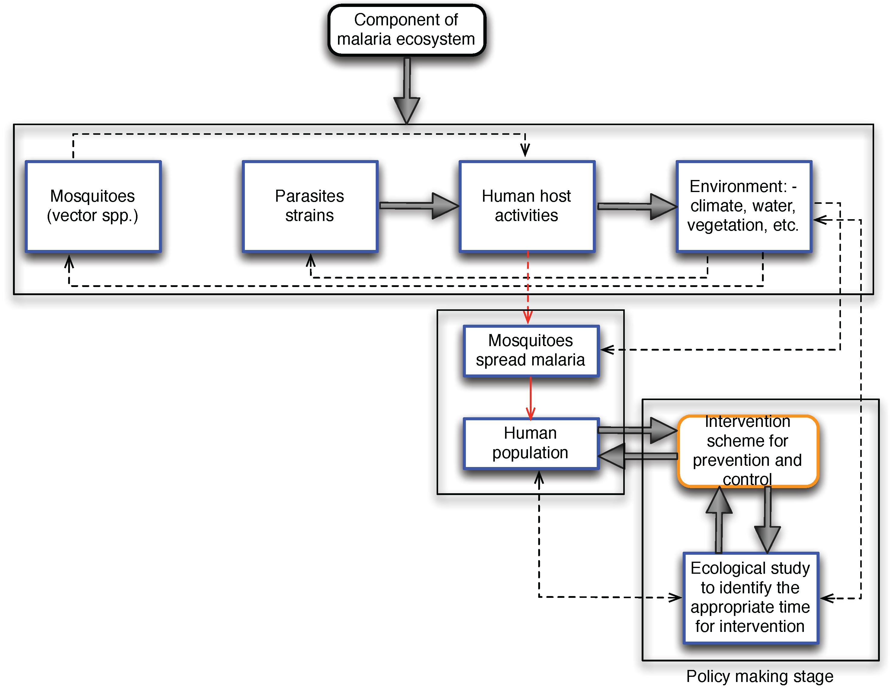
The malaria ecosystem comprises four main components: human host, mosquitoes vector, parasites and environmental condition (see Figure 1).
These components are very dynamic in nature due to the inherent characteristics of ecology and the anticipatory change to biodiversity because of global warming. The works by [15,16,17] reported that ecological changes would adversely affect human health in some ways that are both obvious and obscure. However, the growing evidence also suggests that due to the rise in temperature as a result of the anticipated global warming, some previously unexposed regions of malaria transmission would have a 50% chance of experiencing it due to the link between malaria incidence and ecological factors [18]. The relationship between environmental changes and human health cannot be overemphasized because of the inherent variability and complexity of human nature. In many circumstances, grasslands and forest are converted for agriculture to reduce communicable disease, including wetland drainage for the prevention and control of malaria [17]. These activities can either lead to unintended negative health effects or succeed in the designed purpose. Also, transforming forest to augment food production may, in the long run, lead to the creation of a suitable environment for disease-causing agents such as mosquitoes for malaria transmission [19].
2.1. Study Site and Population
Ejisu-Juaben Municipal has a population of 143,762 [20], lies within latitudes 115 N and 145 N also with longitudes 615 W and 700 W, occupies a land area of 582.5 km [21]. The vegetation of the municipal is a typical semi-deciduous forest (see Figure 2), with undulating topography and low altitude of about 240 m–300 m above sea level [21]. Also, the rainfall pattern of the area is bi-modal (i.e., two distinct seasons in a year), characterized by major and minor rainfall. The major rainfall begins from March to July with average annual rainfall between 1200 mm–1500 mm, while the minor rainfall begins in September and tapers off in November with annual average rainfall of 900 mm–1120 mm. Usually, December through February is hot, dry and dusty with mean annual temperature 25 C–32 C, and the relative humidity is moderately high during the rainy seasons [21]. Figure 2 presents the map of Ejisu-Juaben Municipal, which lies within the red-squared portion labelled Kumasi—the capital city of the Ashanti Region, in southern Ghana.
2.2. Data Collection and Source
A total of 85,627 confirmed diagnosed cases of malaria incidence for the period of five years from 2009 to 2013, were retrieved in [22]. The distributional pattern of malaria cases reported in the study area shows an indication of high malaria incidence. We sought data on climate factors in the designated weather station of the study area location [20]; unfortunately, very few data are available and also a lot are missing. This is perhaps due to laxity of the weather station staff for not properly keeping up-to-date data. Since the data available is not sufficient for the analysis, we overcome this challenge by using satellite-based meteorological data obtained via [23]. We used the boundary metrics dimensions of [22] at latitude 6.7989 N to 6.6823 S and longitude −1.5656 W to −1.4186 E and demarcate the location of the study area on the satellite globe map. Within the demarcated area, we identify a weather station. We then generate the data of the climate variables of our interest. Moreover, the Ghana malaria incidence data is sufficient for the application of PLS-PM due to its suitability for handling small sample data, non-normality, multi-dimensions and multicollinearity [24,25]. However, the sample set is not sufficient to obtain high precision accuracy when applying machine learning algorithms. A small dataset might also cause the overfitting of data. For that reason, we coupled malaria incidence data used in [26] with [22] and proceed with the analysis.
2.3. Factor Analysis
Exploratory factor analysis (EFA) is one of the techniques for factor analysis (FA). It is primarily used in statistics to describe variance among observed correlated variables in terms of potentially a smaller number of unobserved variables, usually referred to as factors [27]. In this work, EFA was employed to search for confounding ecological factors that are latent [8,27] from the set of observed meteorological variables.
We demonstrate the FA technique using simple mathematical sketches; the observed variables can be expressed as linear combinations of the potential factors plus the residual terms. Consider the following observed variables of size M, and assume they are linearly related to a small number of unobservable (latent variables) factors , with such that:
where are the residual terms, assuming that , and . While the unobservable factors are independent from each other and and . These two assumptions stand as the robust pre-conditions for the application of structural equation modelling (SEM). The loading scores can be obtained from covariance and variance of any two observed variables using the following formula presented in Equation (2)
where the summation sign in Equation (2) denotes communality of the variables, the variance of which is explained by the common factors .
2.4. Structural Equation Modelling
The SEM is a very popular technique that has multidisciplinary applications which combine together both the measurement and structural models [28,29,30]. In Figure 3a, we present a complex hypothetical SEM showing the causal relationship between malaria incidence and latent ecological factors together with their observed variables. We used ellipse shapes to represent latent factors, while the observed variables are represented by rectangular shapes.
2.5. Estimation of PLS-PM
The technique called PLS-PM or PLS-SEM was developed by [31] and chosen due to its characteristics in terms of small sample size, non-normality, multi-dimensions, and multicollinearity [23,24]. We have identified three hidden factors using EFA, and subsequently applied SEM for construction of the model (see Figure 3b). The PLS-PM is basically divided into three components: estimation of LVs, estimation of inner and outer models and estimation of the structural relations. The PLS algorithm is essentially represented as a sequence of regression in terms of weight vectors [32] and estimates the values of LVs (factor scores) iteratively until convergence is achieved. The fundamental PLS algorithm, as suggested by [30] (see Appendix A.1, Appendix A.2 and Appendix A.3 for detailed procedural descriptions). The PLS-PM is a component-based estimation technique that uses an iteration algorithm, separately analyzes the blocks of the measurement model and estimates the path coefficients in the structural model [33]. We used a package called semPLS in R for the estimation of PLS-SEM parameters including the analysis presented in Section 2.6.
For estimating parameters of SEM, we invoked the PLS technique, and further used 10,000 samples for the bootstrapping analysis instead of the default number of samples set to 500 selections [33]. Also, the PLS-PM latent variable scores were expressed as a linear combination of their observed variables and treated as an error-free substitute for the observed variables [33].
2.5.1. Measurement Model
The model, presented in Figure 3b, shows how observed Measurement Variables (MVs) are related to their Latent Variables (LVs). Hence without any loss of generality, for a good representation of the inner model, the following assumptions must hold:
- Matrix of MVs are scaled to have zero mean and unit variance.
- Each block of MVs is already transformed to be positively correlated for all LVs .
The measurement model is broadly classified as either reflective (Mode A) or formative (Mode B) [26], and this depends on the relation between LVs and MVs formation.
2.5.2. Mode A
In this form, each block of MVs reflects its LV and can be represented in multivariate regression form as:
where the can be estimated using the least squares method.
2.5.3. Mode B
Also, in this form, the LV is considered to be formed by its MVs represented by a multiple regression as:
using the same method of least squares, the estimate for can be obtained.
2.6. Presentation of Results
In the application of PLS-SEM, three weighting schemes such as centroid weighting, factorial weighting and path weighting are conceptually used for model specifications and estimations. The conceptual SEM presented in Figure 3a shows the hypothetical causal relationship between latent (hidden) variables and observed meteorological (manifest) variables to the occurrence of malaria incidence. For the identification of confounding hidden variables, we performed factor analysis using exploratory factor analysis (EFA) [34]. From the results, three hidden factors were identified: Factor I (related to the minimum temperature and relative humidity), Factor II (related to the maximum temperature and solar radiation) and Factor III (related to precipitation and wind speed). The identified factors accounted for 64% of the total variance, and at = 5% level of significance, = 13.91, df = 8, Pvalue = 0.0841. This result provides sufficient evidence to explain malaria incidence in the study area.
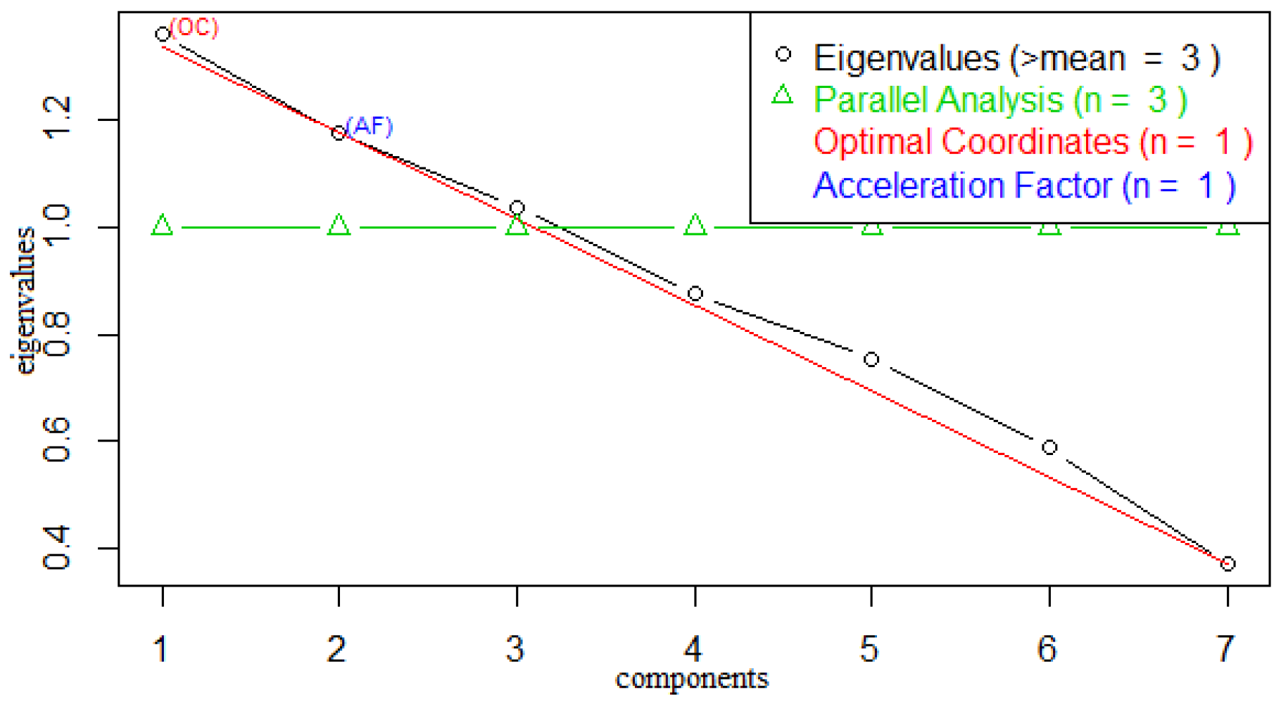
We also explored the Guttman–Kaiser Criterion [35] and Cattell scree plots [36], to determine the number of factors to extract, the result of which reconfirmed the existence of three hidden ecological factors to the incidence of malaria. In the Guttman–Kaiser Criterion, we have the eigenvalues 2.71, 1.53, 1.02, 0.82, 0.57, 0.29, 0.05 computed using the correlation matrix (see Table 1); however, the rule for extraction is based on the factors whose eigenvalues are greater than unity. We then discard those factors that have eigenvalues less than unity, and are left with three eigenvalues indicating the number of factors to be considered. Similarly, the Cattell scree plot presented in (Figure 4) facilitates decisions regarding the number of factors to retain.
By analysing Table 1, we obtained the scree plot shown in Figure 4 which represents the relative proportion of variance accounted for by the components. In the scree plot, the eigenvalues of the first three components greater than unity can be seen from the parallel indicator, while the subsequent components below unity also line up beneath the parallel indicator. However, it is important to evaluate the variance accounted for by a few of the eigenvalues regarded as sufficient so that we can focus on them and discard the remaining insufficient factors as noise.
In Table 2, we present Pearson’s cross-correlation between meteorological variables and occurrence of malaria incidence at various lag effects from 0 to 3 months. The Lag 0, Lag 1 and Lag 2 (e.g., 0 month, 1 month and 2 month) presented in Table 2 which indicates the lagged correlation effects between climate variables and the incidence of malaria in the study area. We observed that at lag effects of 1 month, the minimum temperature, maximum temperature and relative humidity have positive association with malaria incidence as indicated by 0.321, 0.215 and 0.254 respectively. While the precipitation is negatively correlated with malaria incidence at lag effects of 1 month as indicated by −0.292. This explained that the climate drivers at lag of 1 month would be quite enough for the mosquitoes to reproduce and also complete their incubation periods (EIP) to becomes fully active in transmitting malaria infection. We found that the preceding result is consistent with other relevant studies on the influence of meteorological variables on the malaria incidence [37]. The 1 month time lag in the study area is sufficient to capture the pattern of malaria transmission for various strains of plasmodium parasites with definite lengths of EIP. This period usually takes about 10–15 days [38] and temporally varies over location, parasite species and climatic resolution. At Lag 0 and Lag 2, the minimum temperature, precipitation and relative humidity have negative lag effects at 0 month and 2 month except the maximum temperature which has effects of 0.284 and 0.092. These results revealed some clear indications that the malaria transmission in the study area at Lag 0 and Lag 2 suffered a negative effect, which might be attributed to the bi-annual rainfall pattern, low relative humidity—say less than 50%—and inability of mosquitoes completing the EIP cycle. In general, the result showed that maximum temperature, minimum temperature, and relative humidity were related to the malaria incidence at lagged effects of 1 month (i.e., a month in advance) except precipitation which has a negative association in the study area.
Some important summary statistics are presented in Table 2, which describe the distributional pattern of the climate indicators of malaria incidence and variance inflated factor (VIF). In factor analysis, multicollinearity can be used as a diagnostics check prior to application of regression analysis, whereby variables with high-factor loadings are typically multicollinear. We compute VIF of the climate variables to measure the degrees of multicollinearity and identify those factors that are independent of the magnitude of their VIF. In Table 2, the minimum temperature and relative humidity have VIF of 8.7919 and 9.0065 that gives a high degree of multicollinearity. The results revealed a high independent predictor of malaria incidence in the study area, and the degree to which they are independent gives evidence to accurately determine the major factors. However, the values of kurtosis (see Table 2) indicate a high peak of the climate variables with positive values across all the indicators except the wind speed which indicates a flat distribution. Positive values, generally listed in Table 2, indicate that the peakedness of distribution of the climate variables particularly influences the malaria incidence. Also, the standard error estimates provide information on the statistical accuracy of the climate variables; the larger the standard error, the wider the confidence interval of the statistic and vice-versa.
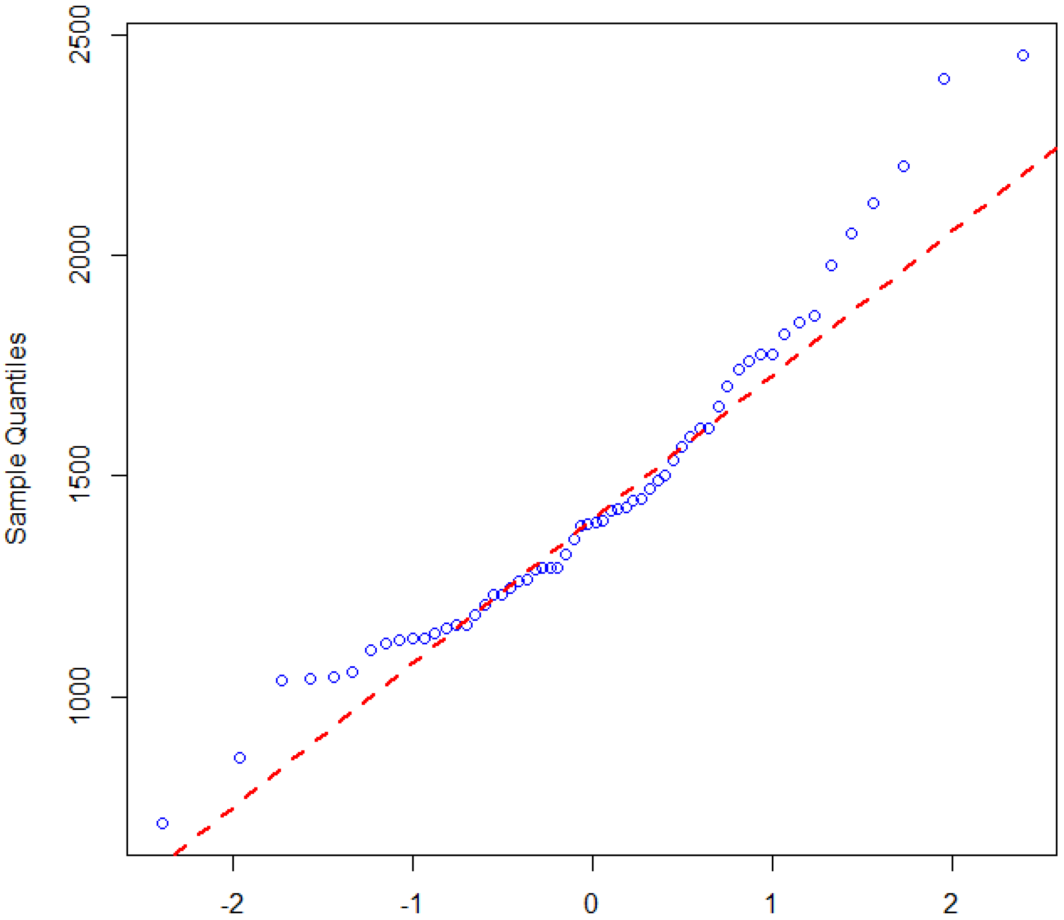
Non-normality of the dataset is one necessity for adopting PLS-SEM, and it is very robust when used on extremely non-normal data [39]. We examined the degree to which the data on malaria incidence are non-normal using the Shapiro–Wilk tests by invoking R software (3.4.1, University of Aukland, New Zealand). The results show that the null hypothesis (Ho) is rejected, indicating that the malaria incidence dataset is non-normal as suggested by the following indices W = 0.9486, p-value = 0.0134 and = 0.05, respectively. This method is particularly chosen and useful in smaller samples sizes, less than 2000 [40], and the null hypothesis is that the data are from a normal distribution. Similarly, we used a graphical approach called quantile–quantile (Q–Q) plot [41] and tested for normality of the dataset in similar fashion. The approach creates a plot from the ranked samples of the dataset against a similar number of ranked theoretical samples from a normal distribution. The plot shown in Figure 5, clearly indicates that the data points for malaria incidence are deviating from the straight line. Hence, the malaria incidence dataset is therefore not normally distributed using the Q–Q plot.
In Table 3, we show the results of the factor score estimates for path coefficients of SEM estimated using PLS path modelling, and three different structural model weighting schemes were analysed. We observed that Centroid (A) converges faster after 12 iterations, while factorial (B) and path weighting (C) converge after 15 iterations. The procedure of selecting the best weighting scheme is determined by the maximum number of iterations that will be used for calculating the PLS results and this algorithm did not stop until the maximum number of iterations is reached due to the stop criterion. From Table 3, we can observe that the B and C weighting schemes converge at the same maximum number of iterations in estimating the parameters of SEM. The weighting scheme provides the highest R value for endogenous latent variables in the PLS path model specifications and estimations. This result shows that the C weighting scheme is better than A and B, as suggested by [42] in terms of robustness and also when the path model includes higher-order constructs.
Table 4 presents the results of bootstrapping sampling for outer loadings of the observed variables and path coefficient of the latent variables estimated using PLS-PM. The results also show that all outer loadings and path coefficients are significant at = 5%, except for the solar radiation with Factor II and wind speed with Factor III that contains zero-point in the bootstrap confidence interval. Furthermore, the interaction effects of the Factors between I and II, II and III were also investigated and the results revealed that none of the Factor combinations is significant in the incidence of malaria in the study area. This result provides sufficient evidence that high malaria incidence in the study area was attributed to the occurrence of minimum temperature and relative humidity which are identified as Factor I.
The decision to select the most influential hidden ecological factor to the incidence of malaria is based on the communality and Dillon–Goldstein’s indices. Furthermore, Table 5 summarizes the results, indicating some indices for selecting the hidden ecological factors to the high incidence of malaria in the study area. Among the three factors identified by EFA, we find that Factor I, indicated by minimum temperature and relative humidity, influences malaria transmission with communality index (0.94) and Dillon–Goldstein’s (0.97). This result is also consistent with the finding in [37], where a positive association exists between temperature and occurrence of dengue. Factor II and Factor III appear to have less influence on the malaria incidence.
3. Intelligent Malaria Outbreak Warning System
In the previous section, we identified the hidden ecological factors of malaria using partial least squares path modelling. In this section, we discuss, in detail, the implementation of the malaria outbreak system, based on the identified hidden ecological factors. The deployment comprises of three stages: data processing, generating the predictive model using machine learning and deployment of a mobile application.
3.1. Data Preprocessing
It was a tradition, prior to the application of machine learning algorithms, that datasets need to be pre-processed to enable a faster and more accurate learning process. The heuristic approach involves the discretization techniques most often used in data mining. This involves transforming continuous-valued datasets to discrete datasets by creating a set of contiguous intervals [43]. In this paper, we are making use of a dataset on climate variables as the input while the output variable is malaria incidence data. Our concern is the development of a predictive model using supervised machine learning algorithms that will predict the likelihood of malaria incidence. The output variable appeared to have high-magnitude in-terms of reported number of malaria cases; hence using it directly may cause over-fitting to the predictive model. Therefore, it is pertinent to transform the dataset using some techniques for discretization to enable us to build efficient models.
We have therefore discretized the output variable to form a target variable using the k-means clustering algorithm [44]. This methodology is chosen over equal width (EW) and equal frequency (EF) because it is less sensitive to outliers and also the number of clusters (partitions) can be optimized by analysis rather than pre-determination. In general, the choice of discretization method and choice of k can be guided by the objectives of the discretization task. By invoking R software, we can determine the optimum number of clusters to enable us to partition the output variable.
From the analysis, the optimum number of clusters obtained is k = 4 and the algorithm converges after nine iterations with 89.9% variation. Also, we observed that for k = 5, the number of iterations exceeded the maximum number of tolerable iterations supposed to achieve convergence and in this case it diverges even though the percentage of variation is still good at 93%. For k = 2 and 3, the algorithm converges after three and four iterations with 66.4% and 82% variation, respectively. This gives sufficient evidence to choose the optimum number of clusters as k = 4. Similarly, we have also tried the “NbClust” package in R software for determining the optimal number of clusters. Using the values of k ranging from two to five allows the algorithm to select the optimum number of clusters to be used in order to partition the output variable. The algorithm run and selected k = 4 as the optimum number of clusters to partition the output variables. Hence, both methodologies give the same number of optimum clusters to consider and subsequently prove to be consistent. We then partitioned the output variable into four classes according to the results of k-means algorithm and re-labeled them as: low, medium, high and very high incidence status of malaria. We present, in Table 6, the summary analysis of k-means algorithm clustering.
3.2. Machine Learning
The next stage is to identify a pattern/model from the data processed in Section 3.1 that will be used to make an accurate prediction of malaria incidence. Evolved from traditional pattern recognition approaches, machine learning methods explore the algorithms that can learn from the data and overcome prediction tasks by building a mathematical model with a data sample input. A learning algorithm will mark each given Malaria epidemic data sample as one category, then after being trained using the training dataset, it will build a model to predict which category a forthcoming data sample falls into.
We have applied several machine learning algorithms, including Support Vector Machine (SVM), K-Nearest Neighbours (KNN), Naive Bayes and Decision Trees, to find the best predicting algorithm from the scikit framework [45] in Python.
To evaluate the prediction of machine learning algorithms on the training set, we have used the 10-fold cross-validation technique by selecting a training set and test sets that are mutually independent. Table 7 shows the prediction results in comparison to seven different Machine Learning methods.
- Linear Regression (LiR) method gives overall good prediction results, but it seems that the method failed to produce any medium predictions.
- Logistic Regression (LoR) method predicts the probability of occurrence of an event by fitting the dataset, as a set of independent variables, into a logic function. In other words, for a correlated data set, LoR may not be able to find the intrinsic-relationships between events.
- Decision Tree (DT) works very well for both categorical and continuous dependent variables; however, this dataset cannot be separated as distinct groups since the edges of the samples are fuzzy. Therefore, DT gave a bad prediction after all.
- Support Vector Machine (SVM) is one of the most efficient supervised machine learning algorithms, which is mainly used for solving classification and regression problems. The best part of this algorithm is that training and testing data can be plotted as a point in a n-dimensional plane, with a feature being the value of a particular coordinate. Without optimisation of the parameters, SVM gave a 80.56% predicting result. After parameter optimisation, especially on the penalty parameter and gamma coefficient adjustment, SVM (o) gave a 99.0% predicting result.
- Naive Bayes (NB) is a well-known classification method, which is based on Bayes’ Theorem with an oversimplified assumption of independence between classifiers. Moreover, NB is a conditional probability model, which means that the method needs to be assigned a series of certain events. For this data set, NB did not produce a good prediction overall.
- K-Nearest Neighbours (KNN) method is able to deal with both classification and regression problems. In comparison to KNN5 (where k = 5) and KNN10 (where k = 10), KNN1 (where k = 1) failed to make a good prediction. It means that the data may need to do more pre-process and/or noise removal in a theory; however, most of data from the real world are incomplete; that is why KNN5 and KNN10 make a better prediction.
- K-Means (K-M) is a type of un-supervised method for clustering. In this case, three clusters have been set at the beginning; however, a convergence did not perfectly land; therefore, it cannot give a good overall prediction.
The results, presented in Table 7, show that the best performing algorithm is SVM. We therefore integrate the SVM model into our system.
3.3. Mobile Application
We have developed a mobile application, Malaria Outbreak Warning System, with a built-in SVM model, published at Google Play. The tool can be accessed via [46].
The application is based on the theoretical experiences and practical experiments of the SVM algorithm and model, which has been tested for developing systematic and effective strategies to predict the outbreak of a Malaria epidemic. Meanwhile, the parameters of the model kernel have been optimised and set into this application.
The application consists of three processes: pre-processing the weather forecasting data, processing the data by applying them into the model and implementing the model’s interface, and post-processing the prediction data by presenting results on the app’s UI front layer. It is a well-suited implementation for location detection.
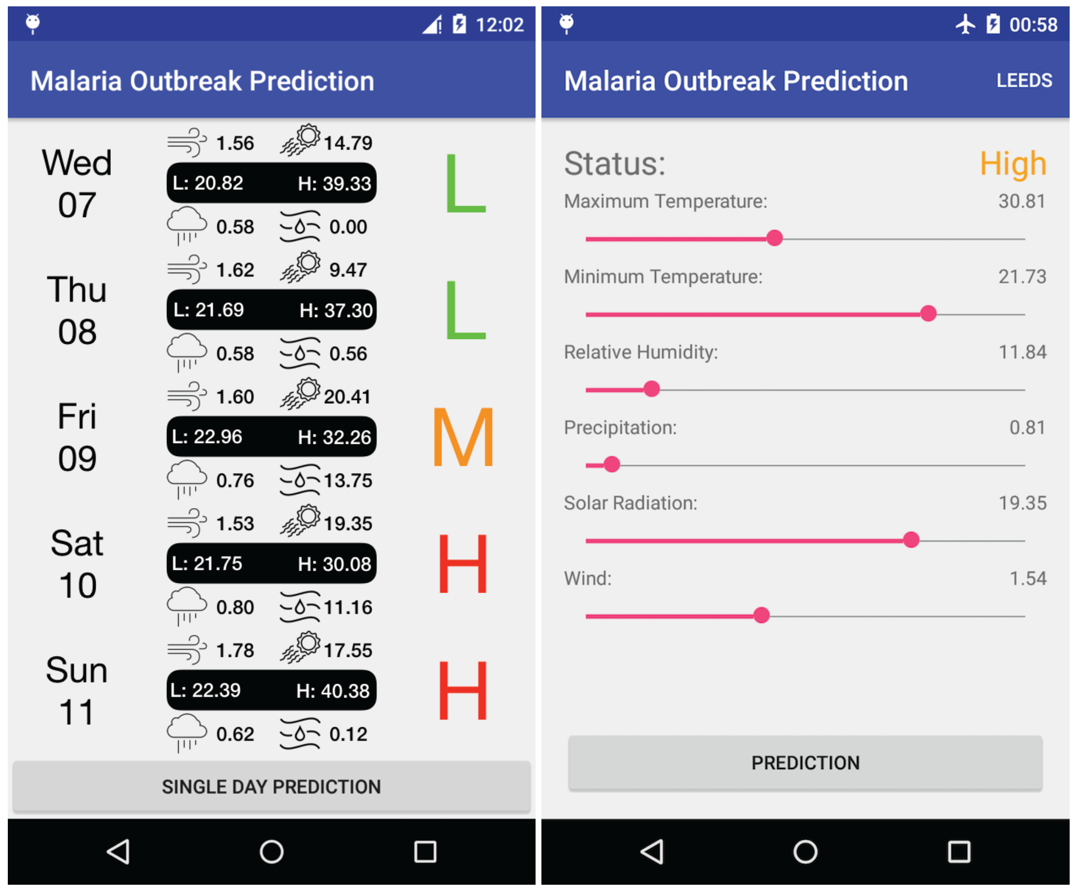
Figure 6 shows a screen shot of the tool. The application not only supports the automatic gathering of weather forecasting data, but also supports manual data input. The application reads climatic information, i.e., temperature, relative humidity, wind speed, solar radiation and precipitation, from the weather and geographical APIs. When the units of the weather and atmosphere are different from the data set used to construct the predictor, we carry out the required normalisation or feature scaling or similar pre-processing. The tool then predicts the Malaria outbreak a couple of days in advance based on available forecast information acquired from the APIs. The user can slide the screen to see the available outbreak predictions for the current and future days. The additional button on the bottom of the screen is to let the user manually enter a set of weather measurements to make a prediction for customised parameters.
The trained SVM model has been implemented in Java by taking advantage of the LIBSVM (2.88, University of California, Berkeley, CA, USA) [47]. LIBSVM is an integrated software for SVM, regression and distribution estimation. The mobile application has been developed for Android using Android Studio. The weather forecasting data is powered by OpenWeatherMap API (3.0, Riga, Latvia) [48], which is an online service provider for weather data. OpenWeatherMap provides API for searching forecasting data for up to 5 days by coordinates; and the responses served as JavaScript Object Notation (JSON), Extensible Markup Language (XML) and HyperText Markup Language (HTML) endpoints. All of the data provided is under CC BY-SA 4.0 license.
3.4. Discussion
The current prototype of the intelligent malaria outbreak warning system relies on a batch machine learning process. That is, the learning algorithm is trained and tested offline using the available dataset, and the prediction model is embedded within the tool. Hence, the prediction process relies on the prediction model trained offline at once.
A more effective approach is to make the learning process online. That is, whenever new data is available, the data is automatically updated, and the learning process is run again to encapsulate the new data. This will not only allow an automatic and dynamic learning process, but also increase the accuracy of the prediction by adapting to new patterns in the data.
The online learning approach requires a mechanistic data collection mechanism, which is very challenging to perform as hospitals and health service providers do not make the relevant data available online. Even acquiring permission to have access to the available data is a long and bureaucratic process. On the other hand, as discussed in Section 2.2, most available data cannot be directly used in this system as they are incomplete and/or not processed.
To alleviate these issues and to support the online learning process, the Malaria outbreak warning application can be extended to collect online data from its users. Namely, the users, e.g., hospitals, healthcare providers, individuals etc., report a Malaria case to the system. Using the geographical location of the incident, the application will acquire all the necessary information for the ecological factors. In this way, new data will be collected at run time, and the learning process will be instantiated each time new data is available. We are currently working on the development of this approach.
4. Conclusions
In this study, we have deployed an intelligent malaria outbreak early warning system, predicting malaria outbreaks based on climatic factors using machine learning algorithms. The system will help hospitals, healthcare providers, and health organizations take precautions in time and utilize their resources in case of emergency. To our best knowledge, the system developed in this paper is the first publicly available application.
We have also provided an ecosystem overview for malaria modelling and proposed a new framework for the study of a malaria transmission ecosystem to prevent and control its effects. We have assessed and identified hidden factors that lead to a high malaria outbreak. Our data analysis results have shown that the minimum temperature and relative humidity, which are related to Factor I, have a positive association with the incidence of malaria in the study area. The other observed variables such as maximum temperature, solar radiation, precipitation and wind speed, which are related to hidden Factor II and Factor III, appear to have mildly influenced malaria incidence.
The primary results obtained in this study have demonstrated the power of the proposed predicative analytics-based malaria outbreak warning system. The further development of the system will incorporate automatic data gathering from a variety of sources. We are currently working on further development of our system and methodology to support automatic data collection at run time, and the online learning process. This will not only allow an automatic and dynamic learning process, but also increase the accuracy of the prediction by adapting to new patterns in the data.
Acknowledgments
The authors would like to thank National Centre for Environmental Prediction (NCEP), for their support in providing this work with relevant meteorological data. The author B.M. would like to thank Tertiary Education Trust Fund (tetFund), Nigeria for sponsoring his Ph.D. programme at the University of Bradford, UK. Y.L and S.K. acknowledge Innovate UK KTP010551 grant.
Author Contributions
Savas Konur, Nereida Polovina, Yang Lan, A. Taufiq Asyhari and Yonghong Peng designed the experiments; Babagana Modu performed the experiments; Babagana Modu analysed the data; Babagana Modu, Savas Konur, Nereida Polovina, Yang Lan, A. Taufiq Asyhari and Yonghong Peng contributed reagents/materials/analysis tools; Babagana Modu wrote the paper.
Conflicts of Interest
The authors declare no conflict of interest.
Abbreviations
The following abbreviations are used in this manuscript:
| SEM | Structural Equation Modelling |
| EFA | Exploratory Factor Analysis |
| PLS-PM | Partial Least Squares Path Modelling |
| LVs | Latent Variables |
| MVs | Measurement Variables |
| FA | Factor Analysis |
| API | Application Programming Interface |
| SVM | Support Vector Machine |
| LiR | Linear Regression |
| LoR | Logistic Regression |
| DT | Decision Tree |
| NB | Naive Bayes |
| KNN | K-Nearest Neighbours |
| K-M | K-Means |
| CFSR | Climate Forecast System Reanalysis |
| NCEP | National Centre for Environmental Prediction |
| JSON | JavaScript Object Notation |
| XML | Extensible Markup Language |
| HTML | HyperText Markup Language |
Appendix A
Appendix A.1. Estimation of Parameters
- Step 1
- Initialization: Suppose are the respective MVs, and are scaled such that and . We are interested in expressing each LV as a linear combination of MVs, represented in compact form:Hence, the LVs are initialized as: .
- Step 2
- Inner approximationWithin the inner model domain, the estimation of the path parameter of each LV can be mathematically represented as the weighted sum of its neighbouring LVs.The approximate estimation of the inner model path parameter takes: .
- Step 3
- Outer approximationThe outer approximation is computed based on the weight of the LV loads from the inner approximation. This comes in two forms, Mode A and Mode B. For Mode A, a multivariate regression coefficient with the block of MVs as the response and the LV as the regressor:Mode B is a multiple regression coefficient with the block of MVs as the response and its block of MVs as the regressor:
- Step 4
- Outer weight vectorLet be a set of indices for MVs related to LV ; then, , , is a column vector of length . We can write down the matrix of outer weights, W as:The outer weight vectors, , in an outer weights matrix W, which we are using now to estimate the factor scores by means of the MVs, areresulting in the outer estimation: .
- Step 5
- Iteration
Appendix A.2. Weighting Scheme
The weighting schemes are used to estimate the inner weight in (A2) of the PLS algorithm. Generally, there are three weighting schemes, centroid [49], and later [42] introduced the factorial and path weighting schemes.
Appendix A.2.1. Centroid (A)
The centroid weighting scheme takes the form:
where denotes the matrix of inner weights.
Appendix A.2.2. Factorial (B)
The factorial weighting scheme also takes the form:
Appendix A.2.3. Path Weighting (C)
In this weighting scheme, the predecessor and successor of a LV play a different role in the relation. The relation between one specific LV and its successor is determined by their correlation; for the predecessors it is determined by a multiple regression
where is the predecessor set of the LV . Denoting as the successor set of the LV ; the elements of the inner weight matrix are denoted as
Appendix A.3. Discriminant Validity Check
In the structural equation model, the factor scores are estimated by the PLS algorithm, while the path coefficients are also estimated using ordinary least squares (OLS). Now, for each LV , , the path coefficient is the regression coefficient in its predecessor set defined as:
Using (A11), we can compute the element , of the estimated matrix of path coefficients .
Appendix A.3.1. Path Coefficients
Appendix A.3.2. Total Effects
We can calculate the matrix of the total effects as the sum of the 1 to step transition matrices:
Note that expands to , e.g., contains all the indirect effects mediated by only one LV.
Appendix A.3.3. Outer Loadings
The cross and outer loadings are estimated as:
References
- World Health Organization. Malaria Rapid Diagnostic Test Performance: Results of WHO Product Testing of Malaria RDTs: Round 6; World Health Organization: Geneva, Switzerland, 2015. [Google Scholar]
- Haque, U.; Hashizume, M.; Glass, G.E.; Dewan, A.M.; Overgaard, H.J.; Yamamoto, T. The role of climate variability in the spread of malaria in Bangladeshi highlands. PLoS ONE 2010, 5, e14341. [Google Scholar] [CrossRef] [PubMed]
- Bonan, G.B.; Shugart, H.H. Environmental factors and ecological processes in boreal forests. Annu. Rev. Ecol. Syst. 1989, 20, 1–28. [Google Scholar] [CrossRef]
- Kumar, V.; Mangal, A.; Panesar, S.; Yadav, G.; Talwar, R.; Raut, D.; Singh, S. Forecasting malaria cases using climatic factors in Delhi, India: A time series analysis. Malar. Res. Treat. 2014. [Google Scholar] [CrossRef] [PubMed]
- Ngarakana-Gwasira, E.T.; Bhunu, C.P.; Masocha, M.; Mashonjowa, E. Assessing the Role of Climate Change in Malaria Transmission in Africa. Malar. Res. Treat. 2016. [Google Scholar] [CrossRef] [PubMed]
- Nath, D.C.; Mwchahary, D.D. Association between Climatic Variables and Malaria Incidence: A Study in Kokrajhar District of Assam, India: Climatic Variables and Malaria Incidence in Kokrajhar District. Glob. J. Health Sci. 2013, 5, 90. [Google Scholar]
- Modu, B.; Asyhari, A.T.; Peng, Y. Data Analytics of climatic factor influence on the impact of malaria incidence. In Proceedings of the 2016 IEEE Symposium Series on Computational Intelligence (SSCI), Athens, Greece, 6–9 December 2016; pp. 1–8. [Google Scholar]
- Tenenhaus, M.; Vinzi, V.E.; Chatelin, Y.M.; Lauro, C. PLS path modeling. Comput. Stat. Data Anal. 2005, 48, 159–205. [Google Scholar] [CrossRef]
- Sriram, T.; Rao, V.; Narayana, S.; Dowluru, K. Intelligent Parkinson disease prediction using machine learning algorithms. Int. J. Eng. Innov. Technol. 2013, 3, 212–215. [Google Scholar]
- Ganesan, N.; Venkatesh, K.; Rama, M.A. Application of Neural Networks in diagnosing cancer disease using demographic data. Int. J. Comput. Appl. 2010, 1, 76–85. [Google Scholar] [CrossRef]
- Aditya, M.; Prince, K.; Himanshu, A.; Pankaj, K. Early heart disease prediction using data mining techniques. Comput. Sci. Inf. Technol. 2014, 53–59. [Google Scholar] [CrossRef]
- Wang, L. (Ed.) Support Vector Machines: Theory and Applications; Springer: Berlin, Germany, 2005; Volume 177. [Google Scholar]
- Sharma, V.; Kumar, A.; Panat, L.; Karajkhede, G.; Lele, A. Malaria outbreak prediction model using machine learning. Int. J. Adv. Res. Comput. Eng. Technol. 2015, 4, 4415–4419. [Google Scholar]
- Parham, P.E.; Michael, E. Modelling the effects of weather and climate change on malaria transmission. Environ. Health Perspect. 2010, 118, 620. [Google Scholar] [CrossRef] [PubMed]
- Myers, S.S.; Patz, J.A. Emerging threats to human health from global environmental change. Annu. Rev. Environ. Resour. 2009, 34, 223–252. [Google Scholar] [CrossRef]
- Myers, S.S.; Gaffikin, L.; Golden, C.D.; Ostfeld, R.S.; Redford, K.H.; Ricketts, T.H.; Osofsky, S.A. Human health impacts of ecosystem alteration. Proc. Natl. Acad. Sci. USA 2013, 110, 18753–18760. [Google Scholar] [CrossRef] [PubMed]
- Bayles, B.R.; Brauman, K.A.; Adkins, J.N.; Allan, B.F.; Ellis, A.M.; Goldberg, T.L.; Ricketts, T.H. Ecosystem Services Connect Environmental Change to Human Health Outcomes. EcoHealth 2016, 13, 443–449. [Google Scholar] [CrossRef] [PubMed]
- The Potsdam Institute for Climate Impact Research and Climate Analytics. Turn-Down the Heat—Why a 4 Degree Warmer World Must Be Avoided; International Bank for Reconstruction and Development and World Bank: Washington, DC, USA, 2012. [Google Scholar]
- De Castro, M.C.; Monte-Mór, R.L.; Sawyer, D.O.; Singer, B.H. Malaria risk on the Amazon frontier. Proc. Natl. Acad. Sci. USA 2006, 103, 2452–2457. [Google Scholar] [CrossRef] [PubMed]
- Nyarko, P. Population and Housing Census, District Analytical Report, Ejisu-Juaben Municipal. Available online: https://www.citypopulation.de/php/ghana-admin.php?adm2id=0117. (accessed on 12 January 2017).
- Addai, G.; Anyatewon Kwesi, D. 2010 Population and Housing Census: District Analytical Report, 1st ed.; Ghana Statistical Service: Accra, Ghana, 2014.
- Takyi Appiah, S.; Otoo, H.; Nabubie, I.B. Times Series Analysis Of Malaria Cases In Ejisu-Juaben Municipality. Int. J. Sci. Technol. Res. 2015, 4, 220–226. [Google Scholar]
- Global Weather Data for SWAT. Available online: http://globalweather.tamu.edu (accessed on 24 June 2017).
- Nitzl, C.; Chin, W.W. The case of partial least squares (PLS) path modeling in managerial accounting research. J. Manag. Control 2017, 28, 137–156. [Google Scholar] [CrossRef]
- Bagozzi, R.P.; Yi, Y. Specification, evaluation, and interpretation of structural equation models. J. Acad. Mark. Sci. 2012, 40, 8–34. [Google Scholar] [CrossRef]
- Dan, E.D.; Jude, O.; Idochi, O. Modelling and forecasting malaria mortality rate using SARIMA models (a case study of Aboh Mbaise general hospital, Imo State Nigeria). Sci. J. Appl. Math. Stat. 2014, 2, 31–41. [Google Scholar] [CrossRef]
- Ruscio, J.; Roche, B. Determining the number of factors to retain in an exploratory factor analysis using comparison data of known factorial structure. Psychol. Assess. 2012, 24, 282. [Google Scholar] [CrossRef] [PubMed]
- Kline, R.B. Principles and Practice of Structural Equation Modelling; Guilford Publications: New York, NY, USA, 2015. [Google Scholar]
- Kelloway, E.K.; Santor, D.A. Using LISREL for Structural Equation Modelling: A Researcher’s Guide. Can. Psychol. 1999, 40, 381. [Google Scholar]
- Monecke, A.; Leisch, F. SemPLS: Structural Equation Modeling Using Partial Least Squares. J. Stat. Softw. 2012, 48, 1–32. [Google Scholar] [CrossRef]
- Wold, H. Soft Modeling: The Basic Design and Some Extensions. In Systems under Indirect Observation: Causality– Structure– Prediction; Part 2; Jöreskog, K.G., Wold, H., Eds.; North-Holland Publishing Company: Amsterdam, The Netherlands, 1982; pp. 1–54. [Google Scholar]
- Dijkstra, T.K. Latent variables and indices: Herman Wold’s basic design and partial least squares. In Handbook of Partial Least Squares; Springer: Berlin, Germany, 2010; pp. 23–46. [Google Scholar]
- Byrne, B.M. Structural Equation Modelling with LISREL, PRELIS, and SIMPLIS: Basic Concepts, Applications, and Programming; Psychology Press: Hove, UK, 2013. [Google Scholar]
- Li, X.X.; Wang, L.X.; Zhang, J.; Liu, Y.X.; Zhang, H.; Jiang, S.W.; Zhou, X.N. Exploration of ecological factors related to the spatial heterogeneity of tuberculosis prevalence in PR China. Glob. Health Action 2014, 7. [Google Scholar] [CrossRef] [Green Version]
- Yeomans, K.A.; Golder, P.A. The Guttman-Kaiser criterion as a predictor of the number of common factors. Statistician 1982, 31, 221–229. [Google Scholar] [CrossRef]
- Ledesma, R.D.; Valero-Mora, P.; Macbeth, G. The scree test and the number of factors: A dynamic graphics approach. Span. J. Psychol. 2015, 18. [Google Scholar] [CrossRef] [PubMed]
- Xu, L.; Stige, L.C.; Chan, K.S.; Zhou, J.; Yang, J.; Sang, S.; Lu, L. Climate variation drives dengue dynamics. Proc. Natl. Acad. Sci. USA 2016, 114, 113–118. [Google Scholar] [CrossRef] [PubMed]
- Srinivasulu, N.; Gujju Gandhi, B.; Naik, R.; Daravath, S. Influence of Climate Change on Malaria Incidence in Mahaboobnagar District of Andhra Pradesh, India. Available online: https://www.ijcmas.com/Archives/vol-2-5/N.%20Srinivasulu,%20et%20al.pdf (accessed on 24 June 2017).
- Hair, J.F.; Sarstedt, M.; Pieper, T.M.; Ringle, C.M. The use of partial least squares structural equation modelling in strategic management research: A review of past practices and recommendations for future applications. Long Range Plan. 2012, 45, 320–340. [Google Scholar] [CrossRef]
- Jarque, C.M.; Bera, A.K. A test for normality of observations and regression residuals. Int. Stat. Rev./Rev. Int. Stat. 1987, 55, 163–172. [Google Scholar] [CrossRef]
- Wilk, M.B.; Gnanadesikan, R. Probability plotting methods for the analysis for the analysis of data. Biometrika 1968, 55, 1–17. [Google Scholar] [CrossRef] [PubMed]
- Lohmöller, J.B. Latent Variable Path Analysis with Partial Least Squares; Physica-Verlag: Heidelberg, Germany, 1989. [Google Scholar]
- Lustgarten, J.L.; Gopalakrishnan, V.; Grover, H.; Visweswaran, S. Improving classification performance with discretization on biomedical datasets. In Proceedings of the AMIA Annual Symposium, Hilton Washington and Tower, Washington, DC, USA, 8 November 2008. [Google Scholar]
- Maslove, D.M.; Podchiyska, T.; Lowe, H.J. Discretization of continuous features in clinical datasets. J. Am. Med. Inf. Assoc. 2013, 20, 544–553. [Google Scholar] [CrossRef] [PubMed]
- Scikit-Learn. Available online: http://www.scikit-learn.org (accessed on 24 June 2017).
- MLSVM for Research. Available online: https://play.google.com/store/apps/details?id=project.lanydr.mlsvm&hl=en (accessed on 24 June 2017).
- LIBSVM-A Library for Support Vector Machines. Available online: www.csie.ntu.edu.tw/~cjlin/libsvm/ (accessed on 24 June 2017).
- Weather API. Available online: http://openweathermap.org/api) (accessed on 24 June 2017).
- Gang, S. Soft modeling: Intermediate between traditional model building and data analysis. In Mathematical Statistics; Polish Scientific Publishers: Warsaw, Poland, 1980; Volume 6, pp. 333–346. [Google Scholar]
Figure 1.
Conceptual framework of the malaria ecosystem describing the dynamic stages of malaria transmission from humans and mosquitoes under the influence of environmental factors. The boxes colored blue indicates the dynamics development of malaria parasite and its interaction between human host with mosquito vector and ecology. While the box colored red is the main scheme for malaria prevention and control indicating the intervention measure taken to mitigate the burden imposed on the human population.

Figure 2.
The picture on the left shows the map of Ghana and the portion of Kumasi city, where the study area within which Ejisu-Juaben lies. The picture on the right illustrates the climate vegetational belt characterized by a typical semi-deciduous forest.
Figure 2.
The picture on the left shows the map of Ghana and the portion of Kumasi city, where the study area within which Ejisu-Juaben lies. The picture on the right illustrates the climate vegetational belt characterized by a typical semi-deciduous forest.
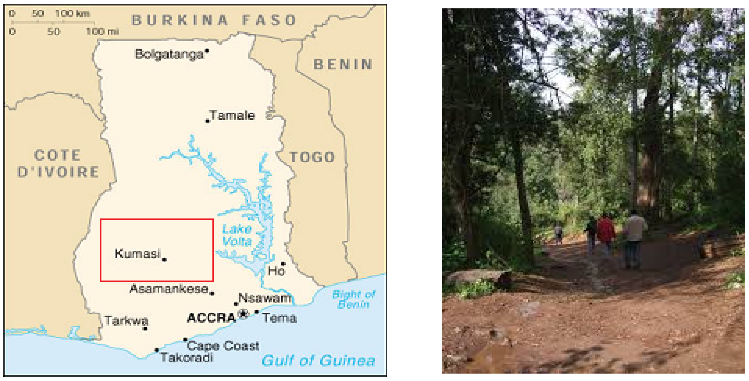
Figure 3.
Structural equation model showing the relationship between malaria incidence and climate factors, the black colored rectangle indicating measurement variables while red colored ellipse is latent variables. (a) Showing the hypothetical causal relationship between malaria incidence and the climate factors. (b) Presenting the reduced causal relationship between malaria incidence and the climate factors after applying factor analysis to identify hidden factors and their dependent measurement variables.
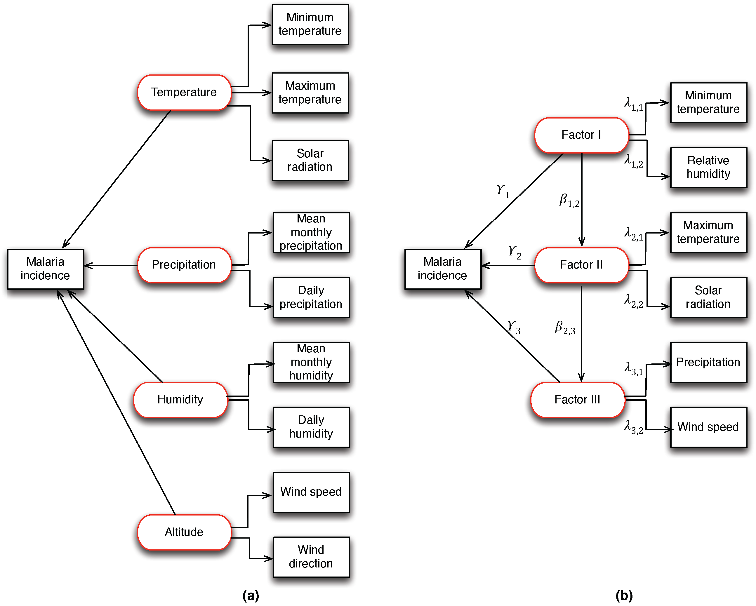
Figure 4.
The Cattell scree plot presents the eigenvalues of the components and threshold for identifying the number of hidden ecological factors to be considered using the information in Table 1.
Figure 4.
The Cattell scree plot presents the eigenvalues of the components and threshold for identifying the number of hidden ecological factors to be considered using the information in Table 1.

Figure 5.
Graphical representation of quantile–quantile (Q–Q) plot normality tests.

Figure 6.
A screen shot of the mobile application.


Table 1.
Correlation matrix of climate drivers and malaria incidence.
| Mal. Incid. | Max. Temp. | Min. Temp. | Precip. | Rel. Humid | Solar Rad. | Wind Speed | |
|---|---|---|---|---|---|---|---|
| Mal. Incid. | 1.00 | - | - | - | - | - | - |
| Max. Temp. | 0.28 | 1.00 | - | - | - | - | - |
| Min. Temp. | 0.68 | 0.04 | 1.00 | - | - | - | - |
| Precip. | −0.21 | −0.36 | 0.22 | 1.00 | - | - | - |
| Rel. Humid. | 0.51 | −0.24 | 0.90 | 0.38 | 1.00 | - | - |
| Solar Rad. | 0.19 | 0.54 | −0.33 | −0.10 | −0.44 | 1.00 | - |
| Wind Speed | −0.16 | 0.07 | 0.45 | 0.17 | 0.39 | 0.01 | 1.00 |
Note: (1) Malaria incidence, (2) Maximum temperature, (3) Minimum temperature, (4) Precipitation,
(5) Relative humidity, (6) Solar radiation and (7) Wind speed.
Table 2.
Cross-correlation between meteorological variables and malaria incidence; VIF:variance inflated factor.
Table 2.
Cross-correlation between meteorological variables and malaria incidence; VIF:variance inflated factor.
| Variables | Lag 0 | Lag 1 | Lag 2 | VIF | Kurtosis | Standard Error |
|---|---|---|---|---|---|---|
| Maximum temperature | 0.284 | 0.321 | 0.092 | 2.4096 | 5.48 | 0.38 |
| Minimum temperature | −0.122 | 0.215 | −0.237 | 8.7919 | 2.07 | 0.33 |
| Precipitation | −0.214 | −0.292 | −0.155 | 1.4194 | 20.73 | 0.27 |
| Relative humidity | −0.134 | 0.254 | −0.198 | 9.0065 | 1.42 | 0.02 |
| Solar radiation | - | - | - | 1.9000 | 6.73 | 0.50 |
| Wind speed | - | - | - | 1.3452 | −0.58 | 0.04 |
a negative association at lag 1. b positive association at lag 1.
Table 3.
Factor scores for path coefficients in the PLS-PM using three weighting schemes.
| Measurement/Structural Model | Parameter | Estimate | Centroid (A) | Factorial (B) | Path Weighting (C) |
|---|---|---|---|---|---|
| Minimum temperature ⟵ FactorI | 0.9479 | 0.9479 | 0.9495 | 0.9495 | |
| Relative humidity ⟵ FactorI | 0.9910 | 0.9910 | 0.9903 | 0.9903 | |
| Maximum temperature ⟵ FactorII | 0.8816 | 0.8816 | 0.8675 | 0.8675 | |
| Solar radiation ⟵ FactorII | 0.8735 | 0.8735 | 0.8873 | 0.8873 | |
| Precipitation ⟵ FactorIII | 0.9849 | 0.9849 | 0.9852 | 0.9852 | |
| Wind speed ⟵ FactorIII | 0.0017 | 0.0017 | 0.0031 | 0.0031 | |
| FactorI ⟶ FactorII | −0.3248 | −0.3248 | −0.3302 | −0.3302 | |
| FactorII ⟶ FactorIII | −0.2774 | −0.2774 | −0.2690 | −0.2690 | |
| FactorI ⟶ Malaria incidence | 0.9700 | - | - | - | |
| FactorII ⟶ Malaria incidence | 0.7700 | - | - | - | |
| FactorIII ⟶ Malaria incidence | 0.4900 | - | - | - | |
| Maximum number of iterations | - | - | 12 | 15 | 15 |
Table 4.
Bootstrapping test of the outer loadings and path coefficients in the PLS-PM with a 95% confidence interval.
Table 4.
Bootstrapping test of the outer loadings and path coefficients in the PLS-PM with a 95% confidence interval.
| Measurement/Structural Model | Parameter | Estimate | Bias | Standard Error | Lower | Upper |
|---|---|---|---|---|---|---|
| Minimum ⟵ FactorI | 0.9479 | −0.0057 | 0.0467 | 0.8240 | 0.9890 | |
| Relative humidity ⟵ FactorI | 0.9910 | −0.0055 | 0.0347 | 0.9823 | 1.0000 | |
| Maximum temperature ⟵ FactorII | 0.8816 | −0.0329 | 0.1289 | 0.4769 | 0.9810 | |
| Solar radiation ⟵ FactorII | 0.8735 | −0.0343 | 0.1748 | −0.0705 | 0.9550 | |
| Precipitation ⟵ FactorIII | 0.9849 | −0.1748 | 0.4044 | 0.7666 | 1.0000 | |
| Wind speed ⟵ FactorIII | 0.0017 | 0.1356 | 0.4059 | −0.6593 | 0.7300 | |
| FactorI ⟶ FactorII | −0.3248 | −0.0333 | 0.1692 | −0.4974 | 0.4260 | |
| FactorII ⟶ FactorIII | −0.2774 | −0.0264 | 0.2191 | −0.4963 | 0.3810 |
Table 5.
Indices for selecting the ecological hidden factor of high malaria incidence in the study area.
Table 5.
Indices for selecting the ecological hidden factor of high malaria incidence in the study area.
| Factor | Reflective Variables | Communality | Dillon–Goldstein’s |
|---|---|---|---|
| I | 2 | 0.94 (94%) | 0.97 (97%) |
| II | 2 | 0.77 (77%) | 0.87 (87%) |
| III | 2 | 0.49 (49%) | 0.49 (49%) |
c the most significant hidden factor.
Table 6.
Summary of data discretization using the k-means algorithm. SSB: The sum of squares of errors between the clusters; SST: The total sum of squares of the entire clusters.
Table 6.
Summary of data discretization using the k-means algorithm. SSB: The sum of squares of errors between the clusters; SST: The total sum of squares of the entire clusters.
| Number of Clusters (k) | 2 | 3 | 4 | 5 |
|---|---|---|---|---|
| iteration | 3 | 4 | 9 | 6 |
| convergence | yes | yes | yes | no |
| 66.4% | 82% | 89.9% | 93% |
Table 7.
Comparison of the accuracy of model checking algorithms. LiR: Linear Regression; LoR: Logistic Regression; DT: Decision Tree; SVM: Support Vector Machine; SVM (o): Optimized Support Vector Machine; NB: Naive Bayes; KNN: K-Nearest Neighbours; K-M: K-Means.
Table 7.
Comparison of the accuracy of model checking algorithms. LiR: Linear Regression; LoR: Logistic Regression; DT: Decision Tree; SVM: Support Vector Machine; SVM (o): Optimized Support Vector Machine; NB: Naive Bayes; KNN: K-Nearest Neighbours; K-M: K-Means.
| Algorithm | LiR | LoR | DT | SVM | SVM (o) | NB | KNN1 | KNN5 | KNN10 | K-M (3) |
|---|---|---|---|---|---|---|---|---|---|---|
| Accuracy | 83.8% | 75.0% | 63.8% | 80.6% | 99.0% | 63.9% | 58.3% | 80.6% | 80.6% | 47.2% |
© 2017 by the authors. Licensee MDPI, Basel, Switzerland. This article is an open access article distributed under the terms and conditions of the Creative Commons Attribution (CC BY) license (http://creativecommons.org/licenses/by/4.0/).
Share and Cite
MDPI and ACS Style
Modu, B.; Polovina, N.; Lan, Y.; Konur, S.; Asyhari, A.T.; Peng, Y. Towards a Predictive Analytics-Based Intelligent Malaria Outbreak Warning System. Appl. Sci. 2017, 7, 836. https://doi.org/10.3390/app7080836
AMA Style
Modu B, Polovina N, Lan Y, Konur S, Asyhari AT, Peng Y. Towards a Predictive Analytics-Based Intelligent Malaria Outbreak Warning System. Applied Sciences. 2017; 7(8):836. https://doi.org/10.3390/app7080836
Chicago/Turabian StyleModu, Babagana, Nereida Polovina, Yang Lan, Savas Konur, A. Taufiq Asyhari, and Yonghong Peng. 2017. "Towards a Predictive Analytics-Based Intelligent Malaria Outbreak Warning System" Applied Sciences 7, no. 8: 836. https://doi.org/10.3390/app7080836
Note that from the first issue of 2016, this journal uses article numbers instead of page numbers. See further details here.