Bisector-Based Tracking of In Plane Subpixel Translations and Rotations


1
Institute of Physics Applied to the Sciences and Technologies, Universidad de Alicante, Carretera San Vicente del Raspeig, s/n, San Vicente del Raspeig, 03690 Alicante, Spain
2
Department of Optics, Pharmacology and Anatomy, Universidad de Alicante, Carretera San Vicente del Raspeig, s/n, San Vicente del Raspeig, 03690 Alicante, Spain
3
Department of Civil Engineering, Universidad de Alicante, Carretera San Vicente del Raspeig, s/n, San Vicente del Raspeig, 03690 Alicante, Spain
*
Author to whom correspondence should be addressed.
Appl. Sci. 2017, 7(8), 835; https://doi.org/10.3390/app7080835
Submission received: 17 July 2017
/
Revised: 9 August 2017
/
Accepted: 11 August 2017
/
Published: 14 August 2017
(This article belongs to the Section Optics and Lasers)
Abstract
:We present a method for distance measuring planar displacements and rotations with image processing methods. The method is based on tracking the intersection of two non-parallel straight segments extracted from a scene. This kind of target can be easily identified in civil structures or in industrial elements or machines. Therefore, our method is suitable for measuring the displacement in some parts of structures and therefore for determining their stress state. We have evaluated the accuracy of our proposal through a computational simulation and validated the method through two lab experiments. We obtained a theoretical mean subpixel accuracy of 0.03 px for the position and 0.02 degrees for the orientation, whereas the practical accuracies were 0.1 px and 0.04 degrees, respectively. One presented lab application deals with the tracking of an object attached to a rotation stage motor in order to characterize the dynamic of the stage, and another application is addressed to the noncontact assessment of the bending and torsional process of a steel beam subjected to load. The method is simple, easy to implement, and widely applicable.
1. Introduction
In the last years, computer vision systems have been demonstrated to be an efficient tool to accurately track movements and vibrations, mainly in those applications where contact measurement is inadequate. The majority of applications rely on displacement tracking, which is also a key parameter in structures in order to evaluate their security under loading.
Local displacements can be described through cross-correlation, which allows an investigator to obtain the relative position between two identical images [1]. This correlation can be applied on specific targets as well as on distinct object parts. The advantages of cross-correlation are widely known. Unfortunately, it also has some disadvantages. Among them, because of its linear formulation, it has a strong dependence on the scene luminance. Also, it has a limited spatial accuracy, and, additionally, it only stands for displacement tracking but not for object rotations. The first issue has been addressed through normalized cross-correlation [2], and the second through smart interpolation of the scene or the correlation peak itself [3]. Solving the third problem is not so easy, and it is necessary to usually make use of a mathematical transformation of both the scene and the target prior to the cross-correlation operation [4,5,6].
Measuring rotations and torsions is of great importance for completely describing the movements and forces acting on a structure [7]. Traditionally, this movement is described indirectly through local displacements by using contact methods. The measured shifts may be then decomposed in order to separate real displacement from torsions and rotations, thus introducing calculation noise and a level of uncertainty into the movement determination. Additionally, contact measurements are adequate in controlled environments and small parts, but the cost–benefit ratio in real structures is really high, thus impeding its use in this case.
In our opinion, it would be of great interest to design a noninvasive method capable of tracking object displacements and rotations simultaneously, even in big elements located far away from the measuring point. In the published literature, one can find different methods used to image rotation measurement, such as phase-encoded grayscale image correlation [8], which is used to measure rotation at a constant interval of 3° using holographic storage; double phase-encoded correlation [9], which provides results with absolute errors of 0.22 degrees and around 0.12 px in the determination of the rotation and the displacement, respectively; log polar correlation [5,6], which is able to detect translation, rotation, shear, and scale changes with an angle resolution of 0.7 degrees for a 512 × 512 log-polar representation [10]; Hilbert wavelet transformation [11], which allows an investigator to obtain out-of-plane rotations at steps of 15 degrees; and holographic optical correlator methods [12], which are able to measure the rotation of the image as accurately as 0.05 degrees. However, in spite of the variety of approaches to the problem, we find that some of them [8,9] can be sensitive to certain kinds of noise that make them not suitable for some practical applications, and others [6,11] may require computationally intensive calculations or are of limited application because of low computing accuracy [12].
On the other hand, the position and orientation of an object can also be obtained by calculating some object features, like the centroid and second-order moments of the image’s intensity distribution [13]. However, these techniques can impose constraints on the target morphology or on scene illumination in order to facilitate the detection of these features. In certain cases, these constraints cannot be met due to the nature of the system or the limitations of the experiment, and, additionally, if the selected features are too restrictive, they might be inadequate for tracking complex motions.
In [14], the authors proposed a technique to track translations within the image plane xy of an object without using a specific target or template-matching techniques, but with the specific need of the object image having two nonparallel straight segments. They tracked displacements with an accuracy of hundredths of a pixel, or even of thousandths of a pixel in the case of tracking harmonic vibrations. The motion of the object is described by tracking the intersection of two straight lines obtained from the digitization of the two segments from the scene, which allows an investigator to locate that point with a subpixel resolution. Unfortunately, the object tracking is done through a single-point target, which does not provide information about changes of orientation.
In this paper, we propose a significant improvement of the technique presented in [14] and simultaneously obtain information about the object’s position and orientation in the image plane with subpixel accuracy. The method explained below exactly locates the object using a vector consisting of the coordinates (xc, xc) of the intersection of two nonparallel straight lines and the angle (β) with the horizontal axis of one of the bisectors of the angles between those lines.
The manuscript is structured as follows. In the next section, we describe the theoretical basis of the technique. The Method section is set for explaining the algorithm developed to compute these parameters. In order to check the performance of this technique, we propose a theoretical simulation and two lab experiments in the fourth section, in which we describe those experiments and discuss the obtained results. Finally, the main conclusions of this paper are outlined.
2. Conceptual Approach
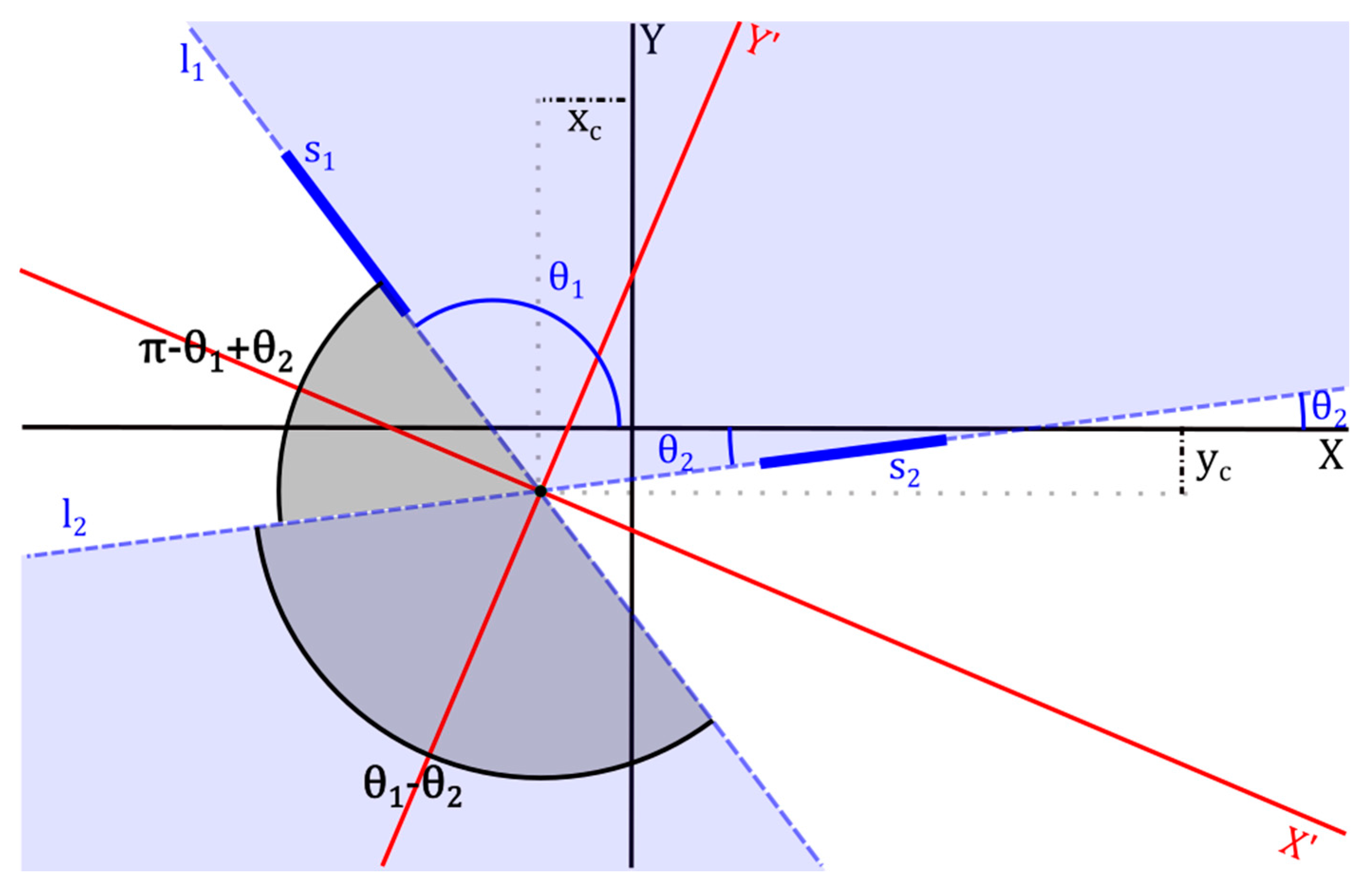
Let us consider a simple object in Figure 1 consisting of two nonparallel straight segments s1 and s2. The straight lines that best fit to these segments are li, with i = 1, 2, and they fulfil Equation (1):
where bi are the y-intercepts of each line, and θi are the angles with respect the abscises axis. The straight lines intersect in a point (xc, xc) that can be used to locate the position of the object [14].
As we said above, by only tracking the lines’ intersection, we are not able to distinguish orientation changes, and thus the object’s movement will only be partially described. Therefore, we need an extra parameter that provides information on the orientation of the assembly formed by the two segments. To this end, the trivial solution is selecting the angle between them, e.g., (θ1 − θ2) in Figure 1. Obtaining all of the describing parameters, i.e., the crossing point and the angle between segments, implies computing the four unknown parameters in (1). Although valid, this procedure has two main drawbacks. The first is that it considers the two segments as independent from one another, so it does not inform about the shape invariance of the target as a whole. The second drawback is that a combination between two independent adjustments may increase the errors, thus making an unreliable method for tracking small movements.
Here, we propose an alternative method that overcomes those drawbacks. If the object is rigid and its shape does not change, the Equation in (1) can be transformed and linked to reduce the number of unknowns, and then the accuracy of the tracking algorithm would be increased. Following with Figure 1, the straight lines define two pairs of opposite angles in the plane. These angles are divided into two equal parts by the lines called angle bisectors. The bisectors can be used as axes of a new Cartesian system due to the fact that they perpendicularly intersect. Hence, they form a coordinates system centred at the intersection point (xc, xc) that moves with the object. Therefore, our proposal is not solving the Equation in (1) but to find the new coordinates system formed by the bisectors and track its movement. In that way, we reduce the unknown to three: the coordinates of the intersection point (xc, xc), or equivalently, how much the original coordinates system must be translated to match the intersection with the origin, and the angle (β), which means how much the original coordinates system must be rotated to match the axes with the bisectors. Therefore, the aim now is to compute vector (xc, xc, β) that locates (X’, Y’) in position and orientation.
A particular feature of the Cartesian system formed by the bisectors is that the axes act as reflecting axes of symmetry, i.e., the specular reflection of one of the lines relative to one of the axes coincides with the other line. This can be observed in Figure 2, where we have represented the rotated and re-centred version of the scheme depicted in Figure 1. There, , the reflection of s1 with respect to X’, matches with the line l2. Therefore, both straight lines l1 and l2 referred to (X′, Y′) are equivalent if we change the sign of one of the coordinates to one of them (2). Thus, this feature can be used as a condition to link Equation (1) and to obtain (xc, xc, β).
3. Methods
We have developed an algorithm that allows an investigator to compute the location vector (xc, yc, β) from a video sequence of a moving object using a function minimization algorithm. Next, we describe the algorithm step by step.
The first step consists of image processing to obtain edge binary images. The particular method followed in this stage may vary depending on the video sequence, although the result must be an edge binary image. After this, it is necessary to select by hand two masks that contain the two digitized nonparallel segments, s1 and s2. Inside each mask, the coordinates of the activated pixels define both segments in the initial Cartesian coordinates reference system, with the axes aligned with the rows and columns of the support matrix. The objective is to find (xc, yc, β) that transforms to , which describes the coordinates in one Cartesian system with the axes aligned with the bisectors between the two segments. Such a geometrical transformation changes the set of coordinates following:
where i = 1, 2 stands for the number of the segment and j = 1, …, Ni, being Ni the number of pixels that form each segment. It is just a composition of a geometrical translation and rotation, i.e., , where and are the rotation and translation matrices.
On the other hand, let us remember that in the Cartesian system formed by the bisectors, the data set that comprises the coordinates from one segment (s2 in the above example) and those from the reflection with respect to one axis of the other one (e.g., ) will lie on the same straight line. According to Figure 2, the Equation of the straight line that contains one segment, and the reflected version of the other with respect to one axis of the reference system (X’, Y’), can be expressed as:
We estimated the slope of Equation (4) from the result of separately fitting the coordinates of the segments to straight lines by solving the linear least-squares problem, described by:
Notice that, from Equation (5), we could have estimated the value of the location vector (xc, yc, β), provided that . In that case, as we claimed above, we would not take into account that the shape of the object does not change, and the result would be affected by the noise of two different fittings.
Alternatively, we geometrically transform the coordinates of the segments using different location vectors (xd, yd, φ), i.e., , until the mean squared error (MSE) between the transformed data and the straight line obtained from (4) is minimized.
where with k = 1, …, N1 + N2.
At this point, we would like to underline that there is no preference in the choosing of the segment that is reflected or in the choosing of the bisector with respect to that segment is reflected. In fact, the choice is irrelevant when we track a moving object in a video sequence, provided that we do not change the choice during the process. Selecting any option only implies that we obtain the orientation of the bisector at the angle β or at the complementary one. Both cases provide the same information, so from here onward and for simplicity, we only consider the angle β.
We use the Nelder–Mead simplex algorithm [15] in order to minimize (6) and obtain the optimum parameters (xc, yc, β). Basically, the algorithm repeatedly modifies the parameters of the transformation from an initial guess until it meets a stopping criterion. In our case, we made a blind search with no initial guess, i.e., (xd, yd, φ) = (0, 0, 0), and established a termination tolerance on the parameters of 10−8 and a maximum number of function evaluations allowed of 108.
An issue we must not forget is that the object is supposed to be in movement, so the defined masks should follow that movement in order to avoid a case where the segments fall out of them in any frame. What is done in order to not lose the object and to accelerate the calculation is to recalculate the coordinates of the masks every third frame. They are successively transformed according to the relative movement of the two previous frames. This way, we assume that the location variation frame to frame is similar during three frames of the sequence. In the case of a sudden steep change of movement, the segments would fall out of the masks, and the tracking would fail. This may be solved by increasing the frame rate of the camera in order to avoid a change from frame to frame that is sudden and steep. The algorithm finally provides (xc, yc, β)t, being t = 1, …, T, so relative translations and rotations between previous frames are:
4. Results
We propose a theoretical simulation and two real experiments to evaluate the performance of the presented technique. All processing was implemented offline using Matlab through a script that followed the steps depicted in the flow chart of Figure 3. Matlab offers a function named fminsearch with the Nelder–Mead simplex algorithm, and a function named lscov [16] that was used to compute the least-square solution that minimized the sum of squared errors.
4.1. Numerical Simulation
We created a sequence of frames with a rhombus that rotated 2 degrees in steps of 0.01 degrees with reference to a point, and we applied the proposed minimization technique to track the object. We assumed that we were able to obtain an edge binary image in the image-processing stage, and we have only isolated two nonparallel segments from the border of the object at each frame of the sequence. In Figure 4, we show a processed frame of the sequence (see Visualization 1) where both segments, the theoretical and the computed intersection point, the rotation centre, the computed bisector, and the orientation angle are plotted.
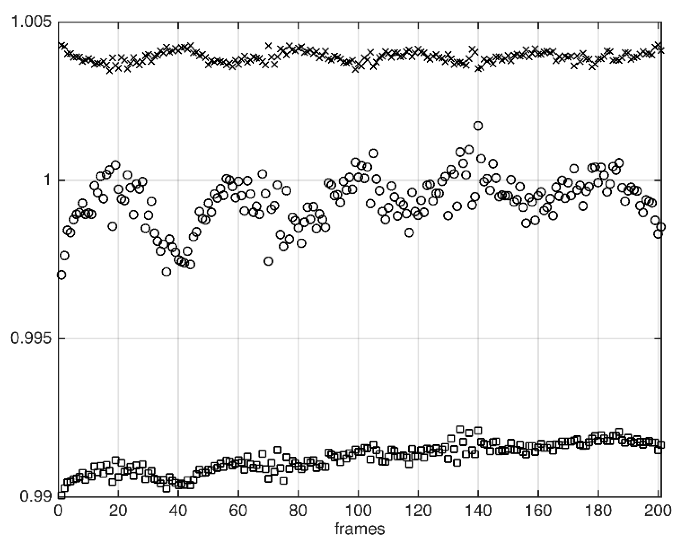
We have compared the computed intersections and orientations with the theoretical ones. They show a good correlation, with p-values <0.05 in all parameters and Pearson coefficients near one (0.99). This way, we have denoted the linear dependence existing between the computed and the theoretical location vector parameters. In Figure 5, we represent the quotient between them, computed at each frame of the sequence. Note that all are near one. The MSE resulting from the linear least-squared fittings (computed vs. theoretical ones) is 0.0010 for xc (crosses), 0.0028 for yc (squares), and 0.0005 for β (circles). With the standard deviation, we can set that the mean subpixel accuracy determining the position and the angle is to be 0.03 px and 0.02 degrees, respectively.
4.2. Experimental Results
4.2.1. Experimental Setups
● Rotation stage
We implemented an experiment consisting of an object attached to a motorized rotation stage (CR1-Z7), which was controlled by a motor controller (TDC001 DC) from Thorlabs. The stage provides continuous 360° travel, with a wobble and repeatability of less than 2 arcsec and 1 arcmin, respectively. We set a trajectory consisting of a rotation of 5 degrees, with a maximum angular acceleration αm = 0.5 deg/s2 and a maximum angular velocity ωm = 1 deg/s. The motion employed is described by a trapezoidal velocity profile: the stage is gradually ramped at an acceleration to a maximum velocity, and, as the destination is approached, the stage is decelerated so that the final position is slowly reached.
The object was a sheet with a calibrated grid and the printed logo of our University. The grid was used to facilitate the calculation of the pixel to millimetre ratio. The video sequence was recorded using a Nikon 5100 camera with a Nikkor 18–55 objective, a resolution of 25 fps and 1920 × 1080 px at a distance of 1 m from the object, which provided a spatial resolution equal to 4.4 px/mm. The whole scene was illuminated with a halogen projector.
● Mechanical torsion and bending in a beam
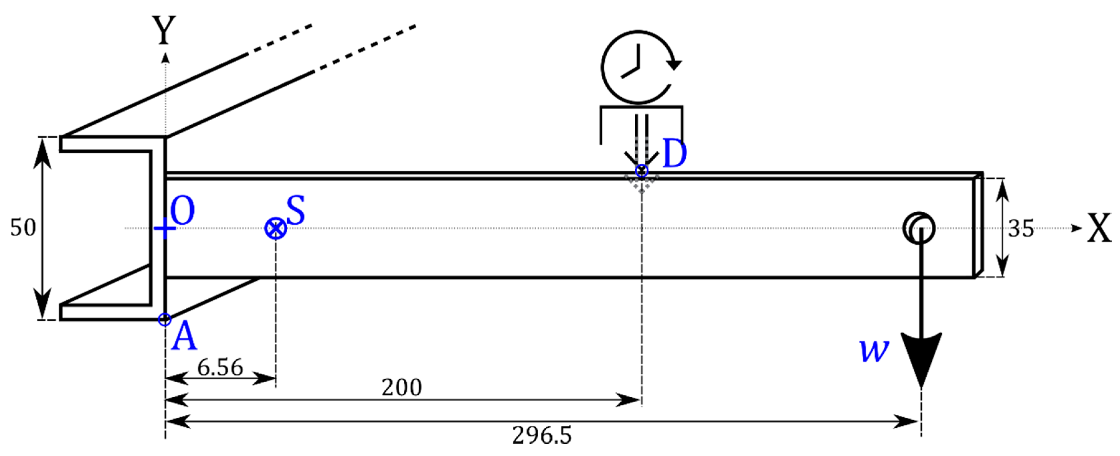
We have implemented another experiment aimed at measuring the torsion and bending of a cantilever steel beam with a 50 × 25 × 4 mm U cross-section and a length of 775 mm. In Figure 6, we show a scheme of the experimental setup. On the free end, a perpendicular plate is welded. In that plate, one can hang different weights from a hole located at 296.5 mm from point O. In our case, we used a weight w = 5 N. A displacement measurer was placed over the plate at xD = 200 mm from the point O in the X direction. It is used to measure the vertical displacement resulting from the combination of torsion and bending forces in the system. We used two Basler AC800-510uc video cameras with objectives Pentax TV lens of 25 mm recording at 300 frames per second (fps). One captured the distance measurer and the other one recorded the profile of the U-shape beam, specifically point A (0, −25) mm. The resolution obtained with this last camera was equal to 9.5 px/mm.
The bending and torsion of the experimental structure caused by a load of known weight w can be theoretically characterized using the moment-area theorems [17], by which we obtain the vertical displacements due to bending both in the U cross-section beam, , and in the perpendicular plate, , as well as the torsional angle in the cross-section beam for the point D, following:
where all distances are in millimeters, w in Newtons, and in radians. In our case, we got and . Due to the eccentric load, the section rotates around its shear center S that is located at xS = 6.56 mm. Due to the rotation of the U section, all points have an additional displacement, given by
where and are the distance of a point (x, y) to the shearing center, and γ indicates the direction from S to the point.
4.2.2. Video Processing and Object Tracking Calculation
The video sequences were processed offline following our own algorithm implemented in Matlab as we explained in the Method section.
● Rotation stage
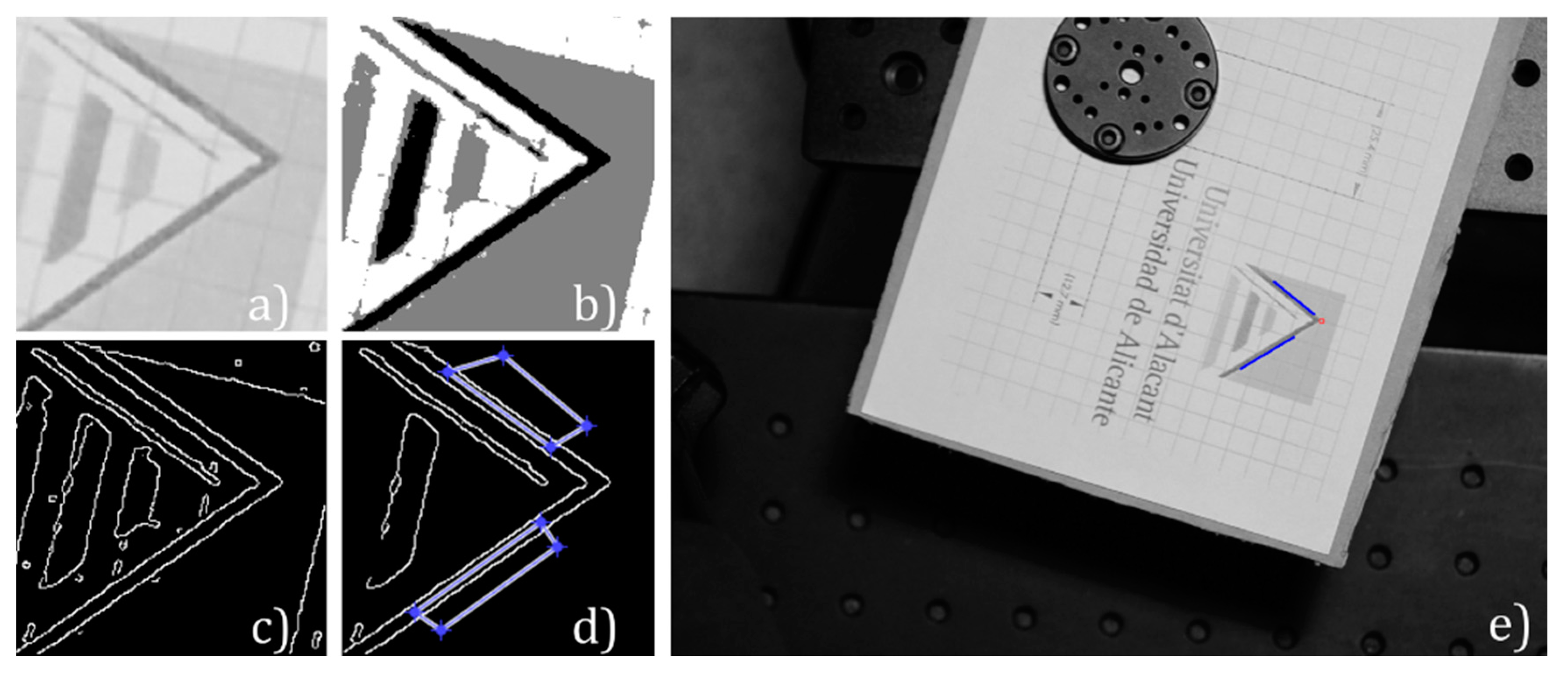
In Figure 7, we show images resulting from the main stages of the image processing algorithm used in the experiment of the rotation stage. The logo of our University was the object to be tracked, so, from each frame, we cropped a region where we expected to extract two nonparallel segments (Figure 7a). Then, we quantized the image using two quantization levels (Figure 7b) and extracted the edges (Figure 7c) using the Canny method [18]. Next, we applied a binary opening filter to remove objects smaller than 200 px, to avoid undesired interferences, and manually selected two regions of the processed image that contained the two nonparallel segments (s1 and s2) (Figure 7d). There, we got the coordinates of both segments. The two masks were automatically transformed frame to frame following the relative movement. We computed a location vector for each frame of the sequence. Figure 7e shows a frame of the sequence with the selected segments (blue) and the computed intersection (red square).
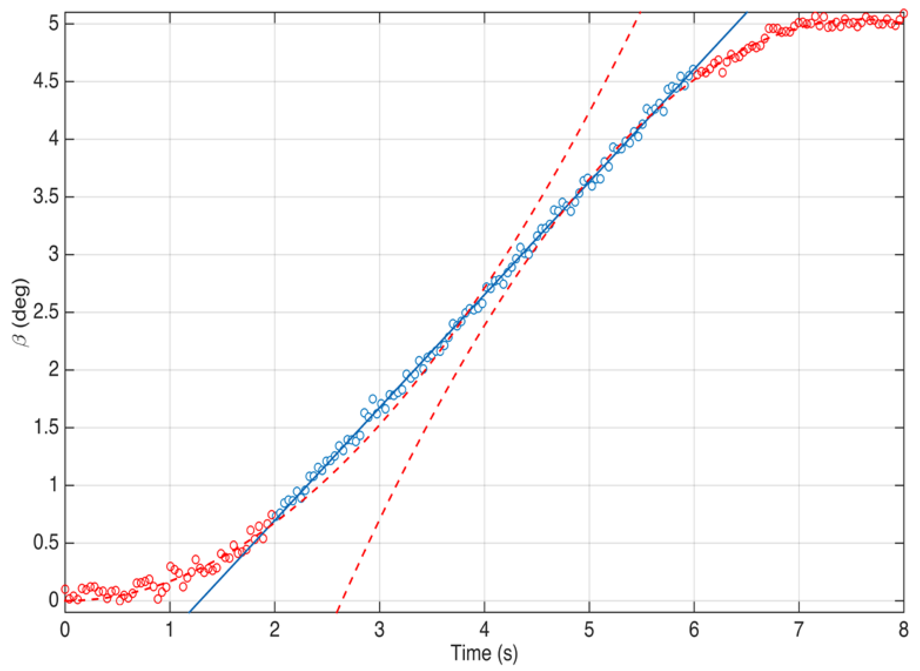
In Figure 8, we present the variation of the angle β of the computed location vector in time through the video. Since we were not able to compare the position with the theoretical value, we only evaluated the parameters of the rotation stage provided by the manufacturer. As it was said above, the trajectory was a rotation of 5 degrees, in accordance with the registered rotation. The start and the end of the curve correspond to the time intervals when the object is stopped. There, one can appreciate two extrema zones where the stage motor accelerates and decelerates, in concordance with the employed trapezoidal velocity profile. Between these zones, the stage theoretically reached a constant maximum angular velocity of 1 deg/s. We have approximately cropped these three zones in the curve and fitted them to uniformly accelerated and constant velocity movement Equations, and obtained significant correlations (p-value < 0.05). The first interval, which corresponds to the start of the engine until it reached constant velocity at around t = 2 s, was fitted assuming it was uniformly accelerated, i.e., . The initial acceleration resulted in deg/s2, with a Pearson coefficient R = 0.89. Next, approximately between t = 2 s and t = 6 s, the curve was fitted to the straight line with R = 0.99, thus assuming constant angular velocity movement. The slope resulted in 0.978 ± 0.004 deg/s, which deviates 2% from the maximum theoretical value, and s. At this instant, the angle in the uniformly accelerated phase would be degrees. Finally, we assumed that the rotation stage uniformly decelerated and fitted data from t = 6 s to the end to the curve . We constrained the angular velocity to be deg/s. We obtained deg/s2, s, and degrees, with R = 0.94.
Therefore, the proposed method allowed us to obtain angular acceleration and velocity with accuracies of hundredths of deg/s2 and thousandths of deg/s, respectively, besides tracking the position of the object (see Visualization 2). Under the assumption of being a motion consisting of a constant velocity phase between two uniformly accelerated ones, we have been able to determine the instants and angular positions limiting each motion phase.
● Mechanical torsion and bending in a beam
In this experiment, we obtained two video sequences: one from the camera recording the beam, and another one from the camera recording the contact distance measurer. On the one hand, the processing of the first video is again directed to obtain an edge binary image. The object to be tracked is the U-shape beam profile, so, from each frame, we cropped a region around the point A, where we expected to extract two intersecting segments. Then, we equalized the histogram of the image to enhance contrast and we binarized it. Straightaway, we extracted the edges using the Canny method [18], and applied an opening filter to remove small objects (those shorter than 200 px, in this case). In the final processed image, we manually selected two regions that contained the two nonparallel segments (s1 and s2), and got the coordinates of both segments. These regions were automatically transformed frame to frame following the relative movement. With those, we computed the location vector (xc, yc, β) for each frame of the sequence through the presented minimization method. In Figure 9, we show a frame of the sequence with the selected segments (blue), the computed intersection (red square), which coincided with the corner of the beam as expected, and the bisector (pink).
In Table 1, we present the results for the location vectors’ parameters computed separately solving (5), with those obtained by applying the proposed minimization method and the theoretical values obtained from (8) and (9). We can compare the errors and deviations obtained with both methods at point A with reference to the theoretical one. The torsional angle coincides with the variation of β. Its value obtained with the proposed method is quite similar to the theoretical one, with an absolute difference of 4 × 10⁻³ radians and a relative deviation of 18%, whereas the result obtained solving (5) differed around 0.02 radians with a relative deviation of 78%. The errors of the fittings in (5) probably accumulate, a fact that leads to a bad angle estimation, and therefore the method is dismissed.
By comparing the theory and the minimization method regarding the displacements, one can see that the deviation in the x-direction is similar to that of the angle. However, the deviation in the y-direction is quite higher. Note that the displacement magnitudes are low, so the signal-to-noise ratio is high and the measurements inaccurate, although the estimation is not bad. It is not worth comparing displacement values because those magnitudes are related to the torsional angle in Equation (9). Indeed, they are more sensitive to errors in the theoretical calculations. Note that the structure is not ideal (welding, holes, not squarely welded pieces, irregularities in the shape pieces, inhomegeneities in the material, …).
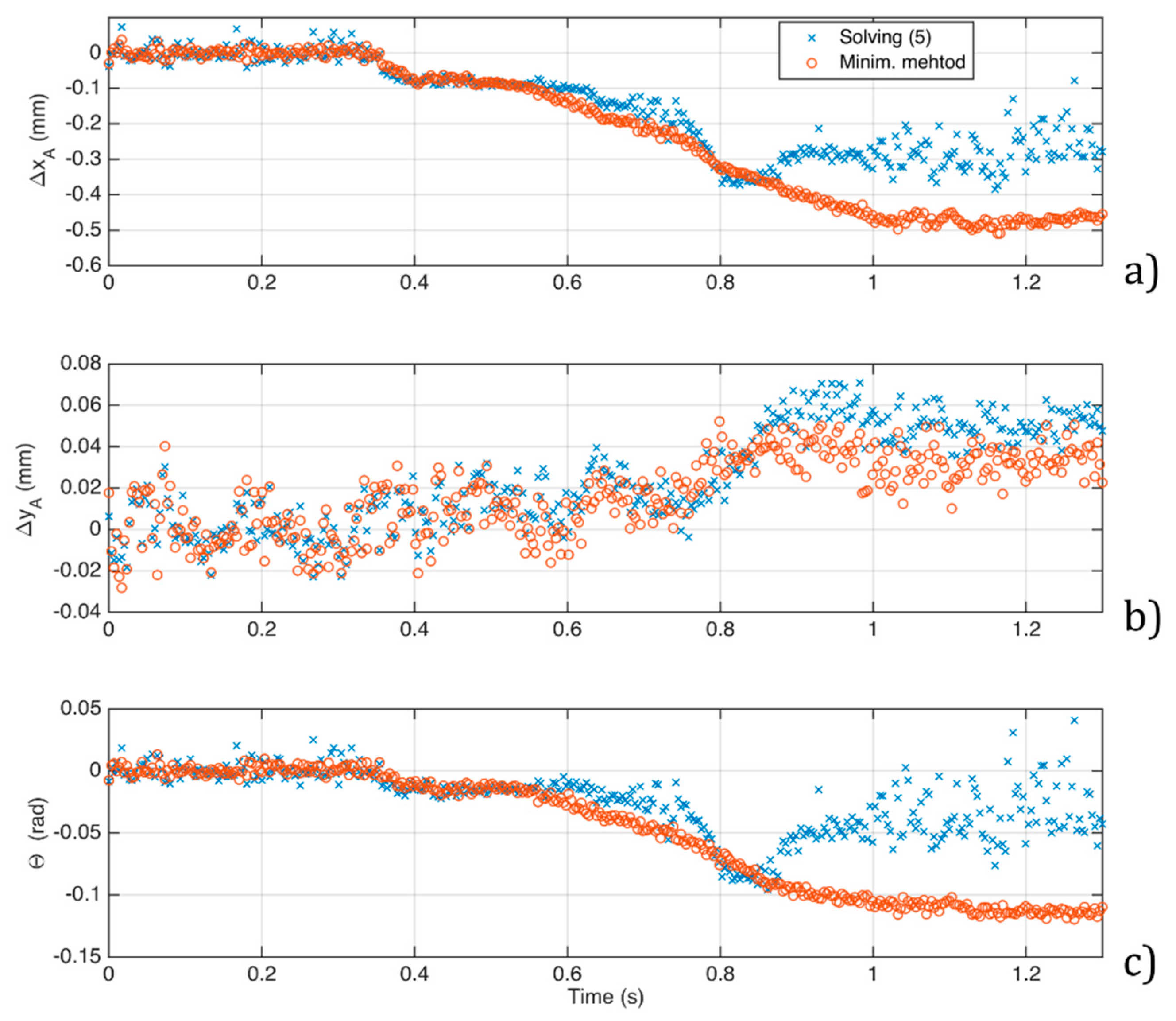
Besides the rotation and the total displacement of points once the applied load has stabilized, the proposed method allows for the instantaneous measurement of these quantities in time, while the load is being transferred from the operator’s hand to the structure and the structure distributes the stresses and suffers strains though the whole structure. The load was applied slowly enough to avoid an additional impact factor in the structure, but fast enough to minimize transference time from the operator’s hand to the structure. Despite this, some small time was spent during this transference and hence both effects (transference load and strain-stresses redistribution) are mixed in the results in time. In Figure 10, we represent the relative displacement of the point A in (a) the x-direction, (b) the y-direction, and (c) the torsional angle computed both separately solving (5) and with the proposed minimization method for the video of Figure 9. Separately solving Equation (5) seems to work well; however, it suddenly provides an inaccurate solution from around 0.8 s. This might be because the errors of both fittings accumulate. The results provided by the minimization method show a smooth behaviour, which allows us to assess the dynamic process. Note that the accuracy of the method (0.01 mm, equivalent to 0.1 px) and the theoretical total displacement in the y-direction (0.07 mm) are of the same order, so the graph in Figure 10b seems wrinklier, and thus the results obtained for this displacement are not reliable.
On the other hand, we have processed the video from the camera recording the contact distance measurer (Figure 11a) in order to obtain the vertical displacement of the beam in time. This measurement can be used to evaluate the results provided by the minimization method in the dynamic process of the deflection. Therefore, we compare it with the results of the proposed technique. Each frame was cropped, binarized, and transformed to polar coordinates around the centre of the clock (Figure 11b). This point was manually selected in the first frame of the sequence. The sum of the intensity values of the columns of that image in polar coordinates is at a minimum where the needle is, so we computed the column of minimum sum and we quantized the number of columns to one hundred discrete levels between 0 and 1, which corresponds to the hundredths of a millimetre (Figure 11c) of the accuracy of the device. Each time a whole lap was performed, we added 1 mm.
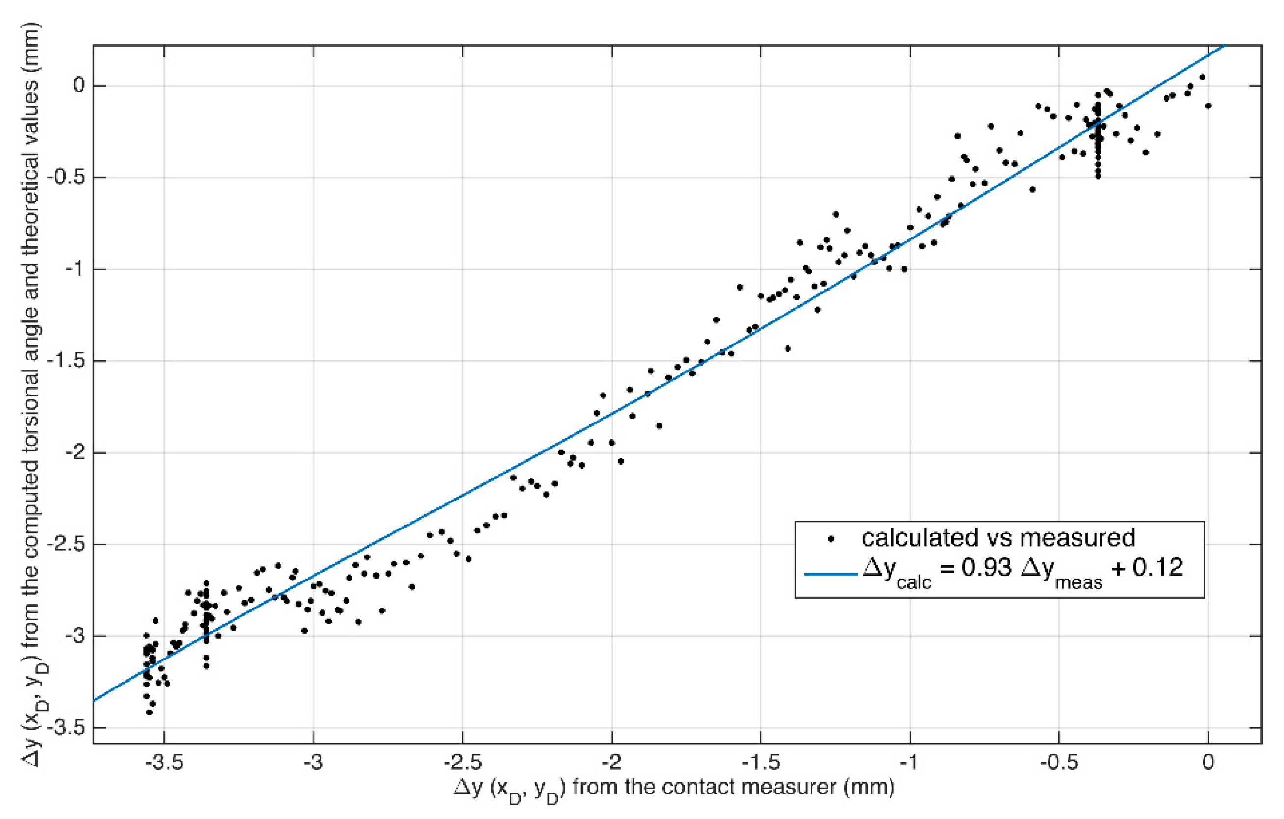
In Figure 12, we have represented the displacement measured with the contact measurer at the point D, versus the torsional angle computed from the orientation of the bisector obtained with the proposed method at the point A, . They are related following (9), which can be simplified into:
We have compared the data from the contact measurer with the angles computed with the proposed technique, , through Equation (10). We imposed the bending values and , the positions and , and the angle , according to the theory, and computed the linear least-square fitting. The results from the fitting are shown in Figure 12, with a p-value <0.05, root mean squared error equal to 0.16 mm, and R = 0.99.
Theoretically, for the point D, the total deflection is . Again, the theoretical value differs from the measurements, if we compare that value with those shown in Figure 12 (around −3.50 mm). This fact made us doubt the accuracy of the parameters used for the theoretical calculations. Probably, some inhomogeneities (density, shape, weldings) in the steel pieces of the structure affect the inertial moments, and therefore the position of the shearing center and/or the torsional angle are not accurately predicted.
5. Discussion and Conclusions
We have presented a targetless noncontact measuring technique that completely locates both the position and orientation of an object describing a trajectory. Two nonparallel segments from the image of the object are used as features to compute, through a simplex minimization method, a location vector that comprises the intersection point and the orientation of the bisector of the angle between them.
We have evaluated the performance of the method both with a numerical simulation and lab experiments that comprised practical applications. The algorithm provides a theoretical mean subpixel accuracy of 0.03 px for the position and 0.02 degrees for the orientation. In the practical application, we reached subpixel accuracy of 0.1 px and 0.04 degrees for the orientation, besides obtaining accuracies of hundredths of deg/s2 in the angular acceleration, and thousandths of deg/s in the angular velocity. The obtained resolutions equal the best ones reported in the literature.
The technique could be used to test the performance of stage motors and engines. In the above example, we were able to distinguish the accelerated phases and the constant velocity phase. The obtained angular velocity value agrees with theoretical one, whereas both angular acceleration values are below the limit of the device. One could also establish the time necessary to reach constant velocity, evaluate the stability of the different phases of the movement (constant velocity, uniformly accelerated, …), and model the acceleration and deceleration stages, etc. The technique has also been useful to measure the change of position in time of a structure under external loads. The instantaneous position is linked with stresses and strains in the structure, but usually only the final position can be measured due to the speed of the process. With this technique, using the fast-enough camera needed, the instant stress-strain process during the structure’s loading can be measured, and additional information about the stress transmission can be obtained.
One of the steps of the algorithm is an image processing block to obtain a binary image with some nonparallel segments. That block is susceptible to being changed depending on the application, thus providing a spread range of use. Indeed, even the condition of the object to remain unaltered in shape and having some nonparallel segments could be relaxed. Of course, it would imply an increase in the uncertainty of the measurement. The technique could be applied to track the translation and rotation of crawling cells in time-lapse video microscopy sequences [4].
We insist on the idea that the algorithm can be adapted and optimized depending on the application. It could be also modified to be addressed to a clinical application, such as image registration [19]. The sequences are processed offline; nevertheless, as future work, we expect to modify the algorithm to perform real-time processing, and then apply the technique to automatic target recognition research.
The method is supported on the a priori knowledge of some structural information, that is that the object extracted from the image does not deform. If we extend that assumption not only to the image plane (XY) but to the Z direction, we could perform three-dimensional tracking. Instead of extracting only two intersecting segments on a plane, we would need three intersecting segments in a three-dimensional space. If the angles between segments do not change in time, we could compute the bisector and use it to track the movement, if the object does not change its shape.
Supplementary Materials
Supplementary File 1Author Contributions
J. Espinosa conceived the main idea, the numerical models, and wrote the paper’s draft. All programming for the theoretical models and the numerical analysis of the experiment was also done by him. J. Perez helped to understand and apply the Nelder–Mead simplex algorithm. The first experiment was conceived and implemented by C. Vazquez. The second experiment was conceived and carried out by B. Ferrer and D. Mas. They also reviewed the final text and calculations.
Conflicts of Interest
The authors declare no conflict of interest. The founding sponsors had no role in the design of the study; in the collection, analyses, or interpretation of data; in the writing of the manuscript; and in the decision to publish the results.
References
- Gonzalez, R.C.; Woods, R.E. Digital Image Processing, 3rd ed.; Prentice Hall: Upper Saddle River, NJ, USA, 2007; ISBN 978-0-13-168728-8. [Google Scholar]
- Lewis, J.P. Fast template matching. Vis. Interface 1995, 95, 120–123. [Google Scholar]
- Lei, X.; Jin, Y.; Guo, J.; Zhu, C. Vibration extraction based on fast NCC algorithm and high-speed camera. Appl. Opt. 2015, 54, 8198–8206. [Google Scholar] [CrossRef] [PubMed]
- Wilson, C.A.; Theriot, J.A. A correlation-based approach to calculate rotation and translation of moving cells. IEEE Trans. Image Process. 2006, 15, 1939–1951. [Google Scholar] [CrossRef] [PubMed]
- Casasent, D.; Psaltis, D. Position, rotation, and scale invariant optical correlation. Appl. Opt. 1976, 15, 1795–1799. [Google Scholar] [CrossRef] [PubMed]
- Reddy, B.S.; Chatterji, B.N. An FFT-based technique for translation, rotation, and scale-invariant image registration. IEEE Trans. Image Process. 1996, 5, 1266–1271. [Google Scholar] [CrossRef] [PubMed]
- Zhou, J.; Shen, W.; Wang, S. Experimental study on torsional behavior of FRC and ECC beams reinforced with GFRP bars. Constr. Build. Mater. 2017, 152, 74–81. [Google Scholar] [CrossRef]
- Joseph, J.; Bhagatji, A.; Singh, K. Content-addressable holographic data storage system for invariant pattern recognition of gray-scale images. Appl. Opt. 2010, 49, 471–478. [Google Scholar] [CrossRef] [PubMed]
- Ge, P.; Li, Q.; Feng, H.; Xu, Z. Image rotation and translation measurement based on double phase-encoded joint transform correlator. Appl. Opt. 2011, 50, 5235–5242. [Google Scholar] [CrossRef] [PubMed]
- Erturk, S. Translation, rotation and scale stabilisation of image sequences. Electron. Lett. 2003, 39, 1245–1246. [Google Scholar] [CrossRef]
- Shaik, J.S.; Iftekharuddin, K.M. Detection and tracking of rotated and scaled targets by use of Hilbert-wavelet transform. Appl. Opt. 2003, 42, 4718–4735. [Google Scholar] [CrossRef] [PubMed]
- Zheng, T.; Cao, L.; He, Q.; Jin, G. Image rotation measurement in scene matching based on holographic optical correlator. Appl. Opt. 2013, 52, 2841–2848. [Google Scholar] [CrossRef] [PubMed]
- Jahne, B. Practical Handbook on Image Processing for Scientific and Technical Applications, 2nd ed.; CRC Press: Boca Raton, FL, USA, 2004. [Google Scholar]
- Espinosa, J.; Perez, J.; Ferrer, B.; Mas, D. Method for targetless tracking subpixel in-plane movements. Appl. Opt. 2015, 54, 7760–7765. [Google Scholar] [CrossRef] [PubMed] [Green Version]
- Lagarias, J.; Reeds, J.; Wright, M.; Wright, P. Convergence properties of the nelder—Mead simplex method in low dimensions. SIAM J. Optim. 1998, 9, 112–147. [Google Scholar] [CrossRef]
- Strang, G. Introduction to Applied Mathematics; Wellesley-Cambridge Press: Wellesley, MA, USA, 1986; ISBN 978-0-9614088-0-0. [Google Scholar]
- Gere, J.M. Mechanics of Materials, 6th ed.; Brooks/Cole—Thomson Learning: Belmont, CA, USA, 2004. [Google Scholar]
- Canny, J. A computational approach to edge detection. IEEE Trans. Pattern Anal. Mach. Intell. 1986, PAMI-8, 679–698. [Google Scholar] [CrossRef] [PubMed]
- Hutton, B.F.; Braun, M. Software for image registration: Algorithms, accuracy, efficacy. Semin. Nucl. Med. 2003, 33, 180–192. [Google Scholar] [CrossRef] [PubMed]
Figure 1.
Two nonparallel segments (blue lines), best fitting straight lines to each segment (dashed blue lines), intersection (xc, xc), and bisectors (red lines).
Figure 1.
Two nonparallel segments (blue lines), best fitting straight lines to each segment (dashed blue lines), intersection (xc, xc), and bisectors (red lines).

Figure 2.
Cartesian coordinates system formed by bisectors centred at the intersection.
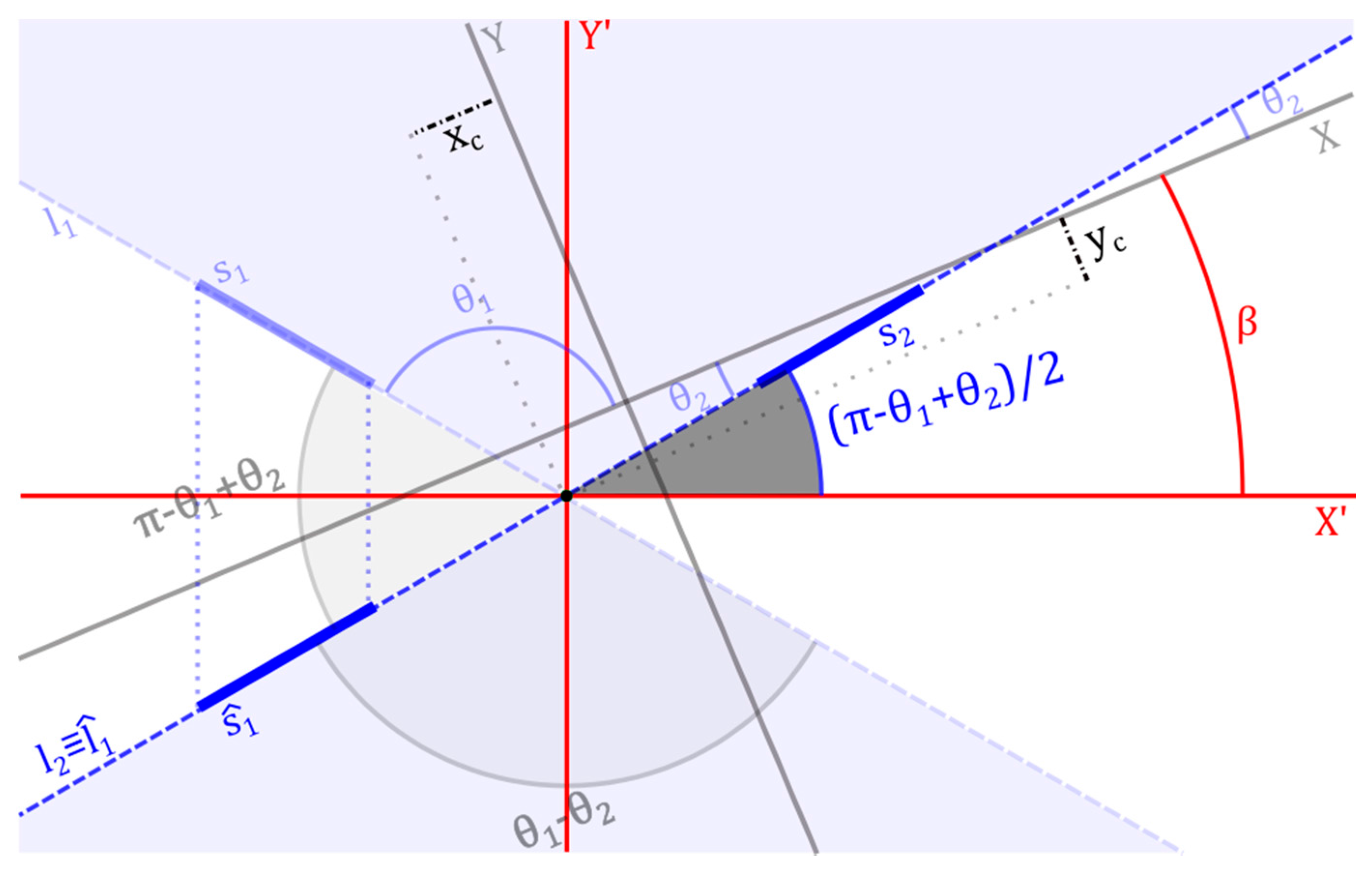
Figure 3.
Flow chart for the algorithm.
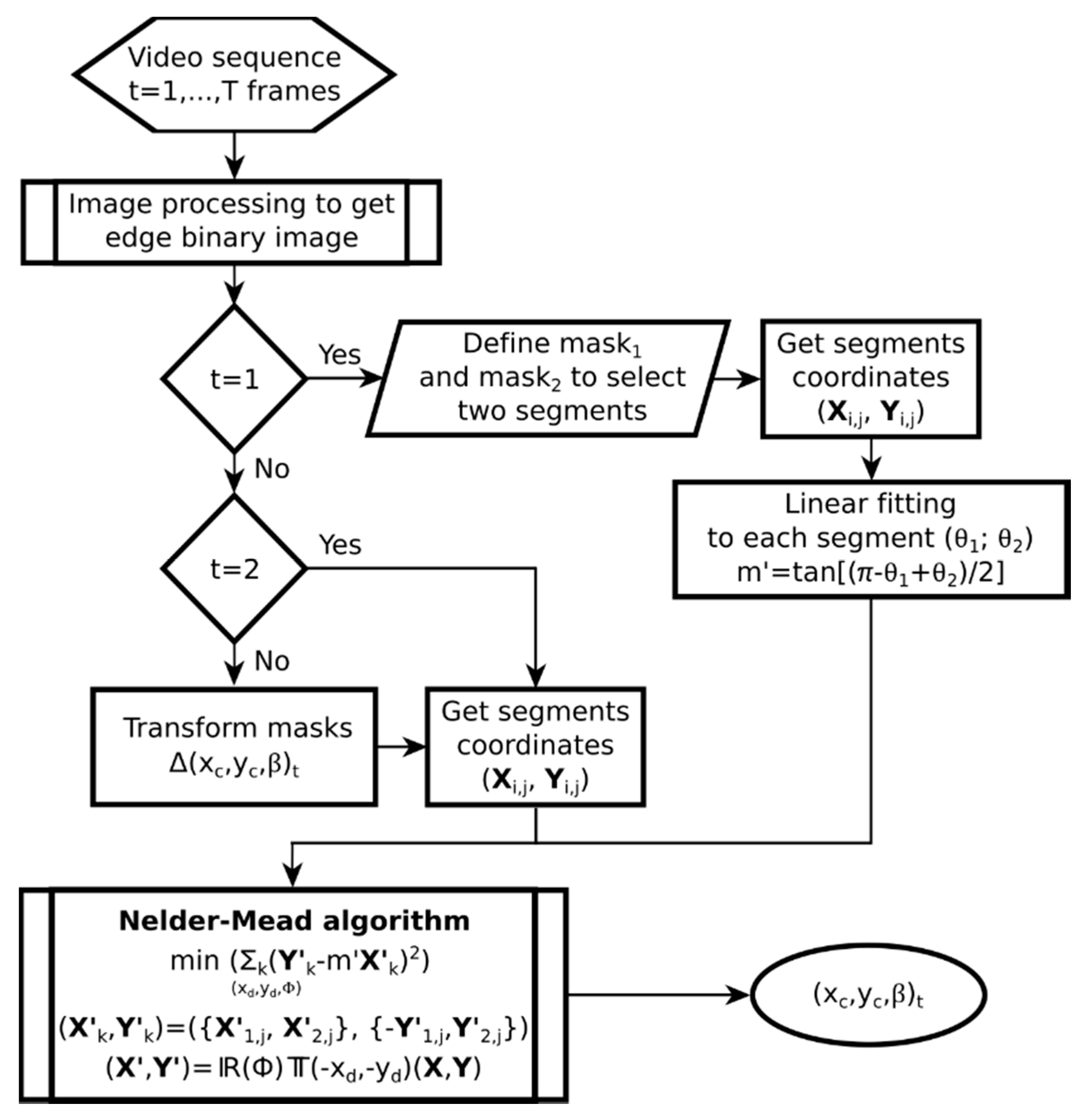
Figure 4.
Segments (white) extracted from a rhombus and the obtained bisector (pink line), its orientation and the intersection point (pink cross) together with the theoretical intersection (green cross) and rotation centre (red circle).
Figure 4.
Segments (white) extracted from a rhombus and the obtained bisector (pink line), its orientation and the intersection point (pink cross) together with the theoretical intersection (green cross) and rotation centre (red circle).
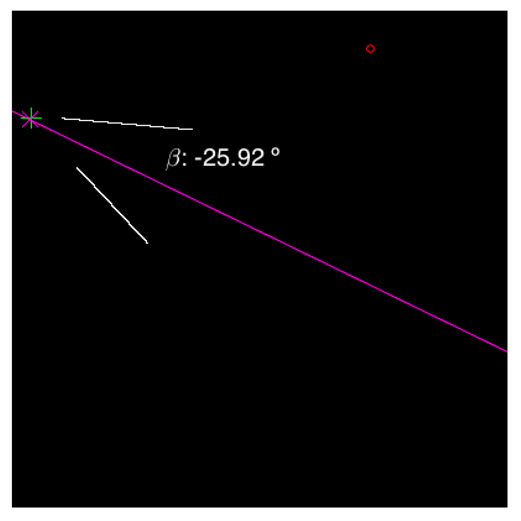
Figure 5.
Quotient between the computed and the theoretical parameters of the location vector (xc (crosses), yc (squares), β (circles)) for the frames of the above simulated sequence.
Figure 5.
Quotient between the computed and the theoretical parameters of the location vector (xc (crosses), yc (squares), β (circles)) for the frames of the above simulated sequence.

Figure 6.
Scheme of the lab experiment to measure the torsion and bending of a cantilever steel beam. The units of distances drawn are millimeters.
Figure 6.
Scheme of the lab experiment to measure the torsion and bending of a cantilever steel beam. The units of distances drawn are millimeters.

Figure 7.
The image of the object fixed to the rotation stage was (a) cropped, (b) quantized, (c) edge extracted, (d) and removed of small objects, successively. From the final step, we selected two areas from where the segments were extracted. (e) Frame of the recorded video (see Visualization 2) of the object in the rotation stage together with the selected segments in blue and the computed intersection.

Figure 8.
Variation in time of the orientation of the computed bisector for the selected segments from the rotation stage experiment. The curve was divided into three, approximately distinguishing between the linear (blue circles) and nonlinear parts (red circles). The blue line and the red dashed lines represent the best curve fitting to each part.

Figure 9.
Frame of the recorded video (see Visualization 3) of the U-shaped beam during the experiment with the selected segments in blue, the intersection (red square), and the computed bisector (pink).
Figure 9.
Frame of the recorded video (see Visualization 3) of the U-shaped beam during the experiment with the selected segments in blue, the intersection (red square), and the computed bisector (pink).
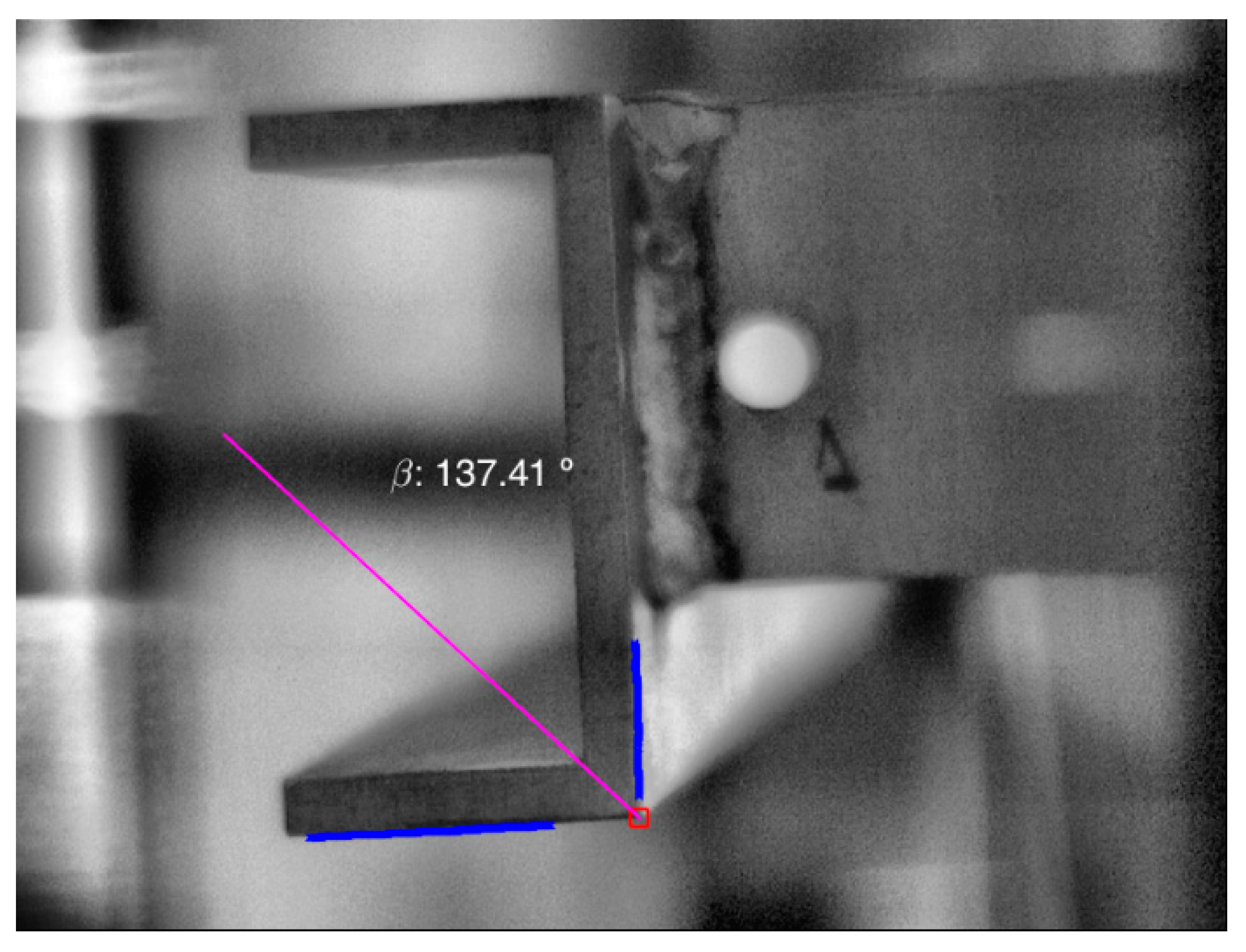
Figure 10.
(a) x-displacements at A, (b) y-displacements at A, and (c) torsional angle computed using the proposed minimization method (red) and separately solving Equation (5) (blue).
Figure 10.
(a) x-displacements at A, (b) y-displacements at A, and (c) torsional angle computed using the proposed minimization method (red) and separately solving Equation (5) (blue).

Figure 11.
(a) Region of interest (ROI) of a frame of the recorded sequence by the camera focusing on the contact measurer. (b) Binarized and Cartesian-to-Polar transformed image of the ROI. (c) Sum of intensity of the pixels in Figure 11b by columns. Columns have previously been discretized to cover the range from 0 to 1 mm with steps of 0.01 mm, according to the accuracy of the device.
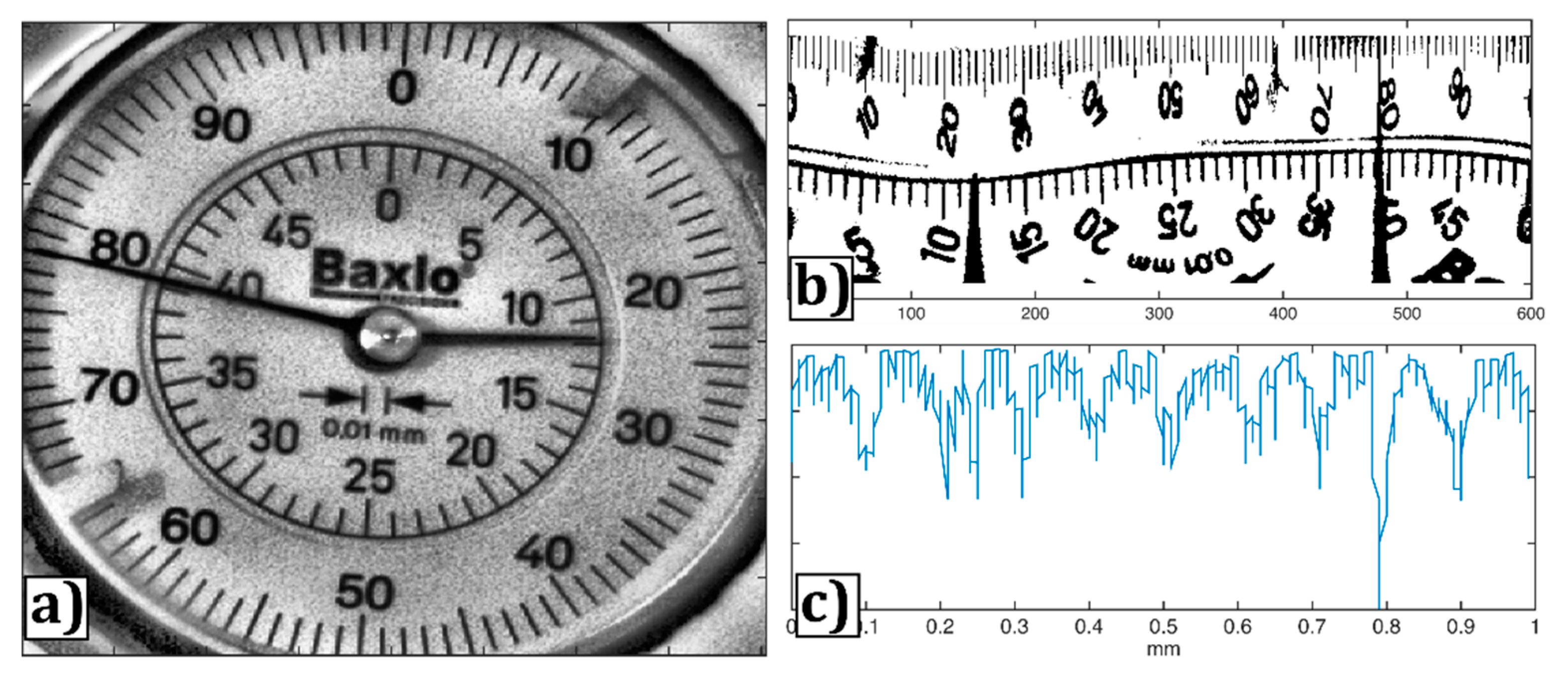
Figure 12.
Vertical displacement computed from Equation (10) with theoretical values for ∆yB, rD, yD, and γD, and the torsional angle obtained with the proposed method versus the vertical displacement measured with the contact measurer at the point D (black dots). The blue line represents the linear least-square fitting.

Table 1.
Horizontal and vertical distances and torsional angle obtained from the location vector components computed using different methods for the experiment in Figure 9, and the theoretical values. Errors are obtained as standard deviation of the computed component of the last 50 frames of the sequence, when the system is static.
| Minim. Method | Solving (5) | Theoretical | |
|---|---|---|---|
| −0.47 ± 0.01 | −0.25 ± 0.06 | −0.5698 | |
| 0.033 ± 0.007 | 0.049 ± 0.006 | 0.0591 | |
| −0.0187 ± 0.0004 | −0.005 ± 0.004 | −0.0228 1 |
1 Distances in millimeters and angles in radians.
© 2017 by the authors. Licensee MDPI, Basel, Switzerland. This article is an open access article distributed under the terms and conditions of the Creative Commons Attribution (CC BY) license (http://creativecommons.org/licenses/by/4.0/).
Share and Cite
MDPI and ACS Style
Espinosa, J.; Pérez, J.; Ferrer, B.; Vázquez, C.; Mas, D. Bisector-Based Tracking of In Plane Subpixel Translations and Rotations. Appl. Sci. 2017, 7, 835. https://doi.org/10.3390/app7080835
AMA Style
Espinosa J, Pérez J, Ferrer B, Vázquez C, Mas D. Bisector-Based Tracking of In Plane Subpixel Translations and Rotations. Applied Sciences. 2017; 7(8):835. https://doi.org/10.3390/app7080835
Chicago/Turabian StyleEspinosa, Julián, Jorge Pérez, Belén Ferrer, Carmen Vázquez, and David Mas. 2017. "Bisector-Based Tracking of In Plane Subpixel Translations and Rotations" Applied Sciences 7, no. 8: 835. https://doi.org/10.3390/app7080835
Note that from the first issue of 2016, this journal uses article numbers instead of page numbers. See further details here.