Article

A Novel Reactive Power Optimization in Distribution Network Based on Typical Scenarios Partitioning and Load Distribution Matching Method

1
College of Information and Electrical Engineering, China Agricultural University, Beijing 100083, China
2
Power Distribution Research Department, China Electric Power Research Institute, Beijing 100192, China
*
Authors to whom correspondence should be addressed.
Appl. Sci. 2017, 7(8), 787; https://doi.org/10.3390/app7080787
Submission received: 8 June 2017 / Revised: 25 July 2017 / Accepted: 31 July 2017 / Published: 3 August 2017
(This article belongs to the Section Mechanical Engineering)

Abstract

:

Featured Application

This work is a prospective study on reactive power optimization based on the background of big data, which is supported by Science and Technology Project of State Grid Corporation of China (SGCC) (EPRIPDKJ (2015) 1495), and Beijing Natural Science Foundation (3172039). The research results will be applied in demonstration applications of SGCC in the future.

Abstract

This paper proposed an entropy weight optimum seeking method (EWOSM) based on the typical scenarios partitioning and load distribution matching, to solve the reactive power optimization problem in distribution network under the background of big data. Firstly, the mathematic model of reactive power optimization is provided to analyze the relationship between the data source and the optimization schemes in distribution network, which illustrate the feasibility of using large amount of historical data to solve reactive power optimization. Then, the typical scenarios partitioning method and load distribution matching method are presented, which can select out some loads that have the same or similar distributions with the load to be optimized from historical database rapidly, and the corresponding historical optimization schemes are used as the alternatives. As the reactive power optimization is a multi-objective problem, the multi-attribute decision making method based on entropy weight method is used to select out the optimal scheme from the alternatives. The objective weights of evaluation indexes are determined by entropy weight method, and then the multi-attribute decision making problem is transformed to a single attribute decision making problem. Finally, the proposed method is tested on several systems with different scales and compared with existing methods to prove the validity and superiority.

1. Introduction

Reactive power optimization is an effective means to ensure the safe and economic operation of power system. The reasonable reactive power distribution can reduce the network loss [1,2], improve the voltage quality [3,4], and maintain the normal operation of the power grid. Reactive power optimization is a nonlinear mixed integer programming problem with multiple objectives, and generally, the solution of existing methods is to make hypothesis and simplifications of the optimal model, and then solve it with iterative optimization. The optimization algorithm can be roughly divided into two types: the traditional optimization method such as interior point method [5], sequential quadratic programming [6], and artificial intelligence algorithms such as genetic algorithm [7], particle swarm algorithm [8], and multi-agent technology [9]. With a large number of distributed generators [10,11,12], energy storages and demand side response control equipment [13,14,15,16] access to distribution network, the number of control variables in reactive power optimization increased significantly, while the convergence cannot be guaranteed and the computation time of traditional mathematical methods increased. The results of artificial intelligence algorithms are instable and easy to fall into local optimum.
In order to improve the convergence, accuracy and computing speed of reactive power optimization, the existing literature mainly studied on the simplification of the model and the improvement of the algorithm. Literature [17] proposed a method to optimally set the reactive power contributions of distributed energy resources present in distribution systems with the goal of regulating bus voltages, then the reactive power optimization was modeled as a convex quadratic program and solved based on the alternating direction method of multipliers efficiently. Literature [18] proposed an advanced loss reduction approach to achieve the optimal control coordination among multiple capacitors and DERs. The proposed approach and solution were developed on the basis of the detailed multi-phase distribution network modeling and the state-of-the-art optimization technology. The effectiveness of the proposed approach was demonstrated on practical utility distribution circuits with varying degree of unbalance and model complexity. Literature [19] presented a mixed-integer linear programming model to solve the simultaneous transmission network expansion planning and reactive power planning problem. The proposed model considered reactive power, off-nominal bus voltage magnitudes, power losses, multistage expansion, and security constraints. The use of a mixed-integer linear programming (MILP) model guaranteed convergence to optimality by using existing classical optimization methods. Although the above research has improved the efficiency and convergence of reactive power optimization, it has not been separated from the limitations of the traditional algorithm model and iterative optimization.
In recent years, big data technology has been paid more and more attention by experts and scholars in various fields. The basic idea of big data is to guide the system operation or production practice in the future by means of analyzing a large amount of data generated from practice or production system, finding a certain law, and establishing the corresponding data model [20,21]. The distribution network contains many nodes, the database has accumulated a lot of historical data, and the power load showed a certain cyclical characteristics, which make it possible to apply the theory and method of big data to reactive power optimization in distribution network.
At present, the research and application of big data in distribution network is still in the initial stages. The relevant research focuses on multi-source data fusion and data storage technology [22,23], application requirements and typical scene analysis [24,25,26], running state analysis [27,28,29] and other fields, and it has made some achievements. In this paper, the method of modeling and analysis of big data is introduced into the field of reactive power optimization in distribution network.
Based on the above background, an entropy weight optimum seeking method (EWOSM) is proposed to solve the reactive power optimization in distribution network. The method contains two steps. Firstly, typical load scenarios and topology scenarios are established based on historical data, and a load distribution matching method based on Pauta criterion is proposed to select out some alternatives from the historical database. Secondly, three evaluation indexes including the network loss, node voltage offset and static voltage stability index are used to analyze and evaluate the alternatives, and entropy weight method [30,31,32] is used to choose the optimal control scheme from the alternatives.
The remainder of the paper is organized as follows. The method of typical scenarios partitioning and load distribution matching are presented in Section 2. And Section 3 presents the reactive power optimization method based on entropy weight method. Case simulation with different systems and results comparisons are provided in Section 4. Section 5 is the summary and presents the conclusions.

2. The Method of Typical Scenarios Partitioning and Load Distribution Matching

2.1. Relationship between the Data Source and the Optimal Schemes in Reactive Power Optimization

The database in distribution network has accumulated a large amount of historical data, which comes from different systems, such as SCADA (Supervisory Control and Data Acquisition), GIS (Geographic Information System) and EMS (Energy Management System). It also can be divided into operational monitoring data, marketing data, and management data according to the use of data. Besides, part of the data is well-structured, but more data is unstructured or semi-structured. Facing such a large amount of multi-source and heterogeneous data, it is necessary to consider how to select out the effective data and make fully use of it to solve reactive power optimization problem. Therefore, data fusion and data cleaning should be performed to make all the data well-structured firstly [33,34]; then, the mathematic model of reactive power optimization is provided to analyze the relationship between the data source and the optimal schemes, which can guide us to find out the data that have a decisive effect on reactive power optimization.
Reactive power optimization is a multi-objective programming problem, and generally the network loss, the node voltage offset and the minimum module-eigenvalue of the Jacobian matrix are chosen as the objective functions to evaluate the economy and security of the system. The minimum module-eigenvalue can measure the static voltage stability of the system; the smaller the value is, the more unstable the system is, and the value will decrease to 0 if the voltage collapse occurs. The formulas of the objective function are expressed as follows:
min f = w 1 f 1 + w 2 f 2 + w 3 f 3
f 1 = i , j = 1 n G i j ( V i 2 + V j 2 2 V i V j cos θ i j )
f 2 = i = 1 n ( V i V i B Δ V i max ) 2
f 3 = min ( | e i g ( J ) | )
where f is the objective function; f1, f2 and f3 are respectively the network loss, the node voltage offset and the minimum module-eigenvalue; w1, w2 and w3 are the corresponding weight of f1, f2 and f3, and w1 + w2 + w3 = 1; Vi and Vj are the voltage amplitude of node i and node j; Gij and θij are respectively the conductance and voltage phase angle difference between node i and node j, and particularly ij; n is the number of nodes in the system; ViB is the ideal voltage amplitude of node i, whose value is usually 1.0 (p.u.); ΔVimax is the maximum allowable voltage offset of node i, which is generally ±7% in the distribution network; J is the Jacobian matrix while the power flow is converged; and eig (J) is the eigenvalue of matrix J.
The constraint of the reactive power optimization model contains power balance constraints, voltage constraints and control variables constraints. The power balance constraints are as follows:
P G i P L i V i j = 1 n V j ( G i j cos θ i j + B i j sin θ i j ) = 0
Q G i Q L i V i j = 1 n V j ( G i j sin θ i j B i j cos θ i j ) = 0
where PGi and QGi represent the active and reactive power of node i; PLi and QLi represent the active and reactive load of node i; Bij represents the susceptance between node i and node j.
The voltage and the control variables constraints are expressed as follows:
V i , min V i V i , max
Q c i q = K c i q q c i q , i q = 1 , , n q
T i T = 1 + K T i T Δ T i T , i T = 1 , , n T
where Vi,min and Vi,max represent the upper and lower voltage bounds of node i respectively; nq and nT are respectively the number of capacitor compensation nodes and transformer nodes; if the capacitors are equal grouping and the single capacity is qciq, Qciq is the compensation capacity of node iq with Kciq groups put into operation; T i T is the ratio of transformer with the tap position K T i T and the minimum adjustment Δ T i T .
As expressed in Equations (1)–(4), the objective function f can be expressed as a function of the system active load P, reactive load Q, the capacitor compensation capacity Qc and the transformer tap T, which can be expressed as follows:
f = F ( P , Q , Q c , T )
where F(·) expresses a mapping relation from P, Q, Qc and T to the optimal objective function.
Generally, the reactive power control scheme in distribution network consists of compensation capacity Qc and transformer tap T, which are determined by the load level and load distribution in each node while the network topology remains unchanged. Besides, reactive load is dependent upon the existence of active load, so it can be obtained by power factor. Therefore, Equation (10) can be simplified as follows:
( Q c , T ) = g ( P 1 , P 2 , , P n ; Q 1 , Q 2 , , Q n )
where g(·) expresses a mapping relation from load distribution to reactive power control scheme; (P1, …, Pn) and (Q1, …, Qn) respectively express the active power load and reactive power load distribution in different nodes.
Since the compensation capacity of capacitor and the transformer tap are both finite discrete variables, the number of reactive power control schemes is limited. Though power load is a continuous variable and has some randomness, it appears a strong regularity and periodicity; and the optimal reactive compensation scheme remains the same in a certain range of load fluctuation. Therefore, while the amount of power load data and load distribution patterns that accumulated in the historical database is large enough, and assume that all historical control schemes are optimal, the corresponding control schemes of the existing load distributions are all contained in the database.
Therefore, if the reactive power optimization is carried out for a certain time in the future, the similar network topologies, load distributions and corresponding control schemes are selected out from the historical database, and then the optimal control scheme is among the schemes. This paper is to solve the problem that how to find out the optimal plan from the historical database.

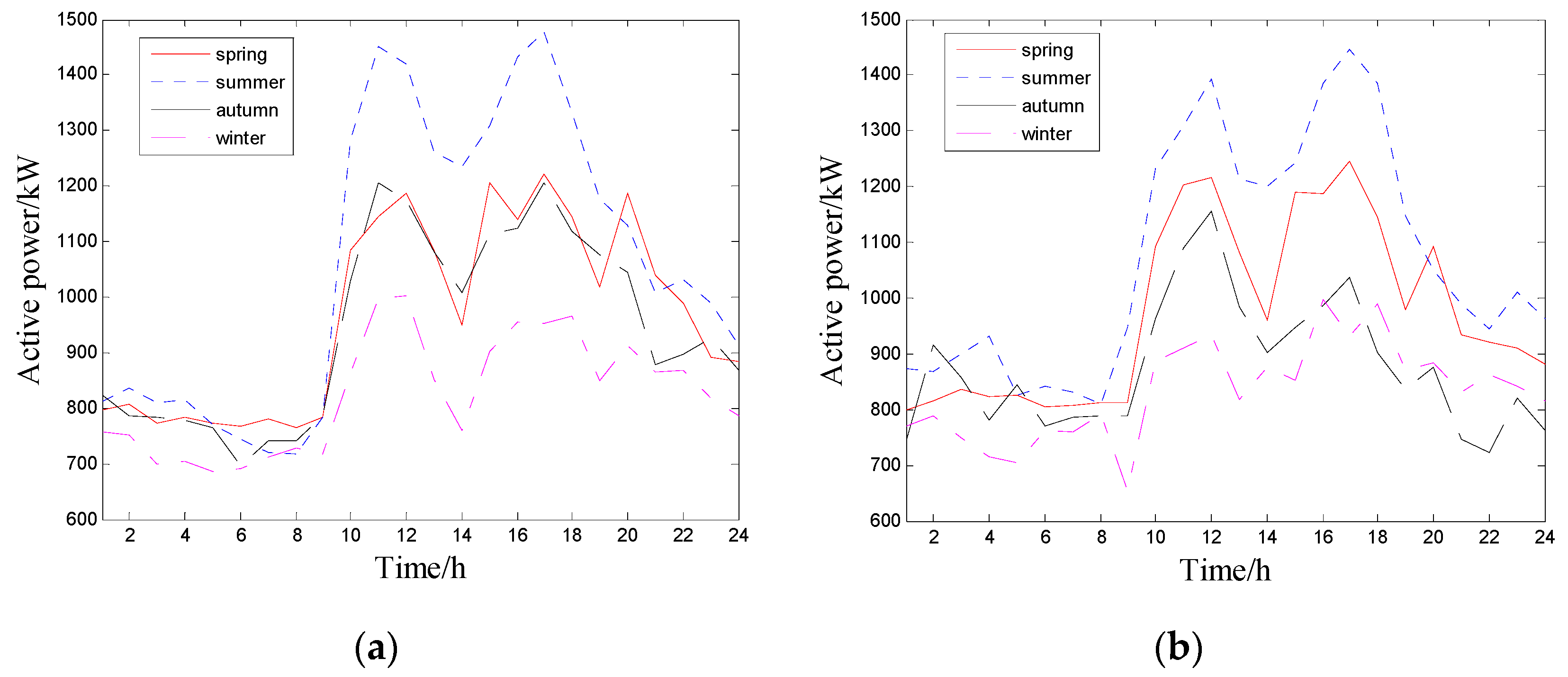
2.2. The Method of Typical Scenarios Partitioning

In the previous section, it is concluded that the control scheme of reactive power in distribution network is determined by the network topology and load distribution. Then, how to make fully and effectively use of the two types of data in historical database has become the key to solve reactive power optimization problem. This paper presented a typical scenarios partitioning method, containing typical topology scenarios partitioning and typical load scenarios partitioning.
Firstly, typical topology scenarios partitioning method is presented. The change of topology in distribution network is achieved by the cooperation of section switches and tie switches. Although the combination of different switch states can produce many kinds of network topologies, it can be seen from the historical operating data that the difference of the duration of different network topologies in one year is obvious, and the number of typical topologies that has long duration is limited. Therefore, select topologies that has long duration in historical database as the typical topology scenarios, and other topologies are treated as special scenarios.
Secondly, the method of typical load scenarios partitioning is as follows. For some load that have strong regularity and change smoothly, the load fluctuates around its typical load curve during a specific operating cycle; while the data quantity is large enough, this type of load obeys a normal distribution approximately around its typical load curve in a specific scenario in statistically, so the similar load distributions can be found in the typical load scenario corresponding to the load distribution to be optimized. As it appears different load characteristics in different seasons, weekdays and weekends, it can be simply divided into eight typical load scenarios preliminarily, that is, weekdays and weekend in four seasons. Besides, different types of load are affected by different factors, so the eight typical load scenarios can be further refined according to the weather, holidays and other factors, to increase the number of typical scenarios. For example, typical scenarios of residential load in summer can be further subdivided based on temperature and humidity; national legal holidays also have great influence on the commercial load, so it can be subdivided into the scenario of Spring Festival, May Day, National day and other scenarios. The refinement of typical load scenarios can not only improve the accuracy of load distribution matching, but also improve the computing time of the method. The typical daily load curves of the eight scenarios in a certain region are shown in Figure 1.

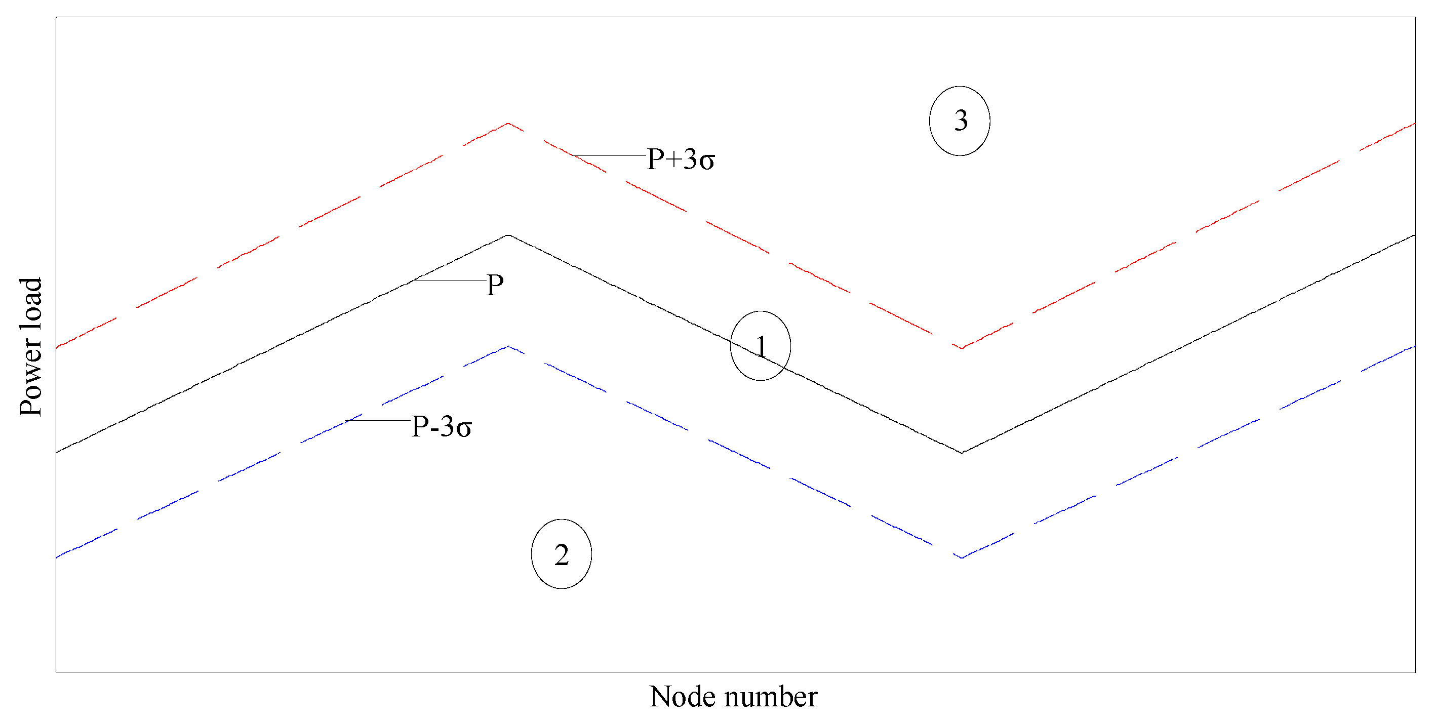
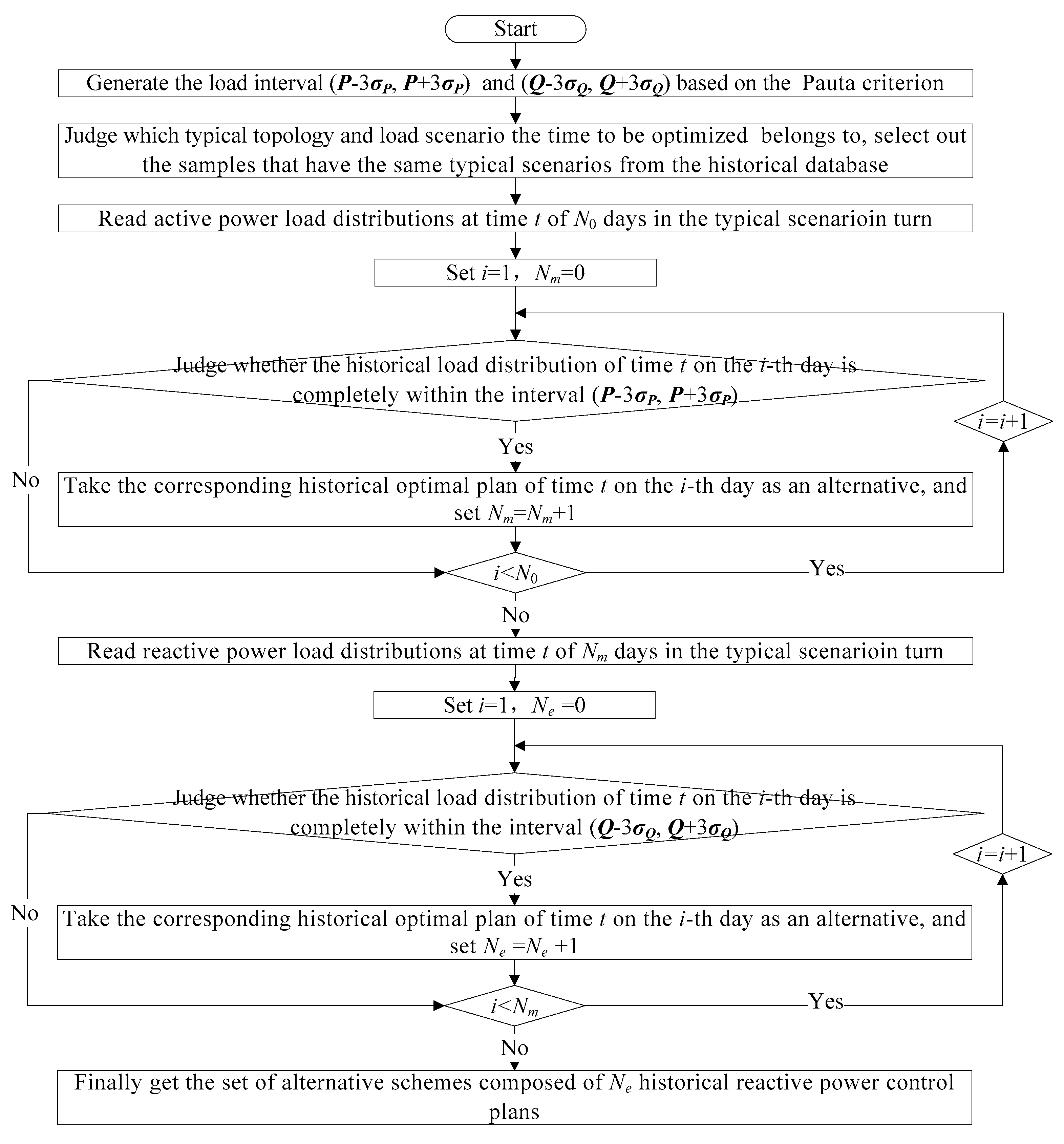
2.3. The Method of Load Distribution Matching

This paper proposed a load distribution matching method, which can quickly find out the load that has the similar distribution with the load to be optimized from massive historical data, and the corresponding control schemes are also selected out. While the power flow of time t in a certain day is to be reactive power optimized, the first step is to select out the samples that both have the same topology scenario and load distribution scenario with the load at time t, and the samples form a set. Secondly, load distribution matching method is implemented with the sample set, and then a smaller sample set is formed, which contains the optimal scheme.
Assume that there are N0 days in the historical database that has the same topology scenario and load scenario to the time t; then match the load distribution at time t of the N0 days with the moment to be optimized in turn, and select out the load that has the similar distribution with the time t. Suppose that there are Ne similar load distributions are selected out, then the corresponding historical optimal schemes form the alternative set.
It is necessary to make a matching rule for the load distribution matching. If a load distribution obeys the rule, it can judge that the load distribution is similar to the moment to be optimized, and its corresponding historical optimal plan can be an alternative. In the Pauta criterion of statistics, while the amount of statistical data is large enough, the probability of the value of the random variable that subject to the normal distribution N ~(μ,σ2) beyond μ ± 3σ is 0.27%, which is considered a small probability event and almost impossible happened in mathematics.
The Pauta criterion is applied to the load distribution matching in this paper. In a system with n nodes, generate two load intervals (P − 3σP, P + 3σP) and (Q − 3σQ, Q + 3σQ), where the mean values are the load to be optimized in each node P = (P1, …, Pn) and Q = (Q1, …, Qn); the variance values are σP2 and σQ2; σP = (σP1, …, σPn) and σQ = (σQ1, …, σQn) are empirical value, which can be calculated with large amount of historical load in different typical scenarios. Take the active power load as an example to illustrate the specific matching process, the active load is divided into three regions by the interval (P − 3σP, P + 3σP), which is shown in Figure 2.
Read load distributions in the typical scenario from the historical database in turn. And if a load distribution is completely within the interval (P − 3σP, P + 3σP), that is, within the Region 1 in Figure 2, take the corresponding historical optimal plan as an alternative; otherwise, the corresponding historical plan cannot be used. After the active power load distribution matching is finished and Nm historical load are selected out, reactive power load distribution matching is also carried out with the Nm historical load.
In summary, if the reactive load optimization is carried out for the load at time t, the process of the load distribution matching is shown in Figure 3, and the final result is a set of alternative schemes composed of Ne historical reactive power control plans.
As the method proposed in this paper is dependent on the historical data, it is suitable for the system that the load changes smoothly and the historical data accumulates enough. In the system with frequently load changing or little historical data, maybe there is no load in the interval (P − 3σP, P + 3σP) to be matched or the number of matched load samples is little. There are two solutions in this case. The first one is simulation off-line, generate a number of load distributions in the interval (P − 3σP, P + 3σP) randomly, and conventional method is used for reactive power optimization of each load distribution respectively; the historical database is extended in this way, and then the proposed method can be used. The second solution is that conventional method is directly used for reactive power optimization and the optimal results are saved into the database; while enough load data are accumulated in the database, the proposed method can be used.

3. Reactive Power Optimization in Distribution Network Based on EWOSM

3.1. Introduction to Multi-Attribute Decision Making Problem Based on Entropy Weight Method

While selecting the optimal control scheme from alternatives, several reactive power optimization evaluation indexes should be considered comprehensively, including the network loss, voltage offset, power factor and so on. Therefore, it is a multi-attribute decision making problem, which is also called multiple objective decision making with finite alternatives. It is a decision making problem that select the optimal scheme from alternatives or schedule the alternatives ranking with the consideration of multiple attributes. Entropy weight method based on information entropy can solve the problem. The objective weights of multiple attribute indexes are determined by information entropy calculated from alternatives, and then the best scheme is selected out.
The concept of entropy is derived from thermodynamics and it is a physical quantity that reflecting the directivity of natural thermal processes in initially. Then information entropy is put forward with the development of related research, which opens up a new way for quantitative decision method. In information theory, the amount and quality of information obtained in decision-making is an important factor to determine the accuracy and reliability of final decision. Exactly, entropy is a good measure for useful information provided by data.
In the multi-attribute decision making problem with M evaluation indexes and N alternatives, the evaluation index matrix is expressed as follows:
Y = [ y 11 y 12 y 1 N y 21 y 22 y 2 N y M 1 y M 2 y M N ]
where yij is the value of the i-th evaluation index at the j-th alternative.
Matrix R = {rij} is got with the standardized of matrix Y. The greater the value of the element in matrix R is, the better the evaluation effect is, so all evaluation indexes should be standardized according to this regulation. For the evaluation index that smaller value has better evaluation effect should be standardized with Equation (13), and conversely with Equation (14).
r i j = max j { y i j } y i j max j { y i j } min j { y i j }
r i j = y i j min j { y i j } max j { y i j } min j { y i j }
where max j { y i j } and min j { y i j } are respectively the maximum and minimum value of the i-th row in matrix Y. The maximum value of the elements in matrix R is 1 and minimum is 0, that is, 0 ≤ rij ≤ 1, where i = 1, …, M; j = 1, …, N.
Calculate the proportion pij that evaluation index rij on the i-th index according to Equation (15), where rij is the i-th evaluation index of the j-th alternative.
p i j = r i j / j = 1 N r i j
And the entropy of the i-th evaluation index is expressed as follows [35]:
H i = k j = 1 N p i j ln p i j
where pij × lnpij = 0 if pij = 0; and k = 1/ln N in order to make it meet the constrain that 0 ≤ Hi ≤ 1.
Entropy is a measure of uncertainty, and the smaller the entropy value is, the more effective the information corresponding to the evaluation index is. Therefore, the entropy weight wi of the i-th index is shown as follows:
w i = 1 H i M i = 1 M H i
After the entropy weight of each evaluation index is determined, the multi-attribute decision making is transformed into a single attribute decision making problem; and then the optimal scheme can be selected from the alternatives.

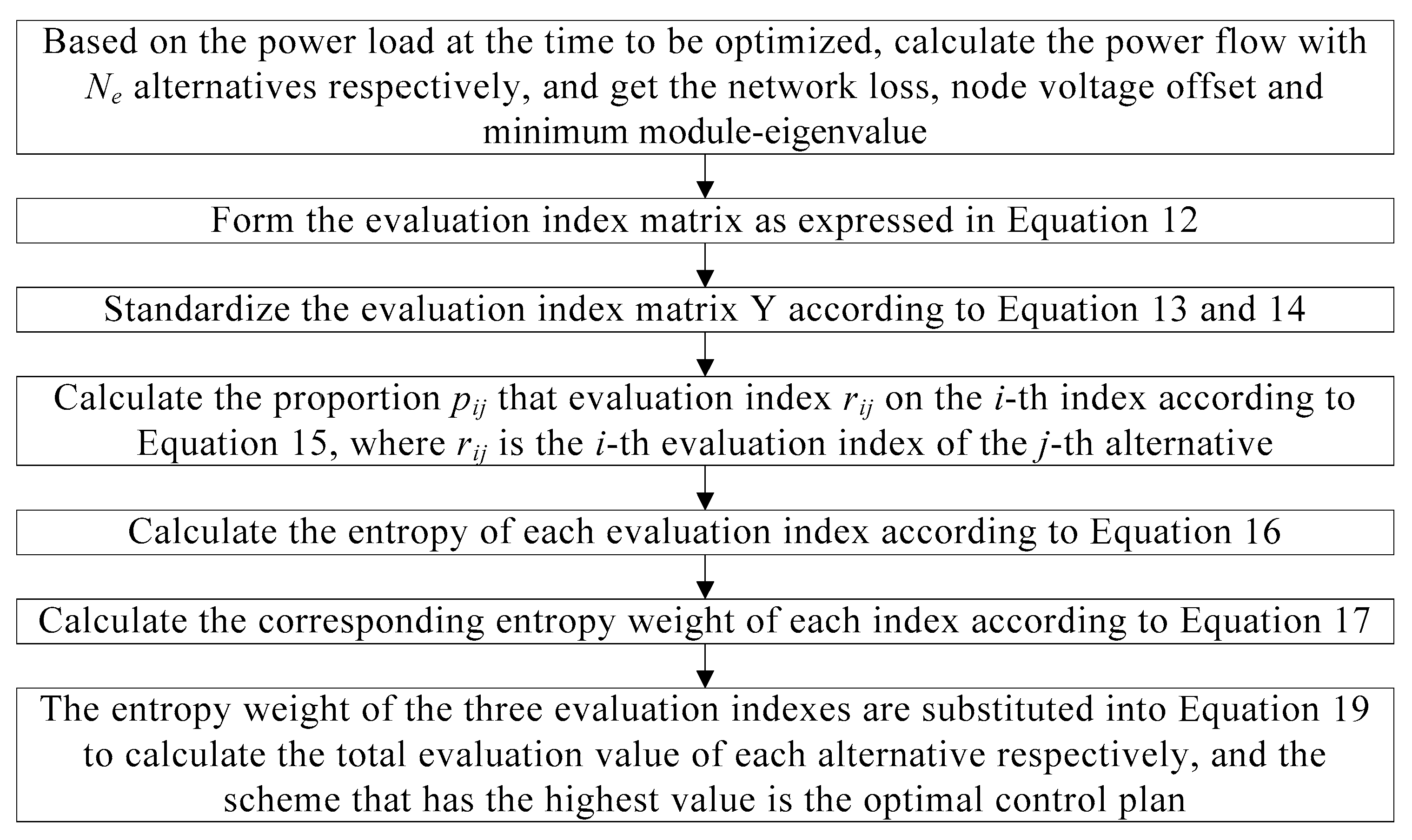
3.2. Specific Steps of EWOSM

The proposed EWOSM contains two procedures. Firstly, typical scenarios partitioning and load distribution matching method is used and select out Ne alternative schemes from historical database. Secondly, select the optimal scheme from alternatives with the entropy weight method, and the specific steps are expressed as follows.
Step 1: Based on the power load at the time to be optimized, calculate the power flow with Ne alternatives respectively and the results of power flow must be checked according to Equations (5)–(9) to ensure the constraints are satisfied. If the constraints are not met, the corresponding alternative control scheme should be removed. Besides, three indexes containing the network loss, the node voltage offset and the minimum module-eigenvalue of the Jacobian matrix are used to evaluate the control effect of each alternative, and the three indexes are presented by y1, y2 and y3.
Step 2: This is a multi-attribute decision-making problem with 3 evaluation indexes and Ne alternatives, and the evaluation index matrix is formed as expressed in Equation (12).
Y = [ y 11 y 12 y 1 N e y 21 y 22 y 2 N e y 31 y 32 y 3 N e ]
Step 3: As the smaller the value of the network loss and the node voltage offset, the better the control effect of reactive power, standardize the two indexes according to Equation (13); conversely, the larger the minimum module-eigenvalue is, the more stable the system is, so standardize the index according to Equation (14). Then calculate the proportion pij that the evaluation index rij on the index i with Equation (15).
Step 4: Calculate the entropy of each evaluation index and the corresponding entropy weight according to Equation (16) and Equation (17) respectively.
Step 5: The objective weight w1, w2 and w3 of the three evaluation indexes are substituted into Equation (19) to calculate the total evaluation value of each alternative respectively. And the scheme that has the highest evaluation value is the optimal control plan.
r j = w 1 r 1 j + w 2 r 2 j + w 3 r 3 j ,   j = 1 , , N e
In summary, the reactive power optimization process based on the entropy-weight method in distribution network is shown in Figure 4.
As the proposed EWOSM is based on the analysis and comparison of a large number of historical reactive power optimization schemes, under the ideal condition, two assumptions are set up that the historical database is large enough to containing all the load distributions and the corresponding historical control scheme are optimized, so that the result of EWOSM should be the optimal scheme. But in practical engineering applications, the two assumptions are hardly to set up, so the result cannot be guaranteed the optimal scheme and it is more like a suboptimal feasible solution. Then, a hybrid method based on the combination of EWOSM and some existing methods, such as Genetic Algorithm (GA) method, neighborhood search method and Sequential Quadratic Programming (SQP) method, is proposed to ensure the optimality and practicability. For example, the neighborhood search algorithm can be used to find the global optimal solution in the neighborhood of the result of EWOSM; besides, the result of EWOSM also can be taken as an initial solution of the existing optimization algorithm to speed up the convergence and improve efficiency.

4. Case Study

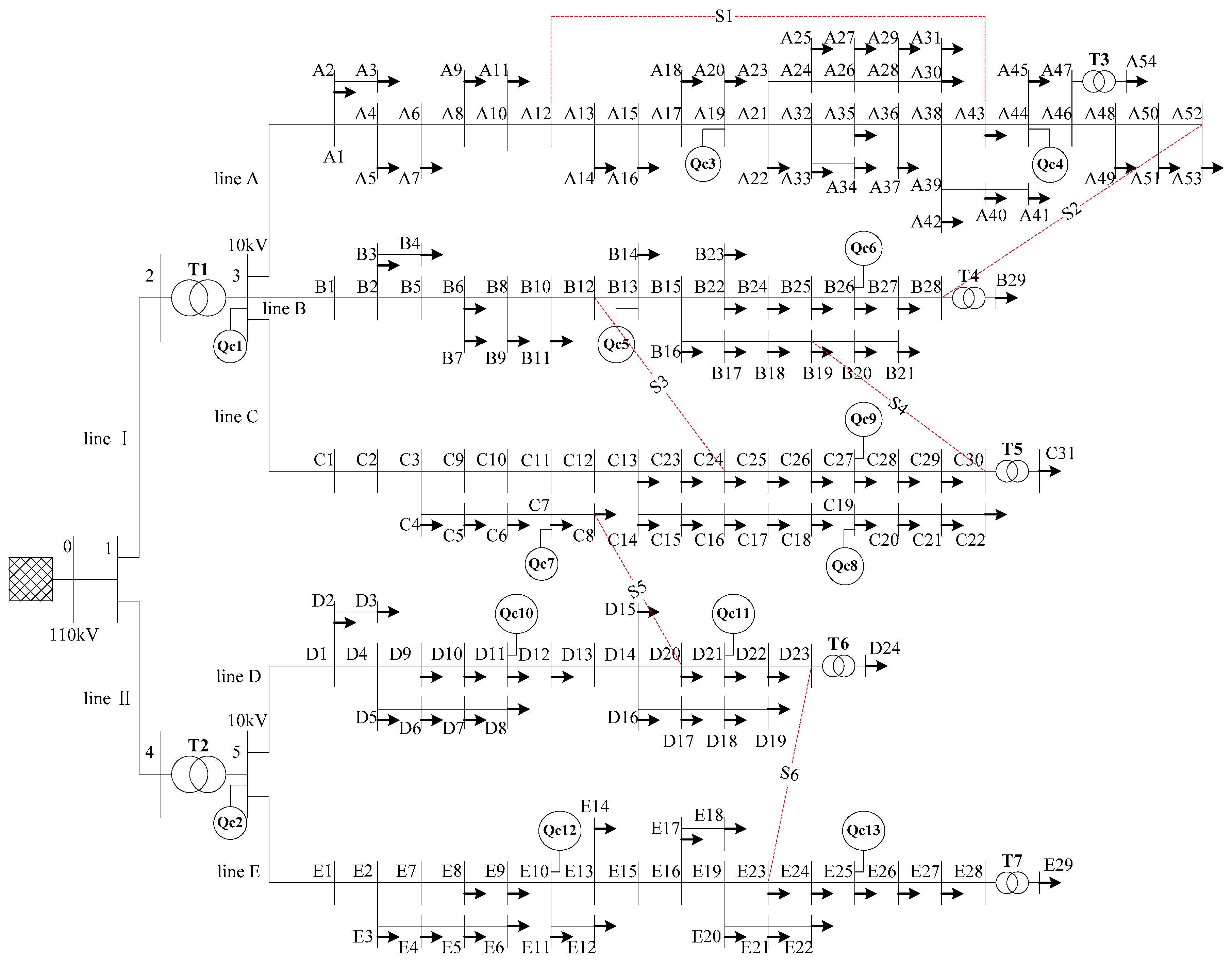
4.1. A Practical Distribution System with 173 Nodes

4.1.1. Case Descriptions of the 173 Nodes System

To demonstrate the effectiveness, the proposed method EWOSM was tested on a practical distribution system with 173 nodes. The head of the system is slack bus, and it is in the low voltage side of a step-down substation from 220 kV to 110 kV. There are two lines of 110 kV connected from the slack bus to two step-down substations from 110 kV to 10 kV respectively, and the substations are connected by five medium-voltage lines of 10 kV, which are named by line A, line B, line C, line D and line E. The single-line diagram of the tested system is shown in Figure 5.
In Figure 5, T1 and T2 are the main transformers in the substation, and the models are both SFZ11-12500/110 with the tap ranging from 0.9 p.u. to 1.1 p.u. by 17 steps. The load is connected to the medium-voltage distribution network by distribution transformer; take T3–T7 for example, the models are S11-400/10, S11-630/10, S11-630/10, S11-630/10 and S11-800/10 respectively, and the taps are fixed to 1.0 p.u. There are thirteen nodes installed by shunt capacitors in the system, where Qc1 and Qc2 are the centralized compensations in the low-voltage side of substation, and Qc3–Qc13 are the feeder compensations. The capacity of capacitors is equal grouped and each group is 50 kvar. The configuration information of capacitors is listed in Table 1. The proposed method EWOSM was coded in MATLAB R2009a (MathWorks, Natick, MA, USA) and run on an Intel i5-3230M 2.6 GHz notebook with 4 GB RAM (Dell, Round Rock, TX, USA).
The historical load data in the test system is from the actual historical database from year 2011 to 2015, and the corresponding reactive power control schemes are also read from the historical database. The missing part of control schemes are calculated by Sequential Quadratic Programming (SQP) based on literature [36], and then the historical database is completed.
In Figure 5, the tie lines are represented by the red dashed lines, and S1–S6 are the tie switches on the corresponding tie lines. The network topology changes through the cooperation of the section switches and tie switches.

4.1.2. The Typical Scenarios Partitioning of the 173 Nodes System

There are eight typical topology scenarios in the historical database from year 2011 to 2015, and the sum of the duration accounts for 94.85% of the total running time of the system. The rest time is accounted for other topology scenarios. The specific information of the typical topology scenarios are shown in Table 2.
According to the information of seasons, weekdays and weekends, there are eight typical load scenarios, and the specific scenario information is shown in Table 3.
The total load forecast curve of one day is shown in Figure 6, and three different load levels are selected out for reactive power optimization calculations, respectively at 2 o’clock, 10 o’clock and 17 o’clock.
Take the high load level (at 17 o’clock) for example to illustrate the calculation processes. Firstly, it is determined that the topology at the time belongs to the first type of the typical topology scenarios according to Table 2, and the typical scenario lasts for 10,512 h from year 2011 to 2015, which can be converted to 438 days. Besides, the day belongs to the typical summer weekdays according to the date, and the typical load scenario lasts for 328 days from year 2011 to 2015. Take the intersection of the two typical scenarios, and there are 217 days in the database that the topology scenario and load scenario are both belonged to the same typical scenario with time to be optimized.

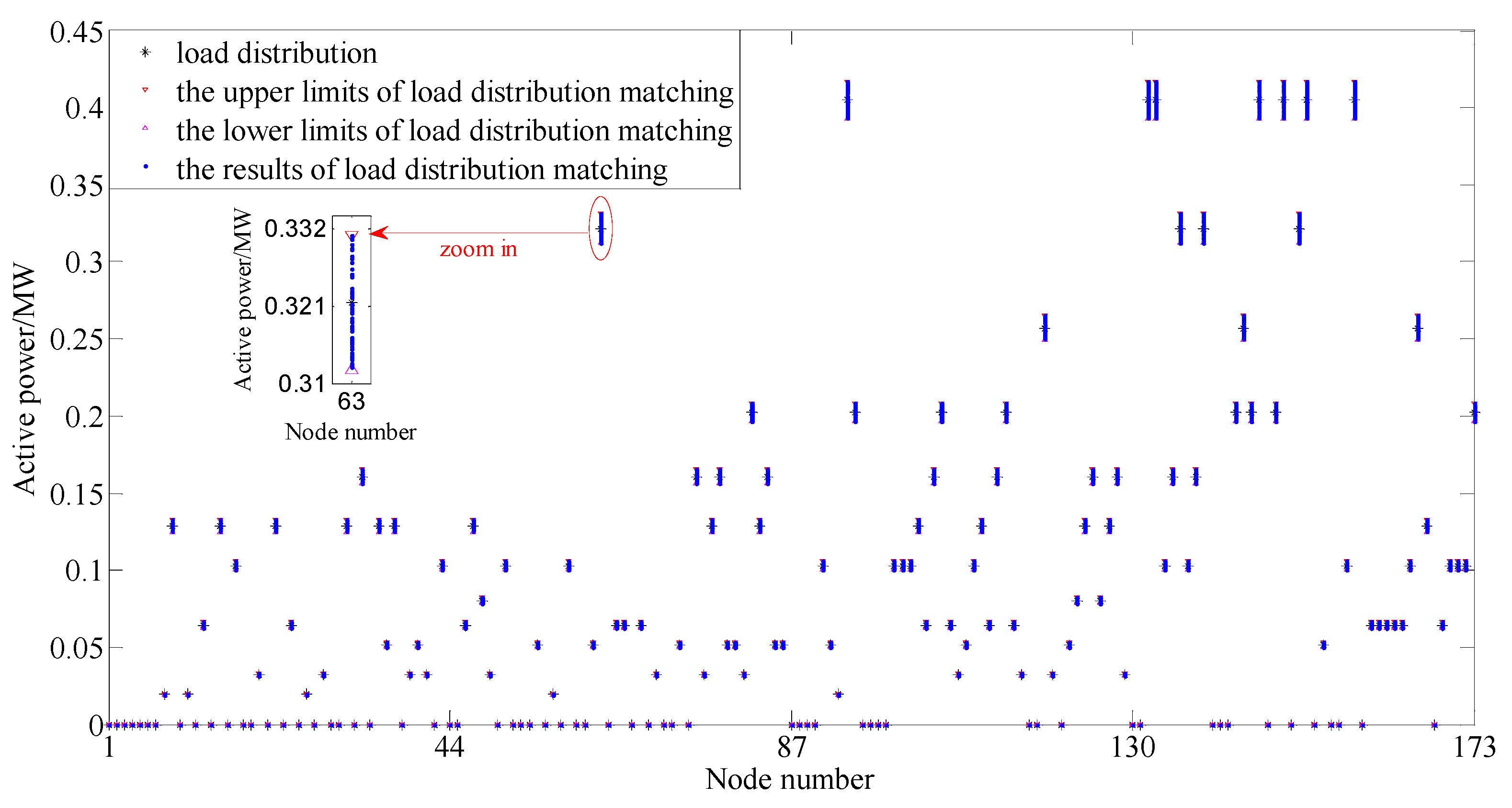
4.1.3. The Load Distribution Matching of the 173 Nodes System

Then, the load distributions at 17 o’clock of the 217 days are matched with the proposed load distribution matching method, and σ is set to the 1% of the load on corresponding nodes. Finally, there are 59 alternatives are selected out, and the results of load distribution matching are shown in Figure 7.
As shown in Figure 7, the black symbols * represent the load distribution at 17 o’clock; the red symbols ˅ and magenta symbols ˄ respectively indicate the upper and lower limits of the load distribution matching, that is, the 1% positive and negative deviation of the load on each node at 17 o’clock; the blue points represent the 59 load distributions from the matching results. It can be seen obviously from the partial enlarged diagram at the top-left corner of Figure 7 that the matched 59 load distributions are all within the 1% positive and negative deviation of the load on each node at 17 o’clock.

4.1.4. The Entropy Weight Method of the 173 Nodes System

Power flow is calculated in turn with the 59 alternatives based on the load at 17 o’clock, and the corresponding network loss, node voltage offset and minimum module-eigenvalue are shown in Figure 8, which are calculated according to Equations (2)–(4).
As shown in Figure 8, there are some cases that the network loss or node voltage offset of the 59 alternatives is similar or the same. It is because that a part of the control schemes of the alternatives may be same or similar. The weights of the network loss, node voltage offset and minimum module-eigenvalue are 0.5402, 0.2106 and 0.2492 respectively, and the optimal scheme is the thirty-second alternative. The specific optimal scheme and results are shown in Table 4.

4.1.5. Results, Comparisons and Analysis of the 173 Nodes System

The proposed method EWOSM is compared with conventional reactive power optimization method to verify the validity and effectiveness. Genetic Algorithm (GA) and SQP method are chosen as the representatives of the existing artificial intelligence algorithms and traditional mathematical methods respectively to compare with EWOSM. The optimal results of the three methods under three different load levels are shown in Table 4. GA method based on literature [37,38] is used as the solution of conventional reactive power optimization, and the specific parameters are as follows: crossover rate is 0.8, mutation rate is 0.2, population size is 20, the maximum number of iterations is 100, and the algorithm will stop with no evolution for more than 50 continuous generations. And SQP method is based on literature [36].
It can be seen from Table 4 that the differences of network loss of GA, SQP and EWOSM under the three different load levels are less than 1%, and the differences of minimum module-eigenvalue are less than 1.5%, which proves the validity and effectiveness of the proposed EWOSM. Besides, the three methods are also applied to several different scales of test systems, including the standard distribution system of IEEE 33 nodes [39], PG & E 69 nodes [40] and a practical distribution system with 292 nodes, and the results are listed in Appendix A (Table A1) due to length of the article, which can further proof the effectiveness of EWOSM.

4.2. The Influence of System Scale and the Number of Control Variables on the Computation Time

In order to verify the superiority of the proposed method in terms of computing speed, several test systems are simulated respectively to analyze the influence of the system scale and the number of control variables on the computation time, based on the historical data from year 2011 to 2015. To fully verify the impact of the two factors on the computation time, the network topologies of the following test systems are assumed to remain unchanged.

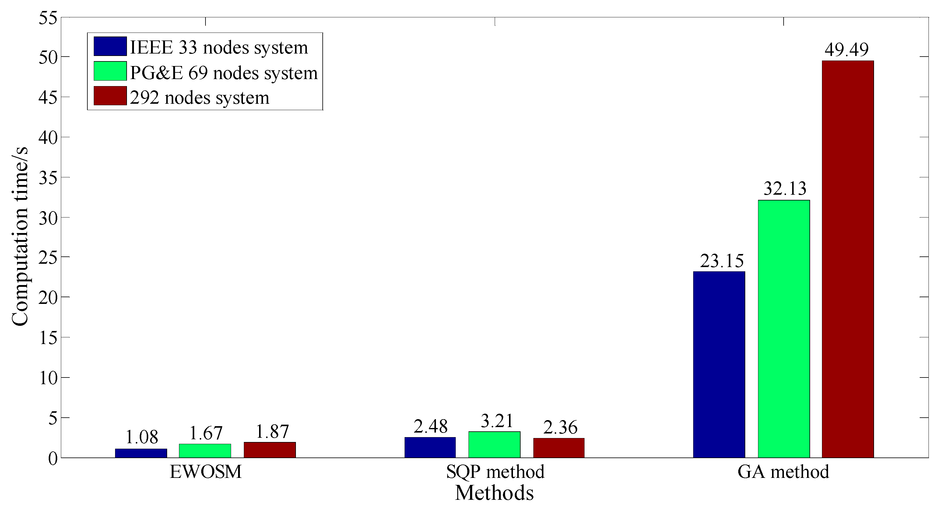
4.2.1. Analysis of the Influence of System Scale on the Computation Time

Firstly, test the impact of the system scale on the computation time with three systems, containing the standard distribution system of IEEE 33 nodes, PG & E 69 nodes and a practical 292 distribution system with 292 nodes. The three testing systems all contain one on-load tap changer (OLTC) and three shunt capacitor compensation nodes, and the specific configuration information of capacitors are shown in Table 5. The single group capacity of capacitors is 50 kvar, and tap of OLTC is 1 ± 8 × 1.25%.
The proposed EWOSM, GA method and SQP method are used for reactive power optimization respectively on the three testing systems, and the comparison of computation time is shown in Figure 9.
As shown in Figure 9 that while the number of control variables is the same, the computation time of EWOSM and GA method increases with the increasing of the system scale, but the computation time of SQP method has little relevance to the system scale. The reason is that power load of all nodes need to be matched in the load distribution matching. Therefore, the computation time of EWOSM is positive correlated to the number of system nodes, but it is still much shorter than GA method.

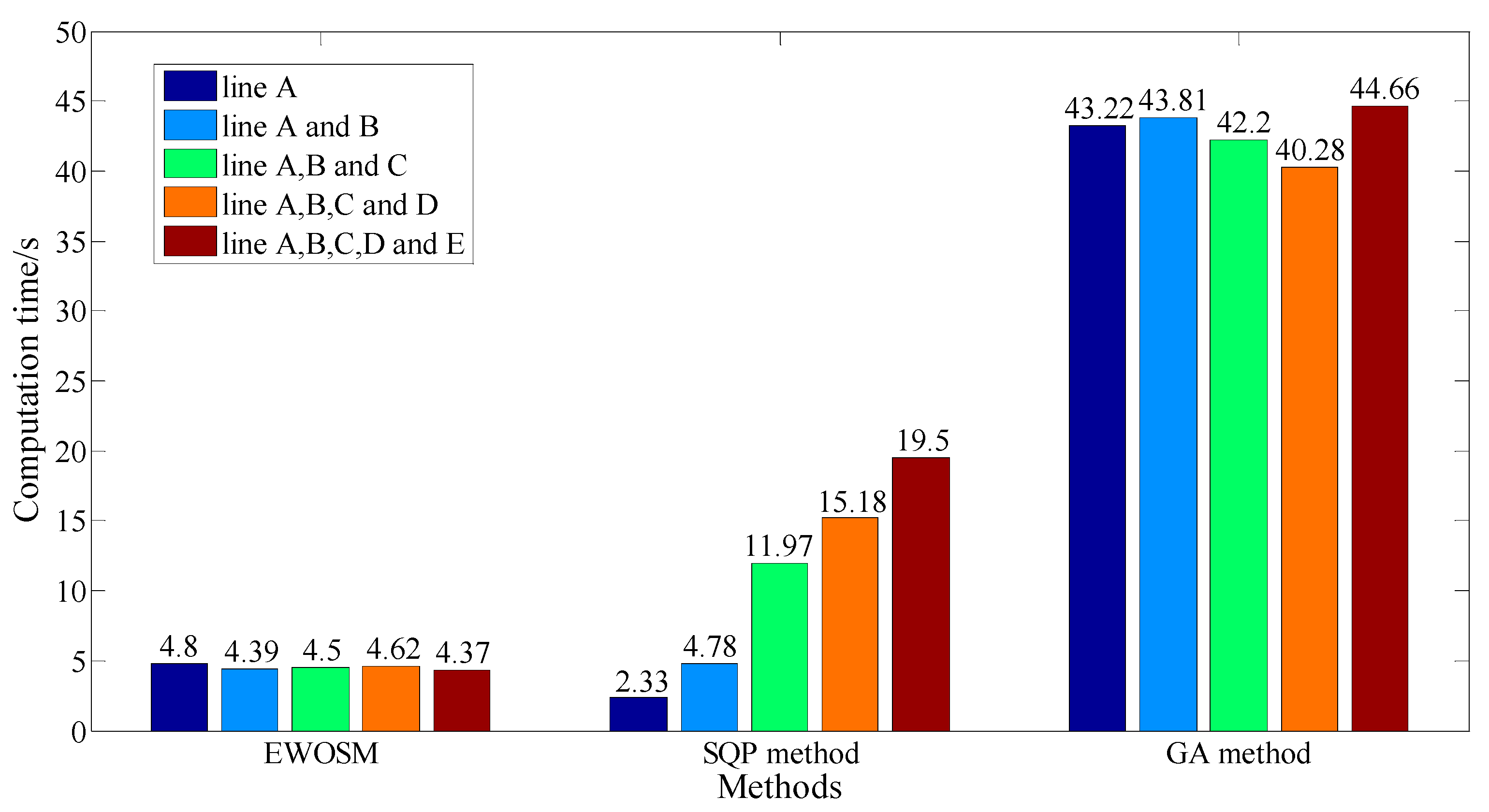
4.2.2. Analysis of the Influence of the Number of Control Variables on the Computation Time

Next, the influence of the number of control variables on computation time is tested on the 173 nodes system mentioned in Section 4.1. The system contains five medium-voltage lines of 10 kV and fifteen control variables. Adjust the number of lines that take part in reactive power optimization, and then the number of control variables changes correspondingly. The proposed EWOSM, GA method and SQP method are used to calculate the optimal results respectively. The specific setting of control variables is shown in Table 6 and the comparison of computation time is shown in Figure 10.
It can be seen from Figure 10 that the computation time of SQP method increases with the increasing of the number of control variables, while the computation time of EWOSM and GA method are less affected by the number of control variables. While the number of control variables is small, the advantage in computation time of the method proposed is not obvious compared with the existing methods. But with the increasing of the number of control variables, the advantage is obviously enhanced.

4.3. The Combination of EWOSM and SQP Method

As the proposed method EWOSM is based on the analysis and comparison of large amount of historical data, in practical applications, some historical data may be missing and some historical control schemes are not optimized, which will lead to that the result of EWOSM is more like a suboptimal feasible solution rather than a global solution. In practical scenarios that the global optimal solution is necessary, EWOSM can be used in combination with GA method, neighborhood search method, SQP method and other existing methods to speed up the convergence and ensure the global optimization.
In this case, comparison of objective function values, computation time and convergence algebra of three different methods is designed to prove the effectiveness of the proposed hybrid method, in which the result of EWOSM is treated as an initial solution of SQP method. The computation time and results of EWOSM, the hybrid method and SQP method are shown in Table 7.
It can be seen from Table 7 that the objective function of the three methods is almost the same, which proves the validity of the hybrid method proposed. From the view of computation time, the time of hybrid method is 7.41 s, which is reduced by 62% than SQP method. Besides, from the view of convergent rate, the hybrid method converges in the ninth iteration, which is much less than the forty-second iteration of SQP method. The comparison result illustrates that the effect of the proposed hybrid method in speeding up the convergence and reducing the computation time is remarkable.

5. Conclusions

A reactive power optimization method in distribution network based on EWOSM is presented. The proposed method is tested on several systems with different scales and comparison has been made with GA method and SQP method. The results have proved the validity and effectiveness of the proposed method EWOSM. The contributions and the novelties can be concluded as follows:
(1)
The proposed EWOSM can rapidly and accurately select out the optimal scheme from large amount of historical data. And the advantage in computation time is remarkable than existing methods.
(2)
The proposed EWOSM can be used in combination with existing methods to speed up the convergence and ensure the global optimization.
(3)
As the proposed EWOSM is based on the analysis of large amount of historical data, it is more suitable for the distribution system that has relatively stable load and complete historical database; otherwise the proposed EWOSM needs to cooperate with existing methods. The application of big data theory and method in reactive power optimization needs to be further improved and perfected.

Acknowledgments

This work was supported by Science and Technology Project of State Grid Corporation of China (EPRIPDKJ (2015) 1495), and Beijing Natural Science Foundation (3172039).

Author Contributions

Yuqi Ji and Guangfei Geng conceived, designed and performed the experiments; Yuqi Ji, Keyan Liu, Dongli Jia and Kaiyuan He analyzed the data; Wanxing Sheng and Xiaoli Meng contributed the power load data and provided some suggestions on the experiments and manuscript; Yuqi Ji, Keyan Liu and Guangfei Geng wrote the paper.

Conflicts of Interest

The authors declare no conflict of interest.

Appendix A. The Calculation Results of Three Methods with Different Scales of Systems

Table A1. The calculation results of three methods in different scales of systems.
IEEE 33 Nodes SystemPG&E 69 Nodes System292 Nodes System
EWOSMGASQPEWOSMGASQPEWOSMGASQP
Optimal schemeC1/kvar300300300300300300750750750
C2/kvar400400400100010501050300300300
C3/kvar800800800200200200400400400
T1 + 4 × 1.25%1 + 4 × 1.25%1 + 4 × 1.25%
Network loss/kW75.575.575.5124.8124.7124.793.893.893.8
Node voltage offset1.271.271.274.494.504.508.698.698.69
Minimum module-eigenvalue0.01690.01690.01690.009910.009920.009920.001550.001550.00155
Computation time/s1.0823.152.481.6732.133.211.8749.492.36

References

  1. Zhang, B.; Hou, P.; Hu, W.; Soltani, M.; Chen, C.; Chen, Z. A reactive power dispatch strategy with loss minimization for a DFIG-based wind farm. IEEE Trans. Sustain. Energy 2016, 7, 914–923. [Google Scholar] [CrossRef]
  2. Chavez, D.; Espinosa, S.; Cazco, D.A. Reactive power optimization of the electric system based on minimization of losses. IEEE Trans. Smart Grid 2016, 14, 4540–4546. [Google Scholar] [CrossRef]
  3. Xue, Y.; Zhang, X.P. Reactive power and AC voltage control of LCC HVDC system with controllable capacitors. IEEE Trans. Power Syst. 2017, 32, 753–764. [Google Scholar] [CrossRef]
  4. Garcia, A.M.; Mastromauro, R.A.; Sanchez, T.G.; Pugliese, S.; Liserre, M.; Stasi, S. Reactive power flow control for PV inverters voltage support in LV distribution networks. IEEE Trans. Smart Grid 2017, 8, 447–456. [Google Scholar] [CrossRef]
  5. Nie, Y.; Du, Z.; Li, J. AC–DC optimal reactive power flow model via predictor–corrector primal-dual interior-point method. IET Gener. Transm. Distrib. 2013, 7, 382–390. [Google Scholar] [CrossRef]
  6. Abril, I.P.; Quintero, J.A.G. VAr compensation by sequential quadratic programming. IEEE Trans. Power Syst. 2003, 18, 36–41. [Google Scholar] [CrossRef]
  7. Zhang, C.; Chen, H.; Ngan, H. Reactive power optimisation considering wind farms based on an optimal scenario method. IET Gener. Transm. Distrib. 2016, 10, 3736–3744. [Google Scholar] [CrossRef]
  8. Chen, S.; Hu, W.; Chen, Z. Comprehensive cost minimization in distribution networks using segmented-time feeder reconfiguration and reactive power control of distributed generators. IEEE Trans. Power Syst. 2016, 31, 983–993. [Google Scholar] [CrossRef]
  9. Chen, F.; Chen, M.; Li, Q.; Meng, K.; Guerrero, J.M.; Abbott, D. Multiagent-based reactive power sharing and control model for islanded microgrids. IEEE Trans. Sustain. Energy 2016, 7, 1232–1244. [Google Scholar] [CrossRef]
  10. Cimino, M.; Pagilla, P.R. Reactive power control for multiple synchronous generators connected in parallel. IEEE Trans. Power Syst. 2016, 31, 4371–4378. [Google Scholar] [CrossRef]
  11. Lin, C.; Wu, W.; Zhang, B.; Wang, B.; Zheng, W.; Li, Z. Decentralized reactive power optimization method for transmission and distribution networks accommodating large-scale DG integration. IEEE Trans. Sustain. Energy 2017, 8, 363–373. [Google Scholar] [CrossRef]
  12. Ding, T.; Liu, S.; Wu, Z.; Bie, Z. Sensitivity-based relaxation and decomposition method to dynamic reactive power optimisation considering DGs in active distribution networks. IET Gener. Transm. Distrib. 2017, 11, 37–48. [Google Scholar] [CrossRef]
  13. Salih, S.N.; Chen, P. On coordinated control of OLTC and reactive power compensation for voltage regulation in distribution systems with wind power. IEEE Trans. Power Syst. 2016, 31, 4026–4035. [Google Scholar] [CrossRef]
  14. Sheng, W.; Liu, K.Y.; Liu, Y.; Ye, X.; He, K. Reactive power coordinated optimisation method with renewable distributed generation based on improved harmony search. IET Gener. Transm. Distrib. 2016, 10, 3152–3162. [Google Scholar] [CrossRef]
  15. Ugranli, F.; Karatepe, E.; Nielsen, A.H. MILP approach for bilevel transmission and reactive power planning considering wind curtailment. IEEE Trans. Power Syst. 2017, 32, 652–661. [Google Scholar] [CrossRef]
  16. Edrah, M.; Lo, K.L.; Anaya-Lara, O. Reactive power control of DFIG wind turbines for power oscillation damping under a wide range of operating conditions. IET Gener. Transm. Distrib. 2016, 10, 3777–3785. [Google Scholar] [CrossRef]
  17. Robbins, B.A.; Domínguez-García, A.D. Optimal reactive power dispatch for voltage regulation in unbalanced distribution systems. IEEE Trans. Power Syst. 2016, 31, 2903–2913. [Google Scholar] [CrossRef]
  18. Yang, F.; Li, Z. Improve distribution system energy efficiency with coordinated reactive power control. IEEE Trans. Power Syst. 2016, 31, 2518–2525. [Google Scholar] [CrossRef]
  19. Macedo, L.H.; Montes, C.V.; Franco, J.F.; Rider, M.J.; Romero, R. MILP branch flow model for concurrent AC multistage transmission expansion and reactive power planning with security constraints. IET Gener. Transm. Distrib. 2016, 10, 3023–3032. [Google Scholar] [CrossRef]
  20. Wu, X.; Zhu, X.; Wu, G.Q.; Ding, W. Data mining with big data. IEEE Trans. Knowl. Data Eng. 2014, 26, 97–107. [Google Scholar]
  21. Hu, H.; Wen, Y.; Chua, T.S.; Li, X. Toward scalable systems for big data analytics: A technology tutorial. IEEE Access 2014, 2, 652–687. [Google Scholar]
  22. Mao, B.; Jiang, H.; Wu, S.; Tian, L. Leveraging data deduplication to improve the performance of primary storage systems in the cloud. IEEE Trans. Comput. 2016, 65, 1775–1788. [Google Scholar] [CrossRef]
  23. Cherubini, G.; Jelitto, J.; Venkatesan, V. Cognitive storage for big data. Computer 2016, 49, 43–51. [Google Scholar] [CrossRef]
  24. Wang, B.; Fang, B.; Wang, Y.; Liu, H.; Liu, Y. Power system transient stability assessment based on big data and the core vector machine. IEEE Trans. Smart Grid 2016, 7, 2561–2570. [Google Scholar] [CrossRef]
  25. Peppanen, J.; Reno, M.J.; Broderick, R.J.; Grijalva, S. Distribution system model calibration with big data from AMI and PV inverters. IEEE Trans. Smart Grid 2016, 7, 2497–2506. [Google Scholar] [CrossRef]
  26. Zhu, J.; Zhuang, E.; Fu, J.; Baranowski, J.; Ford, A.; Shen, J. A framework-based approach to utility big data analytics. IEEE Trans. Power Syst. 2016, 31, 2455–2462. [Google Scholar] [CrossRef]
  27. Shaker, H.; Zareipour, H.; Wood, D. A data-driven approach for estimating the power generation of invisible solar sites. IEEE Trans. Smart Grid 2016, 7, 2466–2476. [Google Scholar] [CrossRef]
  28. Vaccaro, A.; Cañizares, C.A. An affine arithmetic-based framework for uncertain power flow and optimal power flow studies. IEEE Trans. Power Syst. 2017, 32, 274–288. [Google Scholar] [CrossRef]
  29. Pan, S.; Morris, T.; Adhikari, U. Developing a hybrid intrusion detection system using data mining for power systems. IEEE Trans. Smart Grid 2015, 6, 3104–3113. [Google Scholar] [CrossRef]
  30. Williams, T.; Crawford, C. Probabilistic load flow modeling comparing maximum entropy and gram-charlier probability density function reconstructions. IEEE Trans. Power Syst. 2013, 28, 272–280. [Google Scholar] [CrossRef]
  31. Samui, A.; Samantaray, S.R. Wavelet singular entropy-based islanding detection in distributed generation. IEEE Trans. Power Deliv. 2013, 28, 411–418. [Google Scholar] [CrossRef]
  32. Zhang, J.F.; Tse, C.T.; Wang, W.; Chung, C.Y. Voltage stability analysis based on probabilistic power flow and maximum entropy. IET Gener. Transm. Distrib. 2010, 4, 530–537. [Google Scholar] [CrossRef]
  33. Fu, J.; Fan, W.; Li, J.; Zhou, T.; Liu, B.; Chen, R. Study on information fusion method of distribution equipment condition comprehensive evaluation. In Proceedings of the China International Conference on Electricity Distribution, Xi’an, China, 10–13 August 2016. [Google Scholar]
  34. Diao, Y.; Sheng, W.; Liu, K.Y.; He, K.; Meng, X. Research on online cleaning and repair methods of large-scale distribution network load data. Power Syst. Technol. 2015, 3134–3140. [Google Scholar]
  35. Wang, M.; Wu, T. Load restoration optimization based on entropy weight method. In Proceedings of the International Conference on Power and Renewable Energy, Shanghai, China, 21–23 October 2016; IEEE: Piscataway, NJ, USA, 2016; pp. 368–372. [Google Scholar]
  36. Sheng, W.; Liu, K.Y.; Cheng, S.; Meng, X.; Dai, W. A trust region SQP method for coordinated voltage control in smart distribution grid. IEEE Trans. Smart Grid 2015, 7, 381–391. [Google Scholar] [CrossRef]
  37. Gong, C.; Wang, Z. Proficient in MATLAB Optimization Calculation, 2nd ed.; Publishing House of Electronics Industry: Beijing, China, 2012; pp. 314–318. [Google Scholar]
  38. Iba, K. Reactive power optimization by genetic algorithm. IEEE Trans. Power Syst. 1994, 9, 685–692. [Google Scholar]
  39. Baran, M.E.; Wu, F.F. Network reconfiguration in distribution systems for loss reduction and load balancing. IEEE Trans. Power Deliv. 1989, 4, 1401–1407. [Google Scholar] [CrossRef]
  40. Baran, M.E.; Wu, F.F. Optimal capacitor placement on radial distribution systems. IEEE Trans. Power Deliv. 1989, 4, 725–734. [Google Scholar] [CrossRef]
Figure 1. The typical daily load curves of different scenarios in a certain region: (a) weekdays in four seasons; and (b) weekends in four seasons.
Applsci 07 00787 g001
Figure 2. Schematic diagram of load distribution matching.
Applsci 07 00787 g002
Figure 3. Flow chart of load distribution matching.
Applsci 07 00787 g003
Figure 4. Flow chart of reactive power optimization in distribution network based on entropy-weight method.
Applsci 07 00787 g004
Figure 5. Connection diagram of a practical distribution network with 173 nodes.
Applsci 07 00787 g005
Figure 6. The load curve of the next day.
Applsci 07 00787 g006
Figure 7. The result of load distribution matching at 17:00.
Applsci 07 00787 g007
Figure 8. The evaluation indexes of alternatives: (a) the network loss; and (b) the node voltage offset; (c) the minimum module-eigenvalue.
Applsci 07 00787 g008
Figure 9. The comparison of computation time with three methods in different scale distribution networks.
Applsci 07 00787 g009
Figure 10. The comparison of computation time with three methods under different number of control variables.
Applsci 07 00787 g010
Table 1. The configuration of capacitors in 173 nodes system.
Capacitors NameConnected Bus NumberCompensation Capacity/KvarCapacitors NameConnected Bus NumberCompensation Capacity/Kvar
Qc132000Qc8C19600
Qc252000Qc9C271200
Qc3A191200Qc10D112000
Qc4A441000Qc11D211200
Qc5B131200Qc12E102000
Qc6B26800Qc13E25800
Qc7C7600
Table 2. The typical topology scenarios information of the 173 nodes system.
No.The State of Tie SwitchesThe Disconnected FeedersScenario Duration/hThe Ratio of Duration
S1S2S3S4S5S6
Typical topology Scenario 1OpenOpenOpenOpenOpenOpen/10,51223.99%
Typical topology Scenario 2CloseOpenCloseOpenCloseOpenA12–A13, C23–C24, D14–D20974422.23%
Typical topology Scenario 3CloseCloseOpenOpenOpenCloseA12–A13, A43–A44, E19–E23753617.20%
Typical topology Scenario 4OpenCloseCloseOpenCloseOpenA43–A44, C23–C24, D14–D20657615.01%
Typical topology Scenario 5CloseCloseOpenCloseOpenOpenA12–A13, A43–A44, B18–B1922805.20%
Typical topology Scenario 6OpenCloseCloseCloseCloseOpenA43–A44, B18–B19,
C23–C24, D14–D20
17524.00%
Typical topology Scenario 7CloseOpenCloseCloseOpenCloseA12–A13, B18–B19,
C23–C24, E19–E23
16083.67%
Typical topology Scenario 8CloseCloseCloseOpenCloseOpenA12–A13, A43–A44,
C23–C24, D14–D20
15603.56%
Sum/// //41,56894.85%
Table 3. The typical load scenarios information of the 173 nodes system.
No.The Typical Load ScenariosThe Number of DaysNo.The Typical Load ScenariosThe Number of Days
1Weekday in Spring3285Weekday in Autumn325
2Weekend in Spring1326Weekend in Autumn130
3Weekday in Summer3287Weekday in Winter323
4Weekend in Summer1328Weekend in Winter128
Table 4. The results of reactive power optimization with two methods under different load levels.
High Load Level (at 17 o’clock)Middle Load Level (at 10 o’clock)Low Load Level (at 2 o’clock)
GASQPEWOSMGASQPEWOSMGASQPEWOSM
Optimal schemesQc1/kvar9504004001000300350950250200
Qc2/kvar1000800850900550550950350350
Qc3/kvar600800850800700650450550500
Qc4/kvar900550550450450400500350300
Qc5/kvar105095010001150800800600600600
Qc6/kvar600450450250400350350300300
Qc7/kvar600500500450400400300300300
Qc8/kvar500500500450450450350350300
Qc9/kvar1200800800700650600450500500
Qc10/kvar1900115012001150950950650700700
Qc11/kvar65011501150850950900850700700
Qc12/kvar19001550165014501350130090010501000
Qc13/kvar800750800550650650450500450
T11 + 6 × 1.25%1 + 6 × 1.25%1 + 6 × 1.25%
T21 + 6 × 1.25%1 + 6 × 1.25%1 + 6 × 1.25%
Network loss/kW637.16632.86631.40494.76494.34495.39342.93342.11342.40
Node voltage offset32.2816.82618.4029.8419.57817.8433.0925.33223.15
Minimum module-eigenvalue0.005790.005680.005690.005900.005820.005810.006060.006010.00599
Computation time/s44.66313.644.3744.2910.1434.84639.211.4973.925
Table 5. The configuration of capacitors in three different scale distribution networks.
No.IEEE 33 Nodes SystemPG&E 69 Nodes System292 Nodes System
Connected BusCapacity/KvarConnected BusCapacity/KvarConnected BusCapacity/Kvar
Capacitors C11350035500291200
Capacitors C223500451200157600
Capacitors C329100061500277500
Table 6. The comparison of computation time with three methods varied with the number of control variables.
The Line Participation in Reactive Power ControlThe Number of Control VariablesThe Specific Control Variables
Line A6T1, T2, Qc1–Qc4
Line A and B8T1, T2, Qc1–Qc6
Line A, B and C11T1, T2, Qc1–Qc9
Line A, B, C and D13T1, T2, Qc1–Qc11
Line A, B, C, D and E15T1, T2, Qc1–Qc13
Table 7. Comparison of computation time and results with three methods.
MethodEWOSMThe Hybrid MethodSQP Method
Network loss/kW631.40632.02632.75
Node voltage offset18.4017.1816.71
Minimum module-eigenvalue0.005690.005680.00567
Convergence algebra/942
Computation time/s4.377.4119.50

