
Data Mining Approaches for Landslide Susceptibility Mapping in Umyeonsan, Seoul, South Korea


1
Department of Geoinformatics, University of Seoul, 163 Seoulsiripdaero, Dongdaemun-gu, Seoul 02504, Korea
2
Center for Environmental Assessment Monitoring, Environmental Assessment Group, Korea Environment Institute (KEI), Sejong-si 30147, Korea
*
Authors to whom correspondence should be addressed.
Appl. Sci. 2017, 7(7), 683; https://doi.org/10.3390/app7070683
Submission received: 8 June 2017
/
Revised: 26 June 2017
/
Accepted: 27 June 2017
/
Published: 2 July 2017
(This article belongs to the Special Issue Application of Artificial Neural Networks in Geoinformatics)
Abstract
:The application of data mining models has become increasingly popular in recent years in assessments of a variety of natural hazards such as landslides and floods. Data mining techniques are useful for understanding the relationships between events and their influencing variables. Because landslides are influenced by a combination of factors including geomorphological and meteorological factors, data mining techniques are helpful in elucidating the mechanisms by which these complex factors affect landslide events. In this study, spatial data mining approaches based on data on landslide locations in the geographic information system environment were investigated. The topographical factors of slope, aspect, curvature, topographic wetness index, stream power index, slope length factor, standardized height, valley depth, and downslope distance gradient were determined using topographical maps. Additional soil and forest variables using information obtained from national soil and forest maps were also investigated. A total of 17 variables affecting the frequency of landslide occurrence were selected to construct a spatial database, and support vector machine (SVM) and artificial neural network (ANN) models were applied to predict landslide susceptibility from the selected factors. In the SVM model, linear, polynomial, radial base function, and sigmoid kernels were applied in sequence; the model yielded 72.41%, 72.83%, 77.17% and 72.79% accuracy, respectively. The ANN model yielded a validity accuracy of 78.41%. The results of this study are useful in guiding effective strategies for the prevention and management of landslides in urban areas.

1. Introduction
The rapid growth in data due to the development of information and communication technology (ICT) has spurred the demand for data mining, which is generally considered to be the most useful analytical tool in the analysis of large data sets. Data mining has been defined in various ways previously, and is commonly referred to as an exploratory analysis tool for large amounts of data [1]. Therefore, data mining is a process of finding useful information that is not easily exposed in a large amount of data, most recently known as “big data”.
With the rapid growth of ICT since the 1980s, countries and corporations have made significant efforts to build databases to store and manage vast amounts of data. Rational and rapid decision-making is necessary to increase the utilization of large-scale databases. In this environment, it has become important to find meaningful new information that can support optimal decision-making. In this process, an efficient methodology for data mining that extracts not only known information from previously established databases but also information that was not previously known has gained popularity. Therefore, the data mining methodology makes it possible to effectively analyze large amounts of data in a database and the relationships between parameters.
In recent years, storms bringing localized heavy rains have been reported worldwide, and precipitation in the mid-latitude regions has increased since the 20th century [2]. In addition, rapid climate change and abnormal climate conditions have led to extreme weather phenomena, which provide the appropriate conditions for the creation of landslides, and the frequency of landslides has increased accordingly [3]. A landslide is the movement of soil down a slope when the stress exceeds the strength of the soil material due to rapid changes in the natural environment such as heavy rains or earthquakes [4]. Landslides are caused by various factors, such as topography, geology, soil characteristics, forest conditions, and climate variables [5,6,7,8]. The main purpose of this study was to generate and validate a landslide susceptibility map using data mining models for Umyeonsan, South Korea. Therefore, data mining techniques should be used appropriately for the analysis of the relationships between landslides and impact factors on landslides in landslide susceptibility analyses. Additionally, given that the data mining models derive their results from the database, the input data represent a key part in the model. Thus, the database should be constructed using reliable data, such as nationally distributed government data. Remote sensing data is one of the main sources to be used to generate the reliable data [9,10,11].
Due to the complex factors influencing landslides, it is important to perform an appropriate assessment of the potential for landslide susceptibility using data mining techniques. A susceptibility analysis based on data on previous damage should be performed to define landslide susceptibility in areas where landslides are anticipated so that the damage can be predicted in advance and appropriate mitigation measurements adopted. Over the past several decades, a number of data mining approaches have been developed for mapping landslide susceptibility [12,13]. The most commonly used methods are soft computing or statistical techniques such as artificial neural network (ANN) models [14,15], fuzzy logic methods [16,17] or logistic regression models [18,19]. Landslides are caused by multiple interactions between various factors, including geometry, geology, soil characteristics, and vegetation conditions [20,21], and are highly dependent on terrain features [22,23].
As geological hazards, landslides can limit the sustainable development of urban areas, causing environmental damage, serious casualties, and loss of property [24,25]. An appropriate assessment of the susceptibility for landslide damage is required to minimize the complex array of losses. In South Korea, according to an analysis of the scale of landslides by the Korea Forest Service (KFS), the average annual area affected by landslides increased markedly from 231 ha in the 1980s, to 349 ha in the 1990s, and 713 ha in 2000 [26]. Typhoons accompanied by intense storms caused by local climatic conditions often cause significant damage; and landslides are concentrated in the rainy season every summer. Because much of South Korea is mountainous, most studies on landslides in the country have focused on mountainous areas [27,28,29]; e.g., in Jangheung [23] or Yongjin [6,30]. Furthermore, due to the frequency of landslides in mountainous areas, most of the studies in Southeast Asia have been performed in non-urban areas [31,32,33]. Assessment of landslide susceptibility in urban areas could provide an important contribution to minimizing additional damage from these natural disasters; it could be also used to planning and multi hazard assessment [34,35,36,37].
Seoul, the capital of South Korea, also has urban areas occupying mountainous land. Unlike landslides that occur in sparsely populated mountainous areas, landslides that occur in mountainous areas in cities result in significant casualties/fatalities and structural damage. For example, landslides in Umyeonsan located in central Seoul in July 2011 caused unprecedented damage to the city. Following the 2011 Umyeonsan landslide, the downtown area, which had previously been considered safe, was no longer regarded as a landslide-safe zone. Various aspects of Korea’s landslide policy have been re-evaluated and are expected to be revised in the near future. Landslides are more dangerous in urban areas than non-urban mountainous areas. Policies have shifted to preventative and resident-oriented initiatives, with a focus on minimizing injuries to citizens and restoration of their properties after landslides. Therefore, it is important to analyze potential landslide hazards in urban areas.
To apply the model for this type of data mining analysis, a spatial database should first be constructed containing information on the area of landslide damage. Because landslides are difficult to access, the collection of field survey data to build a landslide spatial database is costly and time-consuming. An effective alternative is to build a database using aerial photography and geographic information systems (GISs). Landslides leave traces that last for months or years; hence, aerial imagery can be used to extract data on areas damaged by landslides after the event. Using these data, the susceptibility for landslides can be analyzed by data mining modeling techniques.
2. Study Area
Seoul is the largest city in South Korea and is located in the center of the Korean Peninsula. The total urban area covered by Seoul (approximately 605 km2) is less than 1% of the total land area of South Korea. However, Seoul is one of the most heavily populated cities in the world; over 10 million citizens were recorded in 2011. Thus, the city has a dense and complex transportation system. Natural disasters, including landslides, have the potential to cause serious damage in the city [2]. The study area, Umyeonsan, is an urbanized mountain rising 321.6 m above sea level in the southern sub-central area of Seoul (Figure 1). Due to the fact that it is not very high or steep, the mountain is a popular site for Seoul residents and it has a large transient population
Umyeonsan is comprised of a low mountainous area with a slope of approximately 30° near the top of the mountain. The area is mainly comprised of gneissic rock formed by geomorphological movement and weathering. The composition of biotite gneiss, which is prone to weathering and fault formation, increases its susceptibility to landslides. The foliation structure of the gneiss is sparsely generated due to multiple flexures. The main soil type distributed in the study area is brown forest soil formed from the base materials of biotite gneiss and granite gneiss, which are metamorphic rocks, and the soil texture is sandy loam to loam, which has good drainage. Deep soils and high organic content brown forest soil is distributed in some valley areas in the study area, where the soil texture is silt loam in silt and sand. Due to the soil textures present, the Umyeonsan area is prone to severe weathering, causing the unstable condition of outcrops.
The main forest type in Umyeonsan is temperate deciduous broad-leaved forest. Broad-leaved forest, pine forest, poplar forest, and broad-leaved plantation forest are all present in the study area. The principal species in the forests are similar to those in the central Korean Peninsula: Quercus mongolica, Robinia pseudoacacia, Quercus variabilis, oak trees and Asian black birch.
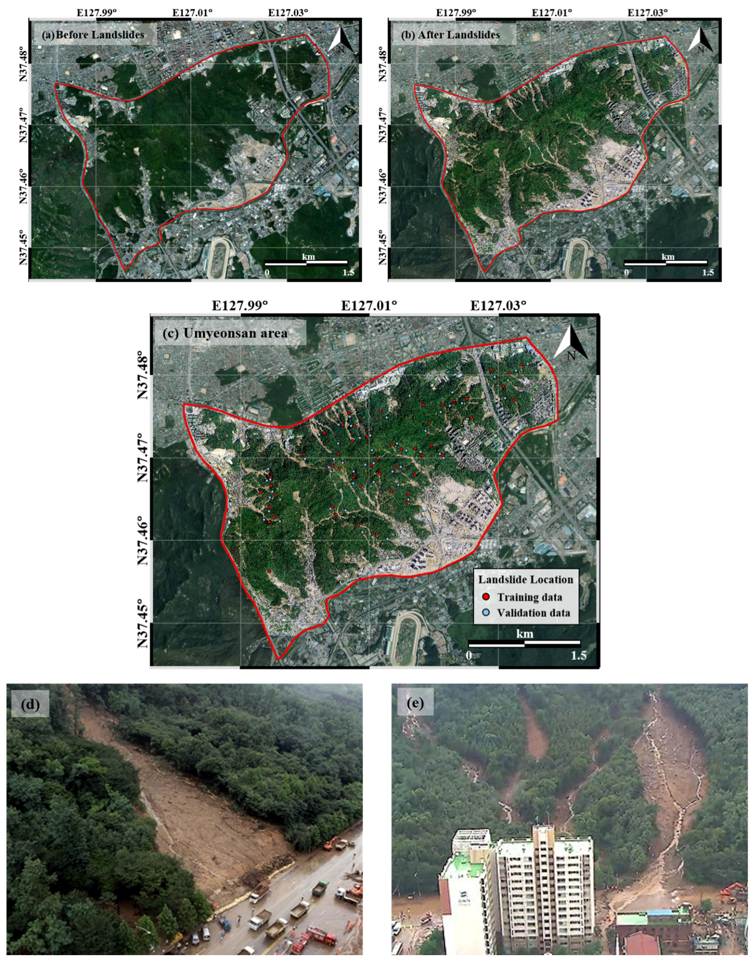
On 27 July 2011, heavy rains occurred in central Korea and a large landslide occurred in Umyeonsan. The heavy rainfall lasted from 26–28 July. The cumulative precipitation in the Seoul metropolitan area was 587.5 mm, which is the largest three-day cumulative precipitation recorded since precipitation monitoring began in Seoul. Based on data from Seocho automatic weather system, the maximum precipitation per hour at the time of the landslide was 85.5 mm [38]. The landslide from the heavy rains affected an area of 73.23 ha. Sixteen people were killed, including 6 residents from the village of Namtaeryeong and 7 residents from the southern area of the southern ring roads; 2 people remained missing, and approximately 400 people were evacuated [39]. The water supply was cut off. Thousands of apartments near Gangnam and Umyeonsan were damaged; and over 20,000 households experienced water problems. Therefore, we chose this landslide to obtain data for our study (Figure 2d,e). The study area was determined by the road and river boundaries in the Umyeonsan area (Figure 2).
3. Data
Given that data mining models are a data-driven methodology, accurate data are essential to build a suitable database. Accurate data on the state of the earth’s surface can be obtained rapidly using aerial photographs, which also effectively capture complicated urban structures. Moreover, despite the high cost of aerial photographs, it is cost-effective to acquire the images of and continuously monitor urban areas due to their dense nature. To acquire accurate data on the landslide occurrence, aerial photographs from before and after the Umyeonsan landslides were used (Figure 2a,b). Location data for the Umyeonsan landslide area were acquired through comparative analysis, as traces of landslides are visible for several years after the events.
In addition, a digital topographic map (1:5000) generated by the National Geographic Information Institute (NGII) was obtained, and geometric correction was performed. Overlay and comparative analysis of the aerial photographs and the 1:5000 digital topographic map indicated the landslide occurrence area (Figure 2c). The mapped landslide occurrence data were finally confirmed by comparison with data surveyed in the field by the Seoul metropolitan government [39].
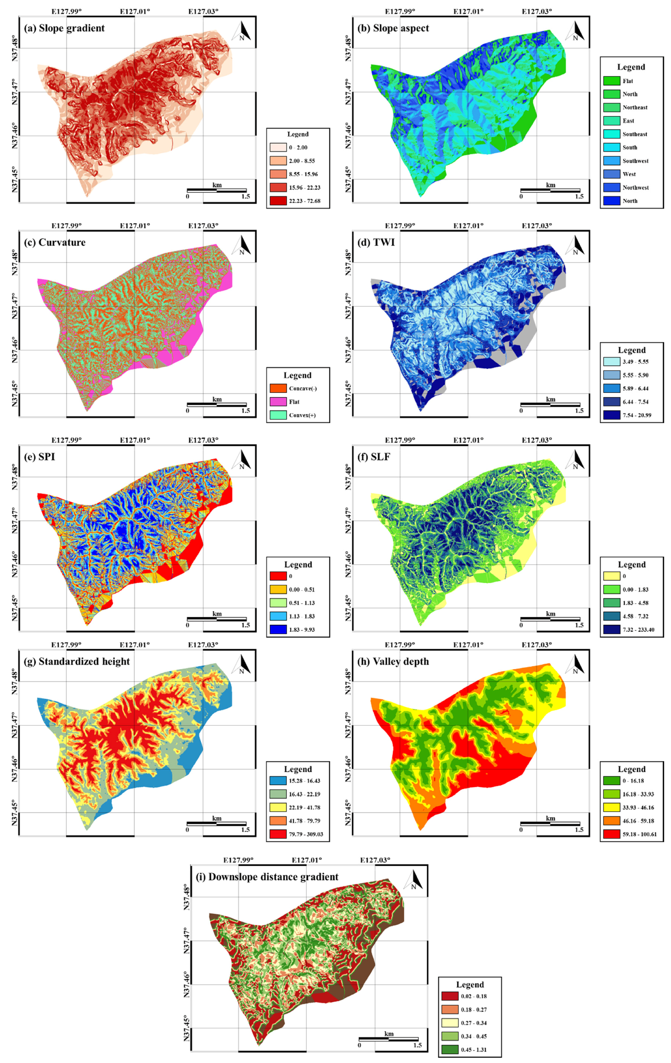
Slopes are established by erosion and sedimentation of terrain surfaces and have a key effect on landslide occurrence as they affect the flow of water and the soil characteristics [42]. Therefore, among the factors influencing landslides, topographic factors were preferentially considered and were used as input data to identify the relationships with landslide occurrence (Figure 3). Prior to calculation of the topographic factors, a triangulated irregular network (TIN) was produced from a pre-generated topographic map, and a digital elevation model (DEM) was created using ArcGIS 10.1 (ESRI, Redlands, LA, USA).
All topographic factors were calculated from the DEM using ArcGIS software (ESRI, Redlands, LA, USA). The slope, indicated as the angle to the horizontal plane or the ratio of the vertical height to the horizontal distance as a percentage, was calculated using the SLOPE tool. The ASPECT tool was used to calculate the aspect, the compass direction of the slope faces. The curvature values of the terrain surface were calculated using the CURVATURE tool. The curvature represents the morphological characteristics of the study area; an upwardly convex surface possesses a positive value, while an upwardly concave surface possesses a negative value.
The topographic wetness index (TWI) is defined for a steady state. The index is commonly used for hydrological processes to quantify the disposition of water flow and the impact on the topography [43]. The TWI is calculated by the run-off model as follows, which reflects the accumulation of water at a specific point in the catchment area and the force of gravity on the water in the area [43].
where α is the cumulative upslope area drained per unit contour length in a cell, and β is the local slope angle of the cell.
The stream power index (SPI) estimates the erosion power of a stream, which affects the stability of the area. Therefore, it is generally used to determine the locations for performing soil conservation measures to reduce the erosive effects of concentrated surface runoff. SPI can be calculated as follows [44]:
where As is the area of the target point of the study area, and β is the slope angle.
After calculating the slope, the slope length factor (SLF) for average erosion is calculated using the Revised Universal Soil Loss Equation (RUSLE) [45]. The SLF for slope of length λ is represented as:
where the constant value 72.6 of the RUSLE is in feet, and the variable, m, is the slope-length exponent calculated from the local slope angle β [45]. The SLF is influenced by the ratio of rill erosion to interrill erosion, β. Rill erosion is caused by flow, while interrill erosion is caused by the effects from rainfall.
System for Automated Geoscientific Analyses (SAGA) GIS were used to calculate additional topographic factors [46]. The standardized height is the absolute height multiplied by the normalized height of the study area; normalized height is the normalization of the height of the study area between 0 and 1. The standardized height was calculated using linear regression to yield the suitable parameters for prediction of the soil attributes by simplifying the complex terrain states [47]. The valley depth is the vertical distance of the specific point from the base level of the channel network [46]. The elevation of the channel network base level is interpolated, and the valley depth is calculated by subtracting the base level of the channel network from the DEM [46]. The downslope distance gradient is a quantitative estimation of the hydraulic gradient. The downslope distance gradient is obtained by calculating the downhill distance when water loses a determined quantity of energy from precipitation [48]. tan identifies the downslope distance gradient:
where d and are the elevation and the horizontal distance to the reference point, respectively.
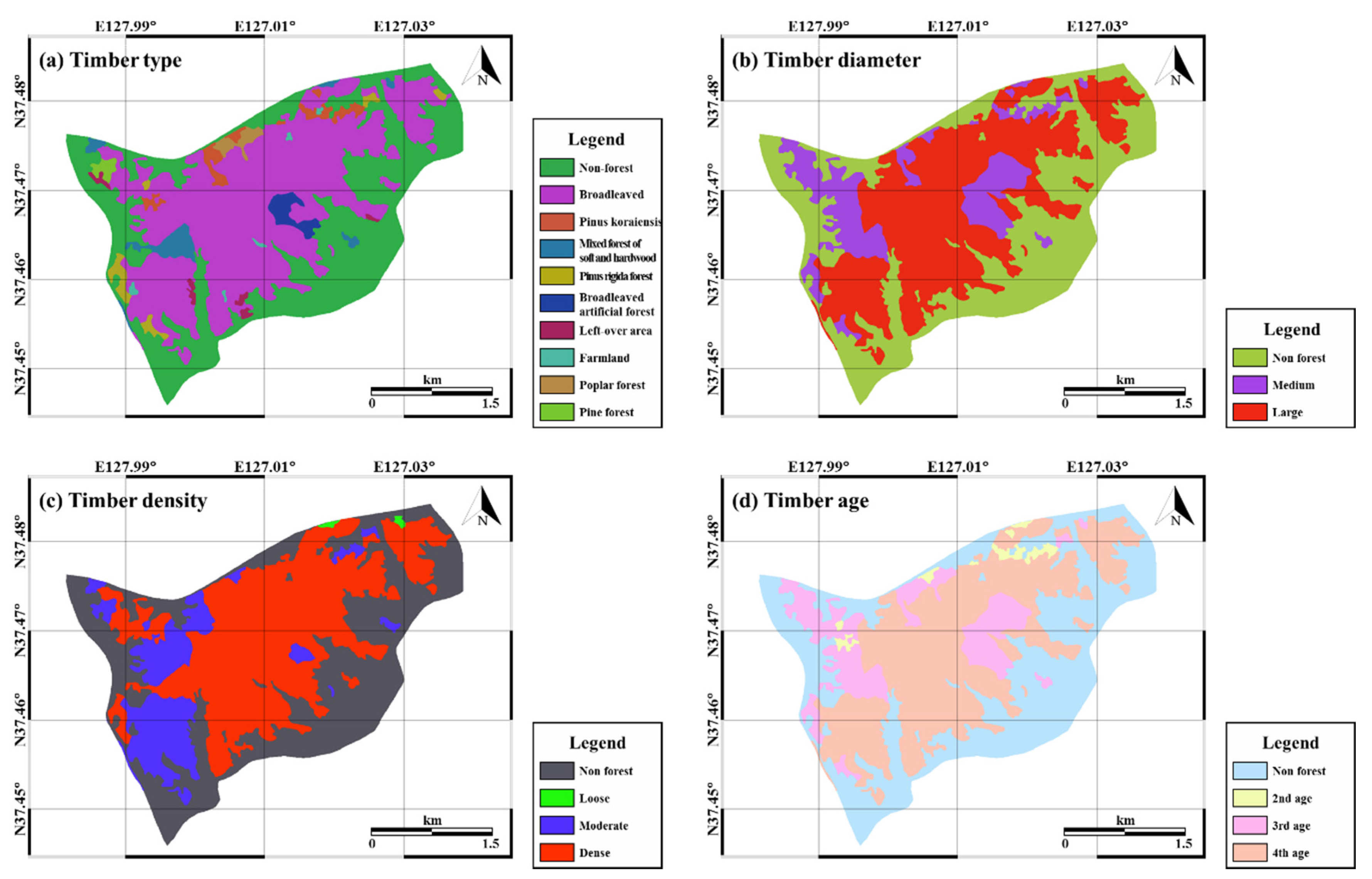
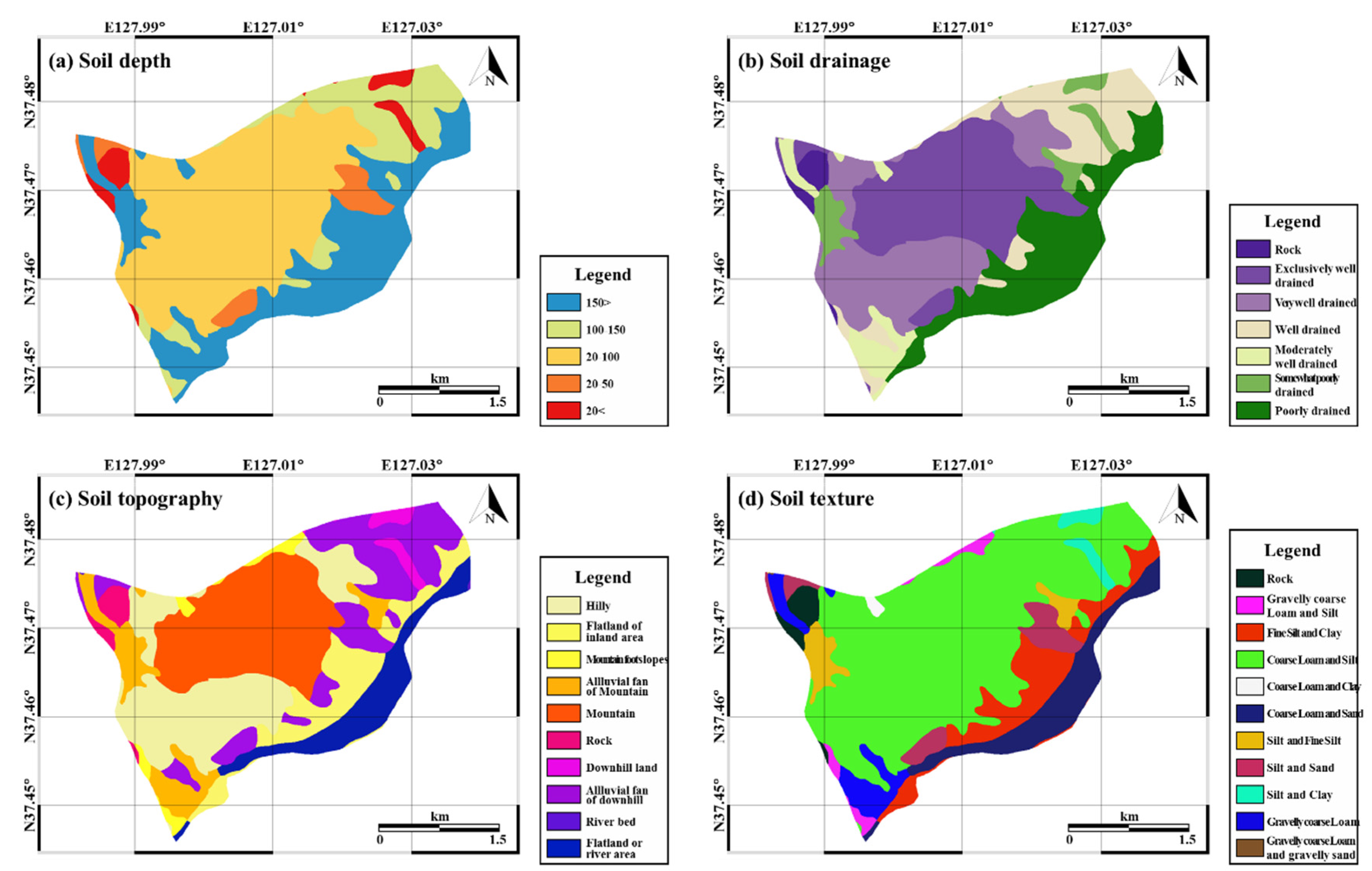
The type and composition of the soil influence the occurrence of landslides as they determine the degree of erosion and saturation [49]. The slope stability can be strengthened by the roots of vegetation and the degree of strengthening depends on the specific attributes of the vegetation; hence, the impact of heavy rainfall on the slope can be mitigated by vegetation [50]. The vegetation map was provided by the Korea Forest Research Institute and was in polygon format with a scale of 1:25,000 (Figure 4). The attributes of timber diameter, type, density, and age were extracted from the vegetation map. In addition to the vegetation variables, the soil type and condition also influence the occurrence of landslides. The soil maps used in this study were provided by the National Academy of Agricultural Science (RDA) in polygon format with a scale of 1:25,000. Soil depth, drainage, topography, and texture were derived from the soil maps (Figure 5).
All variables used in this study were resampled into a grid format of 5-m spatial resolution to create a spatial database. The total size of the spatial database was 1015 × 874, and the study area contained 457,133 cells. The 103 landslide occurrence locations in point format were also converted into the 5-m grid format to be included in the data in the spatial database. Half of the 103 landslide location data points (51 points) were used as training data, and the other half were used as validation data. All of the collected data were prepared in ASCII format from the grid. Finally, a spatial database was established to apply the model to (Table 1).
4. Methodology
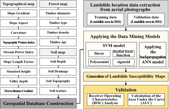
Landslides are affected by various factors and each element is simplified as input data in modeling studies. Given that natural phenomena such as landslides are composite events of each element, they should be analyzed using a modeling technique based on the relationships between data in a vast dataset such as a data mining model. Using data mining models, the relationships among all of the predisposing factors and the effects of all of the landslide-related factors on the model results can be analyzed. Therefore, in this study, the factors related to landslide susceptibility were used as the input data of the data mining models. The input variables were stored in a spatial database; 17 landslide-related variables were chosen from the spatial database, including half of the randomly selected landslide locations used as training data. Landslide susceptibility maps were created using two data mining models, specifically support vector machine (SVM) (Boulder, CO, USA) and ANN models, which are based on linear classifiers. Additionally, the weight of each factor was calculated in the data mining modeling process, and a validation was performed (Figure 6). A detailed description of the data mining models used in this study is given below.
4.1. Support Vector Machine
4.1.1. Basic Principles of SVM
The SVM method is a training algorithm based on nonlinear transformations that uses a classification based on the principle of structural risk minimization, which has performed well in the test phase [51]. When training data are represented in multidimensional space, several hyperplanes can be used to distinguish the data into two classes; however, there is only one optimum linear separating hyperplane [52]. This optimal hyperplane should maximize the distance between the data closest to the hyperplane. Thus, the objective of the SVM method is to determine a multi-dimensional hyperplane that differentiates the two classes with the maximum margin. The SVM model performs this process according to three main concepts: margin, support vector, and kernel.
The margin is the distance between a specific data point and the hyperplane that separates the data patterns. It is the shortest distance from the data vector of each class to the given hyperplane. The larger the margin, the more accurately the SVM model performs the classification; hence, the optimal hyperplane maximizes the margin when is the normal vector of the hyperplane, and is the norm of the normal of the hyperplane. is the norm of the normal of the hyperplane.
The hyperplane, which defines the two classes that maximize the margins when the data are linearly separable, can be defined by Equation (6). Under these conditions, the training data on these two hyperplanes constitute the support vector. Therefore, the support vector maintains the shortest distance to the hyperplane. The support vectors are dependable on the boundary of the hyperplane and they are time-efficient when a new dataset is tested with a support vector. The dataset of linear separable training vectors (i = 1, 2, …, n) and the training vectors consisting of two classes are represented by as the value of ±1 [53,54].
where b is the scalar base, and the scalar product operation is denoted by (·).
In addition, because the two hyperplanes must maximize the margin between them, the optimization of objective Equation (7) with the constraints of Equation (6) yields the planes of the two classes:
However, most cases do not satisfy the constraint as the data are not linearly separable. A formula including the slack variable indicates the distance from the hyperplane to the data located on the wrong side [52]; the penalty term C introduced to account for misclassification [55,56] was developed to address this problem.
4.1.2. SVM for Nonlinear Classification
In the preceding case of nonlinear boundary data, the SVM model is unable to generate an appropriate hyperplane. Therefore, the data can be classified into a linear problem as a hyperplane by mapping them to a high-dimensional space value from the low-dimensional data that cannot be linearly separated. To solve Equations (8) and (9) when the dataset is linearly separable, the training data are expressed as a vector inner product in the optimization process. This enables the inner product in the training algorithm to be expressed by the inner product of a function in a feature space when nonlinear data in the input space are mapped to a high-dimensional feature space by a specific function.
The hyperplane of the data with nonlinear data patterns can be derived by transforming the data space, but x cannot be computed directly; an arbitrary kernel function should be used to satisfy x [53]. The kernel functions, K(xi, xj), convert the original data into linearly separable data in high-dimensional feature space [52]. The kernel function should satisfy Mercer’s condition. The following four functions are the main kernel functions used in the SVM model:
where γ and d are parameters of the kernel functions.
In radial basis function (RBF) kernel, is the squared Euclidean distance between the vectors, and is defined as follows:
where is a freely adjustable parameter that controls the performance of the kernel, and r is a parameter of the sigmoid kernel.
In this study, the Environment for Visualizing Images (ENVI 5.0, Exelis Visual Information Solutions, Boulder, CO, USA) software program was used for the application of the SVM model (Boulder, CO, USA). The software provides four types of kernels in the SVM classifier as mentioned above: linear, polynomial, RBF, and sigmoid. Each kernel function has its own parameters, which should be adjusted appropriately according to the characteristics of the purpose. The default kernel of the ENVI software is the RBF kernel, which is known to provide more accurate prediction results in most classifications, particularly in nonlinear problems. After applying the kernel and classifying each input factor, the SVM model results were mapped using the process of overlapping and summation.
SVMall is the sum of all classification results by the SVM model for all variables, and SVMi is the single result of a given variable; in this study, the total number of input factors, n was 17. The results were mapped and validated using the landslide locations not used for training.
4.2. Artificial Neural Network
An ANN is a statistical learning algorithm that describes a neuronal signaling system. The human brain regulates the connection strength of synapses between neurons and determines whether signals are delivered or not; the ANN learns to derive the results with minimum error by adjusting the weight between input data and output data. The unit of the ANN is the perceptron, which is divided into an input layer and an output layer. The input layers are represented by nodes, which are linked to an edge having the weight of each node [57]. The model outputs 1 when the sum of the values of each layer multiplied by the weight is greater than or equal to the threshold; otherwise, the output is −1. This type of perceptron can only be applied to a linear classification and is not applicable in most cases.
In this study, multi-layered perceptrons allowing classification of nonlinear data were used with a hidden layer between the input and output layers. A feed-forward network was used for the map learning. The learning of neural networks progressed via a backpropagation algorithm that propagates the errors generated in the output layer to each layer and corrects the weights. In other words, the backpropagation algorithm learns the neural network by inverting the step, and the result most similar to the output layer value is derived based on the input layer. The process can be simplified as a combination of nodes and edges [58]. The backpropagation algorithm can be expressed by the following equation:
where is the updated weight for connection and is the learning rate. The initial value of weight is given randomly. is the error of the final output result when the expected output value is assumed to be , according to the input data [59].
where is the number assigned to the node in each layer, and is the number of output layers. Because the backpropagation algorithm updates the weights while propagating the error generated from the output to the input direction, it updates the weights starting from the portion from the output. is calculated repeatedly using the updated weight so as to be minimized; the differentiation of is fundamental. Therefore, when the calculated value is passed to the next layer or is expected to be the final result, an activation function is used to convert it to a range of values. In this study, a unipolar sigmoid function was used. The equation of the unipolar sigmoid function is as follows:
Using the activation function, the output value of each layer is adjusted from 0 to 1.
In this study, the ANN model was processed using MATLAB R2015a software (MathWorks, Massachusetts, MA, USA). Areas where the slope data were 0 were set as areas not prone to landslide occurrence and used for training data; landslide occurrence point data were also allocated to the training set. The backpropagation algorithm of the ANN was applied to estimate the weights between the input and the hidden layers, and between the hidden and the output layers by updating the hidden nodes and the learning rate. In this study, the input data were normalized to the range of 0.1–0.9 and a 17 × 34 × 1 structure was selected for the networks. The learning rate was set to 0.01 with a randomly selected initial weight. The number of epochs was set to 2000, and the root mean square error value was set to 0.1, which was used for the stopping criterion.
5. Results
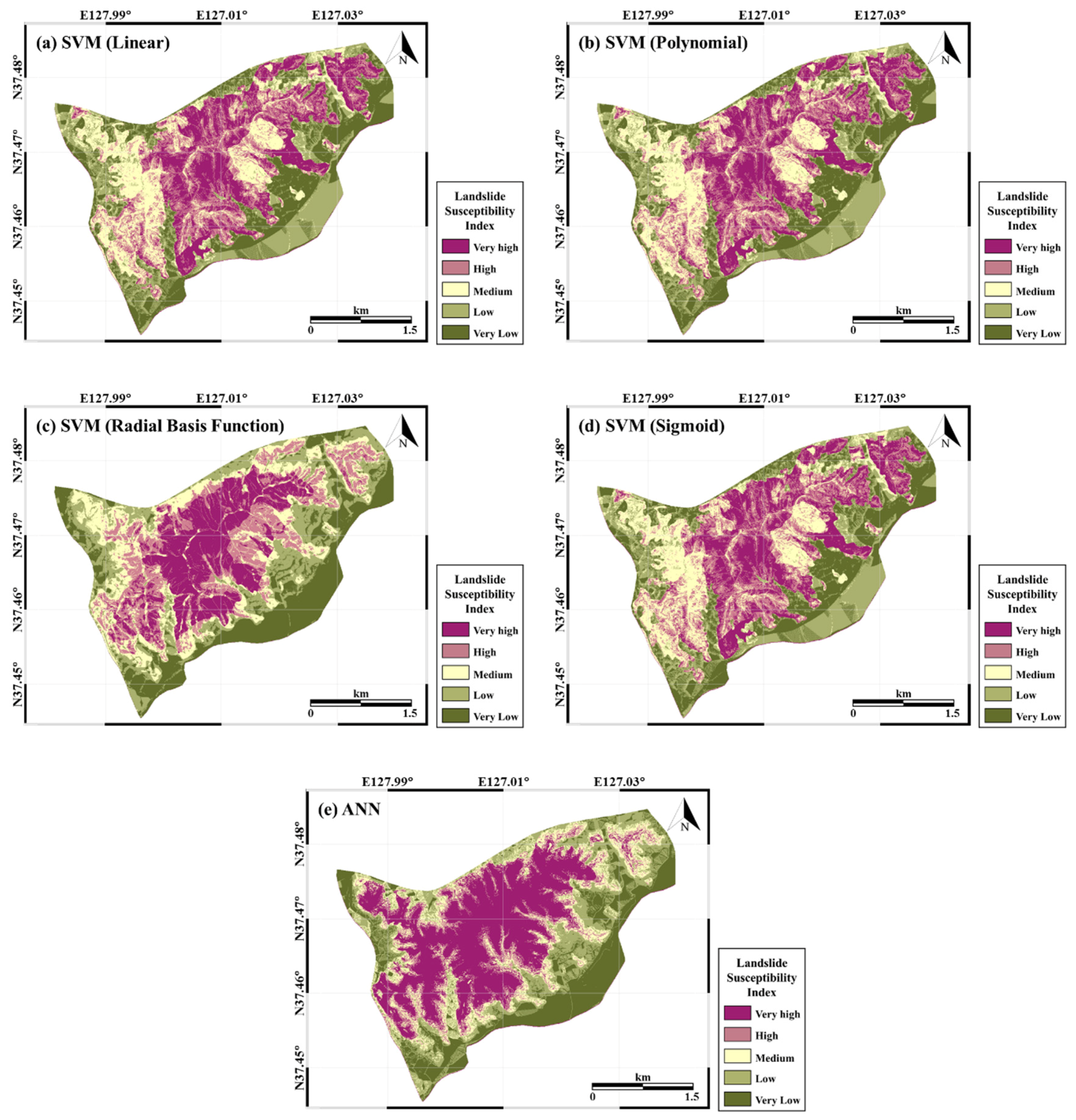
Figure 7a–d shows the landslide susceptibility maps produced by applying the SVM models with four kernels; and Figure 7e shows the map of the results from the ANN models. The values of the landslide susceptibility results were sorted in descending order and categorized into five classes for easy visual interpretation. For intuitive and efficient analysis, the results for the landslide susceptible areas were classified into five groups of approximately the same size: very high, high, medium, low, and very low susceptibility. The comparative analysis between the results and existing landslide occurrence locations was also made easier by representing the landslide susceptibility with the five categories. The spatial distribution of the landslide locations was concentrated in high-susceptibility areas.
In Figure 7, the results map of the linear, polynomial, and sigmoid kernels of the SVM models showed a similar pattern and represented the influence of the input factors of Figure 4 and Figure 5. In addition, the RBF kernel showed a similar pattern to the ANN map in that the center of the map had relatively higher susceptibility. In general, highly susceptible areas were principally distributed in the northeast direction from the center of the study area. Areas with high susceptibility were located in dense forest areas of broadleaved forest, above-average soil depth, and steep slopes. The dominant rocks constituting the Umyeonsan area are gneissic rocks, which have high landslide susceptibility because they are heavily eroded; landslides occur in areas of high soil drainage.
In Table 2, the area of each class is represented by percentage. The areas with very high indices in the SVM model were 2.2599, 2.2599, 2.2889 and 2.28369 km2 for the linear, polynomial, RBF, and sigmoid kernels, respectively. Among the results from the SVM models, the RBF kernel accounted for a slightly higher percentage (20.03%) of the areas with a very high index compared with the linear, polynomial, and sigmoid kernels. The areas with a very high index in the ANN model covered 3.9262 km2, which had the highest percentage (34.35%). In contrast, the areas with high index accounted for only a small proportion (8.65%). The area with a very low index accounted for similar percentages of 20.00, 20.00, 20.00 and 19.99% for the linear, polynomial, and sigmoid kernels, and ANN, respectively, while the RBF accounted for a lower percentage of 19.89%.
Table 3 shows the relative weights per variable, which were calculated from randomly selected training data for 20 epochs of 200 cycles. The weights between layers represent the contribution of each variable to the prediction of the landslide susceptibility. Timber age showed the lowest average value of weight, 0.04828. For the comparison analysis of the relativeness of the weights, the values were divided by the weight of the timber age and were normalized with respect to the average weight of the timber age. The highest average weight of 0.09615 for the standardized height was normalized to 2.00164, which was approximately twice the value of the weight of the timber age. The second major variable contributing to landslides was timber diameter (1.46886), followed by curvature (1.28335), soil depth (1.27746), and aspect (1.25804). The standard deviation ranged from 0.00022 to 0.01132.
To investigate the reliability of the proposed landslide susceptibility map using the previously described SVM and ANN data mining models, we performed a validation. The 2011 landslide occurrence data not used for the training were used for validation. After 51 points of training data had been extracted using random sampling from the landslide occurrence data from the 2011 Umyeonsan landslide and applied to the models, 52 points were used for the validation. Because the predicted landslide susceptibility map was an indicator of the potential possibility of landslides in the future, the data obtained after the occurrence of the landslides were a suitable choice for the validation data. However, an erosion control project implemented after the 2011 event has significantly reduced the possibility of landslides. Therefore, it is important to obtain information on landslide susceptibility in areas where landslides have not occurred. In addition, implementation of precautionary measures to prevent landslides from occurring in the future is necessary. Thus, half of the landslide occurrence points were used as training data, and the remaining points were used as validation data.
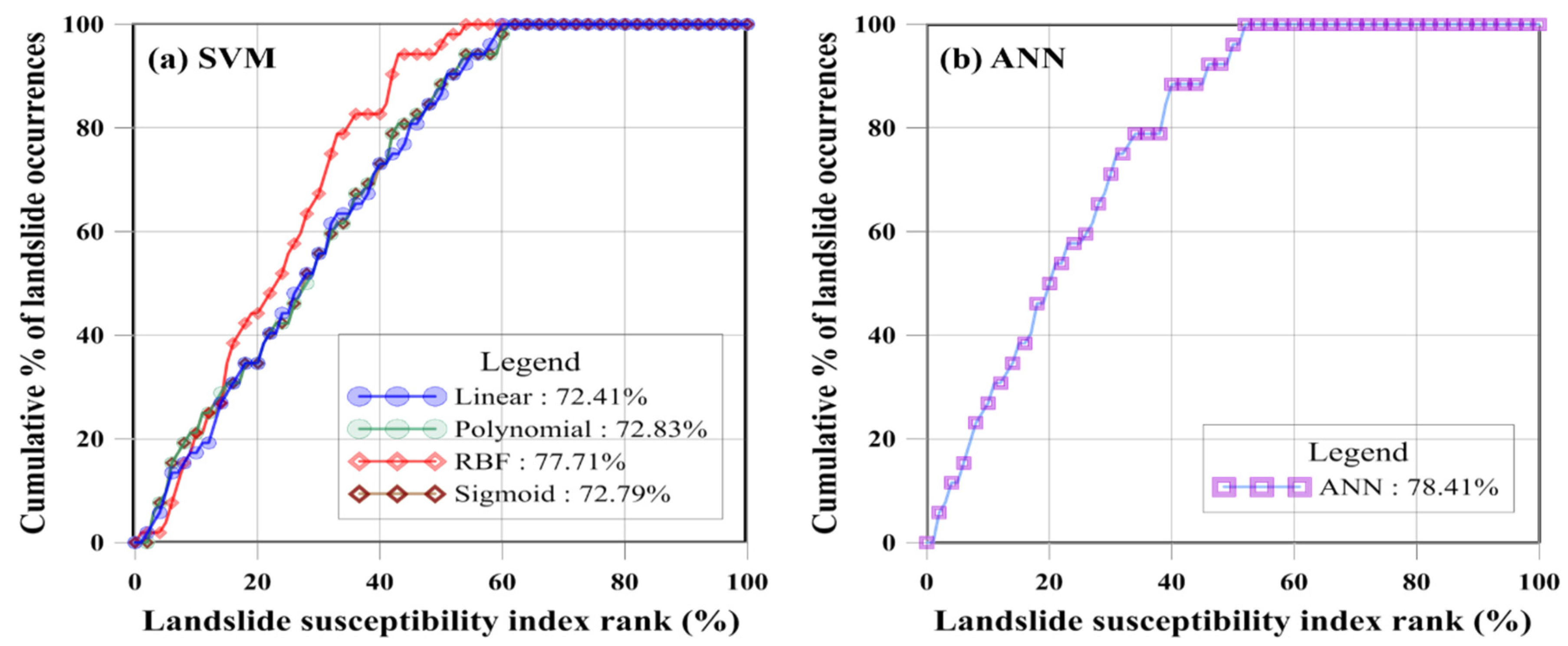
The AUC of the receiver operating characteristic (ROC) curve was used for the validation of the models. The ROC consists of specificity, the x-axis, which shows the percentage of the areas where landslides are expected to occur but have not occurred, and sensitivity, the y-axis, which represents the predicted landslide areas according to training data of landslide occurrences. The ROC graph was drawn using the following procedure. To show the rank relative to the predicted results, the values of the results of landslide susceptibility from the models were sorted in descending order. The ranked results were represented in ROC curves using 100 classes; a single class comprised an area that was approximately 1% of the total study area. Figure 8a shows the AUC of the landslide susceptibility map for the SVM model; the linear, polynomial, RBF, and sigmoid kernel had 72.41 (0.7241), 72.83 (0.7283), 77.17 (0.7717) and 72.79% (0.7279) accuracy versus 78.41% (0.7841) accuracy in the ANN model (Figure 8b).
A higher AUC value indicates better model performance, but it is important to perform additional empirical analyses based on input and ground truth data. Our validation results indicated that the five landslide sensitivity assessments performed well; the AUC values were all greater than 0.7 [60]. In the SVM model, the AUC value using the RBF kernel was 0.7717, which was superior to the other three kernels in the study area. The ANN model yielded an AUC value of 0.7841, which was approximately 6% higher than that of the SVM model with the linear kernel, and 0.7% higher than with the RBF kernel. The graphs of the validation results are depicted in Figure 8; in all of the models, 60% of the study area incorporated all of the landslide locations.
6. Discussion
In this study, two types of data mining models were used to create landslide susceptibility maps. Because the results of data mining models are derived from their data, the reliability of the input data is fundamental. Landslide location data were acquired from aerial photographs to provide accurate training datasets. The data mining models are suitable for observing the rapid changes in an urban area with its compactness and complex characteristics. In addition, other topographical-, forest-, and soil-related variables were obtained, and topographic-related factors were calculated from the topographical map produced from the aerial photographs.
The results from each model in Figure 7 were not statistically different in the spatial pattern of the landslide susceptibility area. This can be interpreted that all of the four prediction results from the SVM model were based on the same input factors, and all landslide predisposing factors were regarded as having equal importance so that the same weight was assigned to each predisposing factor. However, for the results from the RBF kernel, which had the highest accuracy among the SVM models, the susceptibility on the west, southwest, and southeast slopes was lower than that from the other kernels, which was similar to the trend for the ANN model. In general, the northern area of the mountain showed high susceptibility, and had the same pattern as the existing damaged area of the southern ring roads.
The percentages of the classes of five indices were also calculated. The linear, polynomial, and sigmoid kernels were distributed fairly evenly, while the RBF kernel showed a slightly higher percentage in the very high index class, and a lower percentage in the very low index class. This suggests that a high percentage in the high susceptibility index yields good validation results. Figure 8a shows that the RBF kernel had a percentage of 77.71%, which was approximately 5% higher than that of the other kernels. Similarly, the results from the ANN model yielded a high percentage (more than 30% of the total) in the very high class, which represented high risk areas, and this also led to a high validation percentage for the ANN model, 78.41%. In addition, the ANN model results in Table 3 show that the standardized height contributed most to landslide susceptibility with a normalized weight of greater than 2. This can be seen in Figure 7e, which shows the effect of standardized height with the high relative weight of the ANN model. Standardized height was the most important factor among all of the landslide-related factors. The factors related to landslide susceptibility should be managed based on their relative weight.
Because this study investigated the susceptibility of landslides in urban areas, the study area was fairly small, with an area of approximately 11.4 km2 and a spatial resolution of 5 m along road and river boundaries rather than a rectangular boundary. It should be noted that the ROC was characterized using a percentage of the landslide susceptibility rates. Thus, in this study, the validation rate was relatively low compared with most previous studies, which were based on rectangles. Moreover, we could use the slope unit instead of common raster unit, which is closely correlated to the topography, for the further steps; the slope unit is defined as the unit between the valleys and ridges. Most of the mountains in the city are managed in the framework of city parks in which the various economic and social aspects of Umyeonsan are also considered, rather than the area being covered solely by forests that are more resistant to landslides. Given that landslide damage in urban areas can lead to human casualties, it is important to investigate the soil and topographical characteristics of the areas where landslides are likely to occur. Furthermore, landslide risk should be incorporated in city-level policies.
7. Conclusions
In this study, we applied a spatial data mining approach to identify areas where landslides are likely to occur using aerial photographs and GIS. Landslide-prone locations were determined using the interpretation of aerial photographs and field survey results to construct spatial datasets. The topographical predisposing factors were extracted from a digital topographical map constructed from aerial photographs, and the soil and forest predisposing factors were extracted from publicly available maps. A spatial database was constructed using the extracted and calculated factors including randomly extracted training data for the landslide area, and landslide susceptibility was mapped using SVM and ANN models. Finally, the results map was validated using the half of the landslide location data not used for training.
In urban areas such as Seoul, landslides have previously not been considered a serious concern, compared with floods and storms. Seoul has undergone rapid urbanization that has taken place with little consideration of natural disasters. In large cities such as Seoul, global warming, rapid urbanization, extreme precipitation, and population pressures could potentially lead to complex events, including landslides occurring in the city, which could have serious consequences. Therefore, it is important to create a scientifically valid landslide susceptibility map for urban areas such as Seoul.
The predicted rate of landslides was high on the steep mountain tops and similar to the general landslide pattern on the ridges. The map created in this study showed that susceptibility to landslides decreased with slope gradient. Because landslides are caused by differences in gravity due to terrain shape, it is logical that their occurrence is affected by the geographical structure of the area. The relationship between landslide occurrence and forested land cover showed that broadleaved forests had a high susceptibility, and this type of forest occupied the largest proportion of the study area. In addition, large trunk-size, high-density forests, and middle-aged forests had a high risk of landslides. Among the soil factors, red and yellow soils had higher landslide susceptibility, as well as areas with large soil depth; the occurrence rate was higher in areas with good soil drainage. The performance of the SVM and ANN models was validated using AUC analysis. The SVM model yielded 72.41%, 72.83%, 77.17% and 72.79% accuracy for the linear, polynomial, RBF, and sigmoid kernels, respectively; while the ANN model had 78.41% accuracy. The results of this study are expected to support spatial decision-making from relevant agencies to formulate policies related to landslide disaster risk reduction in urban areas.
Acknowledgments
This research was conducted by Korea Environment Institute (KEI) with support of a grant (16CTAP-C114629-01) from Technology Advancement Research Program (TARP) funded by Ministry of Land, Infrastructure and Transport of Korean government. This work was supported by the Space Core Technology Development Program through the National Research Foundation of Korea, funded by the Ministry of Science, ICT and Future Planning, under Grant (NRF-2014M1A3A3A03034798).
Author Contributions
Sunmin Lee applied the SVM and ANN models and wrote the paper. Hyung-Sup Jung designed the experiments. Also, he interpreted the input data and the results. Moung-Jin Lee suggested the idea and organized the paperwork. In addition, he collected data and conducted pre-processing of the input data. All of authors contributed to the writing of each part.
Conflicts of Interest
The authors declare no conflict of interest.
References
- Berry, M.J.; Linoff, G. Data Mining Techniques: For Marketing, Sales, and Customer Support; John Wiley & Sons, Inc.: Hoboken, NJ, USA, 1997. [Google Scholar]
- Pachauri, R.K.; Allen, M.R.; Barros, V.R.; Broome, J.; Cramer, W.; Christ, R.; Church, J.A.; Clarke, L.; Dahe, Q.; Dasgupta, P. Contribution of working groups I, II and III to the fifth assessment report of the intergovernmental panel on climate change. In Climate Change 2014: Synthesis Report; IPCC: Geneva, Switzerland, 2014. [Google Scholar]
- Centre for Research on the Epidemiology of Disasters, UN Office for Disaster Risk Reduction. The Human Cost of Natural Disasters: A Global Perspective; Centre for Research on the Epidemiology of Disaster (CRED): Brussels, Belgium, 2015. [Google Scholar]
- Cruden, D.; Varnes, D. Landslide Types and Processes. In Landslides: Investigation and Mitigation; Turner, A.K., Schuster, R.L., Eds.; Special Report 247; Transportation Research Board: Washington, DC, USA, 1996; pp. 36–75. [Google Scholar]
- Choi, J.; Oh, H.J.; Lee, H.J.; Lee, C.; Lee, S. Combining landslide susceptibility maps obtained from frequency ratio, logistic regression, and artificial neural network models using aster images and gis. Eng. Geol. 2012, 124, 12–23. [Google Scholar] [CrossRef]
- Lee, S.; Ryu, J.H.; Won, J.S.; Park, H.J. Determination and application of the weights for landslide susceptibility mapping using an artificial neural network. Eng. Geol. 2004, 71, 289–302. [Google Scholar] [CrossRef]
- Pradhan, B.; Lee, S. Landslide susceptibility assessment and factor effect analysis: Backpropagation artificial neural networks and their comparison with frequency ratio and bivariate logistic regression modelling. Environ. Model. Softw. 2010, 25, 747–759. [Google Scholar] [CrossRef]
- Pradhan, B.; Lee, S. Utilization of optical remote sensing data and gis tools for regional landslide hazard analysis using an artificial neural network model. Earth Sci. Front. 2007, 14, 143–151. [Google Scholar]
- Ahmed, B.; Dewan, A. Application of bivariate and multivariate statistical techniques in landslide susceptibility modeling in chittagong city corporation, bangladesh. Remote Sens. 2017, 9. [Google Scholar] [CrossRef]
- Lee, S. Application of logistic regression model and its validation for landslide susceptibility mapping using gis and remote sensing data. Int. J. Remote Sens. 2005, 26, 1477–1491. [Google Scholar] [CrossRef]
- Scaioni, M.; Longoni, L.; Melillo, V.; Papini, M. Remote sensing for landslide investigations: An overview of recent achievements and perspectives. Remote Sens. 2014, 6, 9600–9652. [Google Scholar] [CrossRef]
- Akcay, O. Landslide fissure inference assessment by anfis and logistic regression using uas-based photogrammetry. ISPRS Int. J. Geo-Inf. 2015, 4, 2131–2158. [Google Scholar] [CrossRef]
- Bui, D.T.; Pradhan, B.; Lofman, O.; Revhaug, I.; Dick, O.B. Landslide susceptibility assessment in the hoa binh province of vietnam: A comparison of the levenberg–marquardt and bayesian regularized neural networks. Geomorphology 2012, 171, 12–29. [Google Scholar]
- Yilmaz, I. Landslide susceptibility mapping using frequency ratio, logistic regression, artificial neural networks and their comparison: A case study from kat landslides (Tokat—Turkey). Comput. Geosci. 2009, 35, 1125–1138. [Google Scholar] [CrossRef]
- Ermini, L.; Catani, F.; Casagli, N. Artificial neural networks applied to landslide susceptibility assessment. Geomorphology 2005, 66, 327–343. [Google Scholar] [CrossRef]
- Pourghasemi, H.R.; Pradhan, B.; Gokceoglu, C. Application of fuzzy logic and analytical hierarchy process (ahp) to landslide susceptibility mapping at haraz watershed, iran. Nat. Hazards 2012, 63, 965–996. [Google Scholar] [CrossRef]
- Pradhan, B. Use of gis-based fuzzy logic relations and its cross application to produce landslide susceptibility maps in three test areas in malaysia. Environ. Earth Sci. 2011, 63, 329–349. [Google Scholar] [CrossRef]
- Bai, S.; Lü, G.; Wang, J.; Zhou, P.; Ding, L. Gis-based rare events logistic regression for landslide-susceptibility mapping of lianyungang, china. Environ. Earth Sci. 2011, 62, 139–149. [Google Scholar] [CrossRef]
- Gorsevski, P.V.; Gessler, P.E.; Foltz, R.B.; Elliot, W.J. Spatial prediction of landslide hazard using logistic regression and roc analysis. Trans. GIS 2006, 10, 395–415. [Google Scholar] [CrossRef]
- Pradhan, B.; Mansor, S.; Pirasteh, S.; Buchroithner, M.F. Landslide hazard and risk analyses at a landslide prone catchment area using statistical based geospatial model. Int. J. Remote Sens. 2011, 32, 4075–4087. [Google Scholar] [CrossRef]
- Rawat, M.; Joshi, V.; Rawat, B.; Kumar, K. Landslide movement monitoring using gps technology: A case study of bakthang landslide, gangtok, east sikkim, india. J. Dev. Agric. Econ. 2011, 3, 194–200. [Google Scholar]
- Hess, D.M.; Leshchinsky, B.A.; Bunn, M.; Mason, H.B.; Olsen, M.J. A simplified three-dimensional shallow landslide susceptibility framework considering topography and seismicity. Landslides 2017, 08, 1–21. [Google Scholar] [CrossRef]
- Lee, S.; Chwae, U.; Min, K. Landslide susceptibility mapping by correlation between topography and geological structure: The janghung area, korea. Geomorphology 2002, 46, 149–162. [Google Scholar] [CrossRef]
- Zhou, S.; Chen, G.; Fang, L. Distribution pattern of landslides triggered by the 2014 ludian earthquake of china: Implications for regional threshold topography and the seismogenic fault identification. ISPRS Int. J. Geo-Inf. 2016, 5. [Google Scholar] [CrossRef]
- Devkota, K.C.; Regmi, A.D.; Pourghasemi, H.R.; Yoshida, K.; Pradhan, B.; Ryu, I.C.; Dhital, M.R.; Althuwaynee, O.F. Landslide susceptibility mapping using certainty factor, index of entropy and logistic regression models in gis and their comparison at mugling–narayanghat road section in nepal himalaya. Nat. Hazards 2013, 65, 135–165. [Google Scholar] [CrossRef]
- Korea Forest Service. 2013 Detailed Strategy for Primary Policy; Korea Forest Service: Seoul, Korea, 2013; pp. 12–16.
- Lee, M.; Park, I.; Won, J.; Lee, S. Landslide hazard mapping considering rainfall probability in inje, Korea. Geomat. Nat. Hazards Risk 2016, 7, 424–446. [Google Scholar] [CrossRef]
- Lee, S.; Hong, S.M.; Jung, H.S. A support vector machine for landslide susceptibility mapping in Gangwon Province, Korea. Sustainability 2017, 9. [Google Scholar] [CrossRef]
- Park, I.; Lee, S. Spatial prediction of landslide susceptibility using a decision tree approach: A case study of the pyeongchang area, Korea. Int. J. Remote Sens. 2014, 35, 6089–6112. [Google Scholar] [CrossRef]
- Lee, S.; Min, K. Statistical analysis of landslide susceptibility at yongin, Korea. Environ. Geol. 2001, 40, 1095–1113. [Google Scholar] [CrossRef]
- Lee, S.; Evangelista, D. Landslide Susceptibility Mapping Using Probability and Statistics Models in Baguio City, Philippines; Department of Environment and Natural Resources: Quezon City, Philippines, 2008.
- Lee, S.; Pradhan, B. Landslide hazard assessment at cameron highland malaysia using frequency ratio and logistic regression models. Geophys. Res. Abstr. 2006, 8. SRef-ID: 1607-7962/gra/EGU06-A-003241. [Google Scholar]
- Oh, H.-J.; Lee, S.; Soedradjat, G.M. Quantitative landslide susceptibility mapping at pemalang area, Indonesia. Environ. Earth Sci. 2010, 60, 1317–1328. [Google Scholar] [CrossRef]
- Bathrellos, G.D.; Gaki-Papanastassiou, K.; Skilodimou, H.D.; Papanastassiou, D.; Chousianitis, K.G. Potential suitability for urban planning and industry development using natural hazard maps and geological–geomorphological parameters. Environ. Earth Sci. 2012, 66, 537–548. [Google Scholar] [CrossRef]
- Bathrellos, G.D.; Skilodimou, H.D.; Chousianitis, K.; Youssef, A.M.; Pradhan, B. Suitability estimation for urban development using multi-hazard assessment map. Sci. Total Environ. 2017, 575, 119–134. [Google Scholar] [CrossRef] [PubMed]
- Chousianitis, K.; Del Gaudio, V.; Sabatakakis, N.; Kavoura, K.; Drakatos, G.; Bathrellos, G.D.; Skilodimou, H.D. Assessment of earthquake-induced landslide hazard in greece: From arias intensity to spatial distribution of slope resistance demand. Bull. Seismol. Soc. Am. 2016, 106, 174–188. [Google Scholar] [CrossRef]
- Papadopoulou-Vrynioti, K.; Bathrellos, G.D.; Skilodimou, H.D.; Kaviris, G.; Makropoulos, K. Karst collapse susceptibility mapping considering peak ground acceleration in a rapidly growing urban area. Eng. Geol. 2013, 158, 77–88. [Google Scholar] [CrossRef]
- Korean Geotechnical Society. Cause Investigation of Umyeonsan Landslide and Recovery Measure Establishment Service Final Report; Korean Geotechnical Society: Seoul, Korea, 2011; p. 3. [Google Scholar]
- Seoul Special City. Supplemental Investigation Report of Causes of Umyeonsan Landslides; Seoul Special City: Seoul, Korea, 2014; p. 447. [Google Scholar]
- Nocutnews. A Part of Umyeonsan. Available online: http://news.Naver.Com/main/read.Nhn?Mode=lsd&mid=sec&sid1=102&oid=079&aid=0002273090 (accessed on 20 June 2017).
- SBS. An Approval of a mAn-Made Disaster, Not a Natural Disaster, Umyeonsan Landslide. Available online: http://news.Sbs.Co.Kr/news/endpage.Do?News_id=n1002292872&plink=oldurl (accessed on 20 June 2017).
- Jones, D.; Brunsden, D.; Goudie, A. A preliminary geomorphological assessment of part of the karakoram highway. Q. J. Eng. Geol. Hydrogeol. 1983, 16, 331–355. [Google Scholar] [CrossRef]
- Beven, K.; Kirkby, M.J. A physically based, variable contributing area model of basin hydrology/un modèle à base physique de zone d’appel variable de l’hydrologie du bassin versant. Hydrol. Sci. J. 1979, 24, 43–69. [Google Scholar] [CrossRef]
- Moore, I.D.; Grayson, R.; Ladson, A. Digital terrain modelling: A review of hydrological, geomorphological, and biological applications. Hydrol. Process. 1991, 5, 3–30. [Google Scholar] [CrossRef]
- Wischmeier, W.H.; Smith, D.D. Predicting Rainfall Erosion Losses—A Guide to Conservation Planning; U.S. Department of Agriculture: Washington, DC, USA, 1978.
- Conrad, O.; Bechtel, B.; Bock, M.; Dietrich, H.; Fischer, E.; Gerlitz, L.; Wehberg, J.; Wichmann, V.; Böhner, J. System for automated geoscientific analyses (saga) v. 2.1.4. Geosci. Model Dev. 2015, 8, 1991–2007. [Google Scholar] [CrossRef]
- Böhner, J.; Selige, T. Spatial prediction of soil attributes using terrain analysis and climate regionalisation. Gottinger Geographische Abhandlungen 2006, 115, 13–28. [Google Scholar]
- Hjerdt, K.; McDonnell, J.; Seibert, J.; Rodhe, A. A new topographic index to quantify downslope controls on local drainage. Water Resour. Res. 2004, 40, W05601–W05606. [Google Scholar] [CrossRef]
- Doetterl, S.; Berhe, A.A.; Nadeu, E.; Wang, Z.; Sommer, M.; Fiener, P. Erosion, deposition and soil carbon: A review of process-level controls, experimental tools and models to address c cycling in dynamic landscapes. Earth-Sci. Rev. 2016, 154, 102–122. [Google Scholar] [CrossRef]
- Anthes, R.A. Enhancement of convective precipitation by mesoscale variations in vegetative covering in semiarid regions. J. Clim. Appl. Meteorol. 1984, 23, 541–554. [Google Scholar] [CrossRef]
- Choi, J.W.; Byun, Y.G.; Kim, Y.I.; Yu, K.Y. Support vector machine classification of hyperspectral image using spectral similarity kernel. J. Korea Soc. Geospat. Inf. Sci. 2006, 14, 71–77. [Google Scholar]
- Cortes, C.; Vapnik, V. Support-vector networks. Mach. Learn. 1995, 20, 273–297. [Google Scholar] [CrossRef]
- Yao, X.; Tham, L.; Dai, F. Landslide susceptibility mapping based on support vector machine: A case study on natural slopes of Hong Kong, China. Geomorphology 2008, 101, 572–582. [Google Scholar] [CrossRef]
- Xu, C.; Dai, F.; Xu, X.; Lee, Y.H. Gis-based support vector machine modeling of earthquake-triggered landslide susceptibility in the jianjiang river watershed, China. Geomorphology 2012, 145, 70–80. [Google Scholar] [CrossRef]
- Zhu, J.; Hastie, T. Kernel logistic regression and the import vector machine. J. Comput. Graph. Stat. 2005, 14, 185–205. [Google Scholar] [CrossRef]
- Schölkopf, B.; Smola, A.J.; Williamson, R.C.; Bartlett, P.L. New support vector algorithms. Neural Comput. 2000, 12, 1207–1245. [Google Scholar] [CrossRef] [PubMed]
- Atkinson, P.M.; Tatnall, A. Introduction neural networks in remote sensing. Int. J. Remote Sens. 1997, 18, 699–709. [Google Scholar] [CrossRef]
- Magoulas, G.D.; Vrahatis, M.N.; Androulakis, G.S. Effective backpropagation training with variable stepsize. Neural Netw. 1997, 10, 69–82. [Google Scholar] [CrossRef]
- Hines, J.; Tsoukalas, L.H.; Uhrig, R.E. Matlab Supplement to Fuzzy and Neural Approaches in Engineering; John Wiley & Sons, Inc.: Hoboken, NJ, USA, 1997. [Google Scholar]
- Fawcett, T. An introduction to roc analysis. Pattern Recognit. Lett. 2006, 27, 861–874. [Google Scholar] [CrossRef]
Figure 1.
Map showing the location of the study area of Umyeonsan: (a) South Korea; (b) Seoul; and (c) Umyeonsan.
Figure 1.
Map showing the location of the study area of Umyeonsan: (a) South Korea; (b) Seoul; and (c) Umyeonsan.
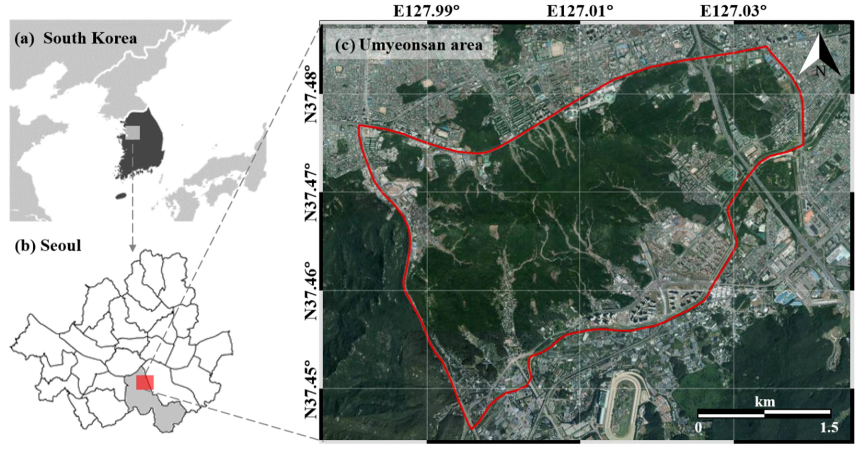
Figure 2.
Data of landslide occurrence locations from aerial photographs: (a) before landslides in 2011; (b) after landslides in 2011; (c) training and validation data; (d) damage situation in Southern Circular Road [40]; (e) Gyungnam apartment buildings in Seocho-gu [41].

Figure 3.
Topographical factors related to landslides used to construct a spatial database: (a) slope gradient; (b) slope aspect; (c) curvature; (d) topographic wetness index (TWI); (e) stream power index (SPI); (f) slope length factor (SLF); (g) standardized height; (h) valley depth; (i) downslope distance gradient.

Figure 4.
Landslide-related factors obtained from the vegetation map: (a) timber type; (b) timber diameter; (c) timber density; (d) timber age.
Figure 4.
Landslide-related factors obtained from the vegetation map: (a) timber type; (b) timber diameter; (c) timber density; (d) timber age.

Figure 5.
Landslide-related factors obtained from the soil map: (a) soil depth; (b) soil drainage; (c) soil topography; (d) soil texture.
Figure 5.
Landslide-related factors obtained from the soil map: (a) soil depth; (b) soil drainage; (c) soil topography; (d) soil texture.

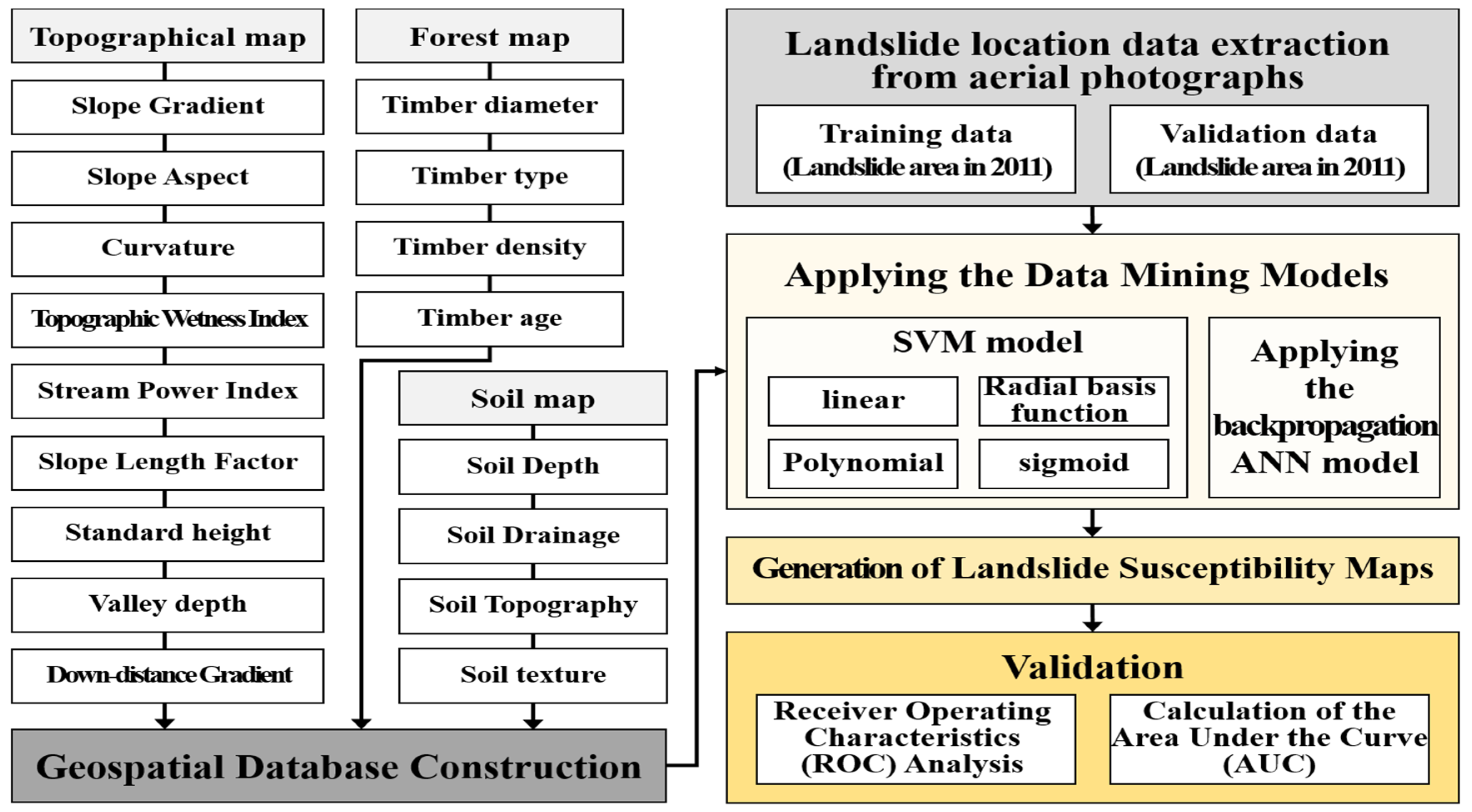
Figure 6.
Flowchart of the spatial prediction of landslide susceptibility.

Figure 7.
Landslide susceptibility maps generated using data mining models: Using an (a) support vector machine (SVM) model with linear kernel; (b) SVM model with polynomial kernel; (c) SVM model with radial basis function kernel; (d) SVM model with sigmoid kernel; (e) and the artificial neural network (ANN) model.

Figure 8.
Validation results using data mining models: (a) SVM model; (b) ANN model.


Table 1.
Landslide-related factors used to construct spatial database.
| Original Data | Factors | Data Type | Scale |
|---|---|---|---|
| Aerial photograph | Landslide location | Point | 1:1000 |
| Topographical map a | Slope gradient [°] Slope aspect Curvature Topographic Wetness Index (TWI) Stream Power Index (SPI) Slope Length Factor (SLF) Standardized height [m] Valley depth [m] Downslope distance gradient [rad] | GRID | 1:1000 |
| Forest map b | Timber diameter Timber type Timber density Timber age | Polygon | 1:25,000 |
| Soil map c | Soil depth Soil drainage Soil Topography Soil texture | Polygon | 1:25,000 |
a Topographical factors were extracted from digital topographic map by National Geographic Information Institute; b The forest map produced by Korea Forest Service; c The detailed soil map produced by Rural Development Administration
Table 2.
Area and percentage of each category.
| Landslide Susceptibility Index | SVM | Backpropagation ANN (km2) | Percentage (%) | |||||||
|---|---|---|---|---|---|---|---|---|---|---|
| Linear (km2) | Percentage (%) | Polynomial (km2) | Percentage (%) | RBF (km2) | Percentage (%) | Sigmoid (km2) | Percentage (%) | |||
| Very high | 2.2599 | 19.77% | 2.2599 | 19.77% | 2.2889 | 20.03% | 2.2836 | 19.98% | 3.9262 | 34.35% |
| High | 2.3081 | 20.20% | 2.3081 | 20.20% | 2.1835 | 19.11% | 2.2866 | 20.01% | 0.9881 | 8.65% |
| Moderate | 2.2878 | 20.02% | 2.2878 | 20.02% | 2.2359 | 19.56% | 2.2863 | 20.01% | 1.9451 | 17.02% |
| Low | 2.2866 | 20.01% | 2.2866 | 20.01% | 2.4474 | 21.41% | 2.2859 | 20.00% | 2.2849 | 19.99% |
| Very low | 2.2858 | 20.00% | 2.2858 | 20.00% | 2.2727 | 19.89% | 2.2859 | 20.00% | 2.2841 | 19.99% |
| Total | 11.4283 | 100.00 | 11.4283 | 100.00 | 11.4283 | 100.00 | 11.4283 | 100.00 | 11.4283 | 100.00 |
Table 3.
Neural network weight between landslide and related factors.
| 200 Cycles for 1 epoch | 1 | 2 | 3 | 4 | 5 | 6 | 7 | 8 | 9 | 10 | Average | Standard Deviation | Normalized Weight with Respect to Timber Age |
|---|---|---|---|---|---|---|---|---|---|---|---|---|---|
| Slope gradient | 0.0555 | 0.0548 | 0.0546 | 0.0546 | 0.0549 | 0.0552 | 0.0557 | 0.0561 | 0.0564 | 0.0567 | 0.05545 | 0.00072 | 1.14851 |
| Slope aspect | 0.0616 | 0.0611 | 0.0608 | 0.0607 | 0.0607 | 0.0606 | 0.0606 | 0.0605 | 0.0604 | 0.0603 | 0.06073 | 0.00036 | 1.25787 |
| Curvature | 0.0623 | 0.0615 | 0.0614 | 0.0615 | 0.0616 | 0.0618 | 0.0620 | 0.0623 | 0.0625 | 0.0629 | 0.06198 | 0.00048 | 1.28376 |
| TWI | 0.0512 | 0.0520 | 0.0512 | 0.0506 | 0.0500 | 0.0495 | 0.0490 | 0.0485 | 0.0480 | 0.0476 | 0.04976 | 0.00141 | 1.03065 |
| SPI | 0.0531 | 0.0520 | 0.0518 | 0.0517 | 0.0517 | 0.0517 | 0.0517 | 0.0517 | 0.0516 | 0.0516 | 0.05186 | 0.00043 | 1.07415 |
| SLF | 0.0579 | 0.0594 | 0.0590 | 0.0584 | 0.0578 | 0.0572 | 0.0567 | 0.0564 | 0.0561 | 0.0559 | 0.05748 | 0.00116 | 1.19056 |
| Standardized height | 0.0699 | 0.083 | 0.0909 | 0.0955 | 0.0987 | 0.1014 | 0.1036 | 0.1052 | 0.1063 | 0.1070 | 0.09615 | 0.01132 | 1.99151 |
| Valley depth | 0.0521 | 0.0517 | 0.0514 | 0.0512 | 0.0510 | 0.0509 | 0.0509 | 0.0508 | 0.0508 | 0.0509 | 0.05117 | 0.00042 | 1.05986 |
| Downslope distance gradient | 0.0626 | 0.0579 | 0.0559 | 0.0551 | 0.0547 | 0.0546 | 0.0548 | 0.0552 | 0.0557 | 0.0563 | 0.05628 | 0.00231 | 1.16570 |
| Timber diameter | 0.072 | 0.0717 | 0.0712 | 0.071 | 0.0708 | 0.0707 | 0.0705 | 0.0704 | 0.0704 | 0.0703 | 0.07090 | 0.00055 | 1.46852 |
| Timber type | 0.0546 | 0.0515 | 0.0514 | 0.0513 | 0.0512 | 0.0512 | 0.0513 | 0.0513 | 0.0512 | 0.0512 | 0.05162 | 0.00100 | 1.06918 |
| Timber density | 0.0607 | 0.0582 | 0.0577 | 0.0577 | 0.0579 | 0.0581 | 0.0583 | 0.0584 | 0.0584 | 0.0583 | 0.05837 | 0.00082 | 1.20899 |
| Timber age | 0.0489 | 0.0484 | 0.0482 | 0.0482 | 0.0481 | 0.0482 | 0.0482 | 0.0482 | 0.0482 | 0.0482 | 0.04828 | 0.00022 | 1.00000 |
| Soil depth | 0.0682 | 0.0686 | 0.0666 | 0.0646 | 0.0626 | 0.0606 | 0.0586 | 0.0566 | 0.0553 | 0.0543 | 0.06160 | 0.00506 | 1.27589 |
| Soil drainage | 0.0546 | 0.0544 | 0.0547 | 0.0554 | 0.0557 | 0.0560 | 0.0561 | 0.0562 | 0.0563 | 0.0564 | 0.05558 | 0.00072 | 1.15120 |
| Soil Topography | 0.0606 | 0.0607 | 0.0603 | 0.0600 | 0.0598 | 0.0597 | 0.0597 | 0.0596 | 0.0595 | 0.0594 | 0.05993 | 0.00043 | 1.24130 |
| Soil texture | 0.0542 | 0.0531 | 0.0529 | 0.0527 | 0.0526 | 0.0526 | 0.0526 | 0.0527 | 0.0528 | 0.0530 | 0.05292 | 0.00046 | 1.09611 |
© 2017 by the authors. Licensee MDPI, Basel, Switzerland. This article is an open access article distributed under the terms and conditions of the Creative Commons Attribution (CC BY) license (http://creativecommons.org/licenses/by/4.0/).
Share and Cite
MDPI and ACS Style
Lee, S.; Lee, M.-J.; Jung, H.-S. Data Mining Approaches for Landslide Susceptibility Mapping in Umyeonsan, Seoul, South Korea. Appl. Sci. 2017, 7, 683. https://doi.org/10.3390/app7070683
AMA Style
Lee S, Lee M-J, Jung H-S. Data Mining Approaches for Landslide Susceptibility Mapping in Umyeonsan, Seoul, South Korea. Applied Sciences. 2017; 7(7):683. https://doi.org/10.3390/app7070683
Chicago/Turabian StyleLee, Sunmin, Moung-Jin Lee, and Hyung-Sup Jung. 2017. "Data Mining Approaches for Landslide Susceptibility Mapping in Umyeonsan, Seoul, South Korea" Applied Sciences 7, no. 7: 683. https://doi.org/10.3390/app7070683
Note that from the first issue of 2016, this journal uses article numbers instead of page numbers. See further details here.