
Measuring the Reflection Matrix of a Rough Surface

1
Department of Engineering Physics, Air Force Institute of Technology, Wright-Patterson AFB, OH 45433, USA
2
Department of Mathematics & Statistics, Air Force Institute of Technology, Wright-Patterson AFB, OH 45433, USA
*
Author to whom correspondence should be addressed.
Appl. Sci. 2017, 7(6), 568; https://doi.org/10.3390/app7060568
Submission received: 17 March 2017
/
Revised: 1 May 2017
/
Accepted: 22 May 2017
/
Published: 31 May 2017
(This article belongs to the Section Optics and Lasers)
Abstract
:Phase modulation methods for imaging around corners with reflectively scattered light required illumination of the occluded scene with a light source either in the scene or with direct line of sight to the scene. The RM (reflection matrix) allows control and refocusing of light after reflection, which could provide a means of illuminating an occluded scene without access or line of sight. Two optical arrangements, one focal-plane, the other an imaging system, were used to measure the RM of five different rough-surface reflectors. Intensity enhancement values of up to 24 were achieved. Surface roughness, correlation length, and slope were examined for their effect on enhancement. Diffraction-based simulations were used to corroborate experimental results.

1. Introduction
The majority of surfaces can be considered rough when compared to the wavelength of visible light. The microscopic surface-height variations of the rough surface cause incident light to diffusely scatter. The scattering surface can be treated as a complex field that interferes with incident light to produce reflected speckle patterns. If the complex field of the rough surface were known, a properly modified incident beam could be used to eliminate the scattering effects of the rough surface and even cause the light to refocus after reflection [1].
Transmissive inverse diffusion used phase modulation to shape the wavefront of incident light, causing it to refocus after transmission through a turbid media [2,3,4,5,6]. These methods were also demonstrated to work in controlling reflective scatter [7]. Reflective inverse diffusion is an iterative process with intensity feedback from a CCD (charged-coupled device) detector to search for the SLM (spatial light modulator) phase map that produced the brightest target spot in the observation plane. This requires tens of thousands of intensity measurements and limits the phase map to a small subset of available values.
Transmission matrices have been developed to map the effect of the complex field of the scatterer on the incident light. These matrices provide the phase information required to control the resultant light scatter [8,9,10,11]. These transmission matrices were measured with microscopic objectives and thin films of turbid media, resulting in a propagation distance of less than 1 mm and an observation plane field of view of a few hundred microns. The complex field representation is not limited to transmissive scattering, but the reflective case represents a increase in propagation distance and observation plane size. Initial work in reflective inverse diffusion always placed the rough-surface reflector at the focus of a positive lens, rather than in the image plane of a demagnifying microscope objective as in the transmissive case [7]. This paper continues to examine the enhancement capabilities of the RM (reflection matrix) with the rough-surface reflector at lens focus. Additionally, the RM will be measured with the lens producing a demagnified image of the SLM at the rough-surface reflector.
Previous work in the transmissive scattering case shows enhancements () ranging from 50 to 1000 using both iterative and transmission matrix methods [3,5,8,10,12]. The cause of this wide range of enhancement values is still currently being investigated, with some of the disparity likely caused by noise [12]. Enhancement capabilities of the RM in laboratory experiments and diffraction-based simulations are compared with surface roughness, correlation length, and slope to provide initial insight into surface characteristics that effect enhancement. The simulations examined the effect on enhancement of simplified device measurement error for the SLM and CCD along minute mechanical vibrations that cause microscopic shifts in the optical setup.
Imaging around corners using reflectively scattered light has tremendous application in remote sensing. Previous work in this area has always required the occluded scene to be illuminated by a light source either in the scene or with direct line of sight of the scene [13,14]. This presents an application problem since access to the occluded scene may not be possible. The goal of this RM research is to provide a method of illuminating the occluded target scene without access or direct line of sight.
2. Background
Transmissive and reflective scattering are both linear, deterministic processes as long as the scattering medium is static. In both cases, the resultant scattered field can be considered a linear combination of the inputs. Phase modulation using an SLM divides up the incident light into several individual segments, each with a unique phase. Every sampled location in the observed speckle field is a linear combination of the field from the individual SLM segments. The field at the segment of the observered field is given by [4],
where is the complex-valued element of the transmission/reflection matrix relating the light from the SLM segment to the segment in the observation plane, and represents the amplitude and phase of the light from the SLM segment. Normalizing Equation (1) to intensity, by setting , the observed intensity is then,
Intensity enhancement () is a measure of performance for controlling scattered light, defined in transmissive experiments as the ratio of the average intensity of the optimized observation plane segments that comprise the refocused spot, , to the average intensity of the unoptimized background segments, [6]. Assuming the surface–height imperfections of the reflector are on the order of a wavelength and follow a Gaussian distribution, the reflector can be modeled as an average reflectivity with a uniform phase [15]. The reflector statistics can be used to show that the expected maximum ideal enhancement is equal to N, and the total number of SLM segments [7],
Ideal enhancement neglects the effects of polarization due to the linearly polarized input to the SLM. The input is linear s polarized (perpendicular to the plane of incidence), where pure s (or pure p) polarized light maintains a higher level of polarization after reflection from a rough surface [16]. The rotation caused by cross polarization is expected to be less than , resulting in 90% of the reflected field being polarized in the same direction as the input and accounting for more than 98% of the measure intensity [16].
The method used to measure the RM was based on work by Yoon et al. for measuring transmission matrices of turbid media [17]. Yoon’s method was based on parallel wavefront optimization method by Cui and expanded to measure the entire transmission matrix, rather than optimize to a single point. Parallel wavefront optimization uses interference between reference and signal fields produced by the SLM to extract the phase information of the RM [3,17]. The SLM segments are divided into two groups, the Group 1 segments are each modulated at a separate frequency to produce the signal field, while the Group 2 segments are held static to produce the reference field. The intensity of a given segment in the observation plane is then a combination of the reference and signal fields given by [17],
where is the sum of the static Group 2 segments that produce the reference field. The second term of Equation (4) shows that the matrix coefficients, , occur at discrete frequencies. The coefficients can be extracted using the temporal Fourier transform of the segment intensity. This process produces half of the matrix coefficients, and the roles of the SLM segments are then switched to capture the other half of the RM coefficients. A third optimization is performed to bring both halves of the RM into phase [17].
3. Methodology
3.1. Laboratory Experiments
The primary equipment for the laboratory experiment is a laser source, an SLM, and a CCD for feedback. The laser source is a Thorlabs 5-mW HeNe laser ( nm) with a linearly polarized output. The laser is beam expanded to fully and uniformly illuminate the SLM. The Meadowlark model P512 is an LCoS (liquid crystal on silicon) SLM consisting of pixels, each capable of over 16,000 discrete phase levels over a total phase stroke. The SLM has an effective area of 7.68 mm × 7.68 mm with pixel pitch of 15 m. Intensity feedback is recorded using a Thorlabs model 4070-GE monochrome CCD with a resolution of pixels and a pixel pitch of 7.5 m.
A total of five rough-surface samples were made from 1-inch aluminum squares. Each sample received a different surface preparation; the first was bead blasted, while the remaining four were polished with 100 grit, 220 grit, 320 grit, and 600 grit sandpaper. Surface profiles of each sample were measured using a Tencor stylus profiler in both the x- and y-directions. The surface roughness, , was calculated as the standard deviation in surface height in each direction and then averaged together to produce a single roughness value per sample. The sample roughness, , and autocorrelation length, , are in Table 1.
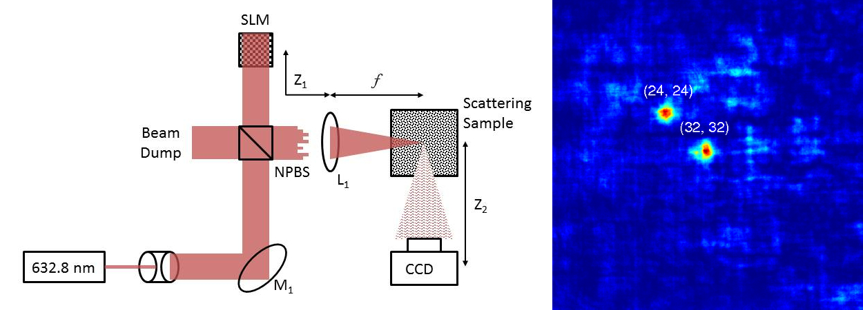
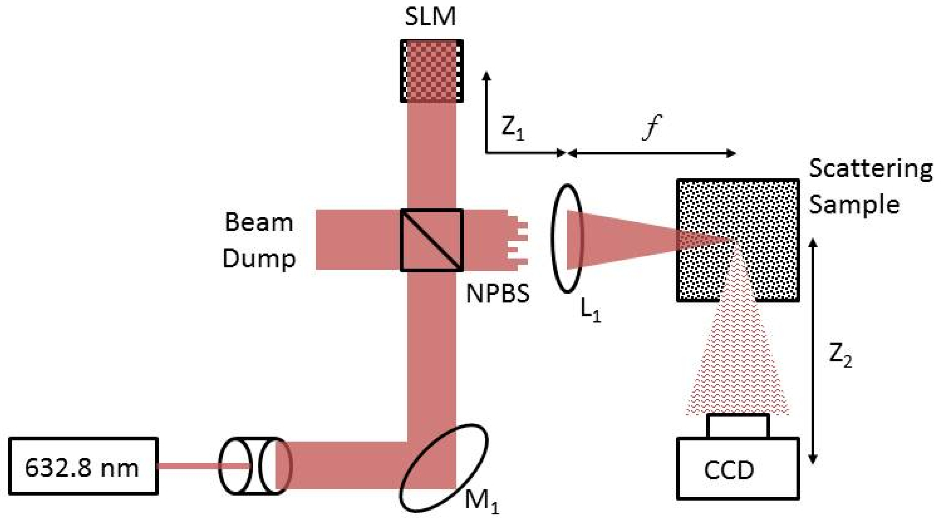
The RM of each sample was measured in three separate locations using the optical setup shown in Figure 1. This is the same optical setup used in the original reflective inverse diffusion experiments where the rough-surface reflector was placed at the focus of lens [7]. The RM measurements were also repeated using the optical setup shown in Figure 2, where the single lens system produces a -scale image of the SLM on the rough-surface reflector. The RM was then used to refocus light individually to each of the M segments of the observation plane. The average and maximum intensity enhancement for each sample is shown in Table 1.
3.2. Simulations
The propagation model assumes that the SLM is illuminated by a unit amplitude ideal plane wave. The individual SLM segments are represented by unimodular complex coefficients. The phase of these coefficients represents the phase delay imparted by the SLM segments onto the incident plane wave. At nm, aluminum has a reflectivity greater than , and a complex index of refraction of with a penetration depth of just a few nanometers [18,19]. Thus, absorption and transmission are neglected when modeling the aluminum rough-surface reflectors and the samples are modeled as unimodular complex numbers. The random phase imparted by the rough surface is related to the surface-height fluctuations or surface roughness. Assuming a Gaussian surface-height distribution with a standard deviation equal to or greater than , the phase distribution becomes uniform when wrapped to the interval [15].
Diffraction-based models were simulated using the MATLAB® two-dimensional FFT (fast Fourier transform) and the Rayleigh–Sommerfeld transfer function [20]. For the focal-plane optical setup in Figure 1, the complex field at the observation plane is calculated using the Rayleigh–Sommerfeld transfer function and spatial Fourier transform property of the lens. The field in the observation plane is then given by [7],
where k is the wavenumber, and is the Rayleigh–Sommerfeld transfer function [21]. The coordinate axes of source plane at the SLM are given in , where the coordinate axes of the sample plane at the lens focus are given in . The horizontal and vertical spatial frequencies of the source and sample planes are and , respectively. The focal length of lens is f, and and are the distances from the SLM to the lens and the reflective sample to the CCD, respectively. The rough surface is represented by , where the phase function is a random uniform distribution from .
Ideal imaging is assumed for the configuration in Figure 2. Propagation from the SLM to the rough sample is reduced to a global phase shift and can be ignored. The rough surface then randomizes the phase of the ideal image, which is then propagated to the CCD in the observation plane using the Rayleigh–Sommerfeld transfer function. Thus, the field in the observation plane is given by,
where is the object distance from the SLM to the lens , and is the image distance from the lens to the rough-surface sample.
3.3. Segment Size
The number of SLM segments, N, is directly proportional to the maximum ideal enhancement of the refocused spot on the CCD. The parallel wavefront modulation method used to measure the RM requires intensity measurements [17]. For all the experimental RM measurements, the SLM was divided into 1024 equal-sized segments, arranged , which required 4104 intensity measurements to measure the RM. This was the largest number of segments that could be equally sized and utilized the entire SLM area.
The segment size of the CCD also affects enhancement. Parallel wavefront modulation measures the RM in two separate halves. If the CCD segment size is too large, the two halves of the RM may focus on separate locations within the same CCD segment, resulting in a larger blurred spot with lower overall enhancement. The only indication that a CCD segment is too large is the lack of enhancement increase during the third step of parallel wavefront optimization of phase matching the two halves of the RM. Selecting a CCD segment size that is smaller than necessary increases the total number of segments and increases the memory and processing time of the RM measurement. The best CCD segment size was found to be approximately the size of the predicted diffraction-limited spot of the optical system.
The predicted spot size for the optical system shown in Figure 1 was calculated in the original reflective inverse diffusion proof-of-concept experiments [7]. The radius of the final spot was given by
where is the distance from the sample to the CCD, f is the focal length of lens , is the width of the SLM, and N is the total number of SLM segments. Using Equation (7), the CCD segment size for the focal-plane optical setup is 120 m, which is pixels on the Thorlabs 40740M CCD.
The predicted spot size for the imaging system in Figure 2 is calculated as the diffraction-limited spot produced by an aperture the size of the demagnified SLM image that is applied to the rough-surface reflector. The radius of the final spot is then given by,
where is the object distance from the SLM to lens , and is the image distance from lens to the rough-surface sample. Thus, the segment size for the imaging system is 317 m, which is pixels on the Thorlabs 4070M CCD.
4. Results and Analysis
4.1. Experiments
The RM was measured three times along the diagonal of each sample, top left corner, center, and bottom right corner, for both the focal-plane and imaging optical systems. The RM was then used to focus the incident beam to 1024 different segments of the CCD and record the enhancement of the target segment over the background segments. The maximum enhancement for each sample, , is the average peak enhancement from each of the three measured RMs. The average enhancement for each sample, , is the mean enhancement value over all the segments from all three RM. The and for each of the five samples are recorded in Table 1.
Data trends in Figure 3 show that enhancement decreases as surface roughness increases for the imaging system. The enhancement for the focal-plane system is almost flat with the average enhancement just slightly larger than 1; the target segment intensity is not significantly higher than the background. The difference between constructive and destructive interference is a surface height change of , thus the rate at which the surface height changes is a better predictor for enhancement. The RMS surface slope indicates the rate of the surface-height fluctuations and was determined from the profile data from each sample. For discrete profile data, the surface slope is given by [22],
where K is the total number of measurements, is the surface height from the profilometer, is the lateral sample distance, and , the average slope. The RMS slopes of the samples are included in Table 1. In general, the samples with larger RMS slope showed lower enhancement.
The correlation length, in Table 1, is defined as the shift required to lower the autocorrelation of the surface height profile by a factor of of the maximum value [22]. The apparent inverse relationship between correlation length and enhancement is counter-intuitive but is not conclusive since the samples with the longest correlation length also have the highest roughness. None of the samples showed Gaussian surface-height distributions, and with regards to reflective inverse diffusion, the standard definition used for correlation length is overly optimistic due to the small surface-height difference between constructive and destructive interference. For reflective inverse diffusion, the proposed lateral dimension, in Table 1, is described as the distance required to achieve a change in surface height given the RMS slope. The slope is calculated for each profile measurement recorded by the stylus profiler and averaged to produce a single for each sample. The surface profiles collected from the bead blasted sample showed widely varying slopes up to from the average slope used to determine . The enhancement performance from the bead blasted sample is likely inflated by an RM measured in area of the sample with a significantly larger than calculated from the average slope. Enhancement is plotted with in Figure 4. The imaging system shows that enhancement increases with . The data is inconclusive in the focal-plane system due to low enhancement values and virtually flat trends.
4.2. Simulations
The RM produced by the simulation of the focal-plane system in Figure 1 was used to calculate the enhancement for 1024 different observation plane segments. The rough-surface reflector was made up of individual segments with a uniform phase distribution. The phase of each segment was independent, which leads to a delta-correlated sample. The segment size is a measure of lateral correlation, but due to the phase independence between each segment, it was not directly comparable to of the tested aluminum samples.
The phase of the simulated rough-surface segments is a uniform distribution over []. If bounded over a single wavelength, the phase distribution gives a surface height range from [. Since the simulated rough-surface segments are independent, the surface-height difference () in Equation (9) for surface slope is a random variable with the same uniform distribution and an expected value of . Assuming a mean slope of , the RMS surface slope for the simulated rough surface is given by,
where is the dimension of the simulated rough-surface sample segment. For the simulations , the simulated rough-surface segment size.
Lateral surface dimensions () from 10.3 m to 660 m were simulated. Maximum enhancement was achieved with 41 m , which produced an enhancement of or 88% of the predicted ideal maximum from Equation (3). The best average enhancement of the 1024 simulated measurements was achieved with 82 m, which produced an enhancement of . Increasing beyond 82 m caused both the maximum and average enhancement to decrease.
In the focal-plane system, the individual SLM segments act as individual apertures. The spacing and phase of the SLM segments create fringe patterns in the diffraction-limited spot incident on the rough-surface reflector. The sum of all interferences from the SLM segment pairs produces a wavefront that conjugates the phase imparted by the rough-surface reflector to produce a wave that converges in the observation plane. Segment pairs that are farthest apart produce the narrowest fringe spacing of 41 m. This represents the smallest lateral surface dimension () that the focal-plane system can conjugate and explains the peak maximum enhancement at 41 m for the focal-plane system, see Figure 5. Using the RM to refocus light ensures that the light at the target segment is all in-phase, but it does not guarantee it is the only segment where the light is in-phase. In the focal-plane system, as the correlation length of the simulated sample increased, higher-order fringes are incident on the same simulated sample segment and remain in phase. This produces additional foci in the observation plane that increase background intensity and decrease enhancement as the correlation length is increased (see Figure 5).
Simulations of the imaging system shown in Figure 2 assumed a 1- ideal image of the SLM projected onto the rough-surface reflector. The SLM was modeled with n = 1024 equal-sized segments, arranged 32 × 32 across the SLM, each with an area of 31.25 m × 31.25 m. The lateral surface dimension of the simulated SLM image is the dimension of a single SLM segment, m. The rough-surface reflector was modeled with discrete segments all with unit magnitude and a uniform phase distribution. The of the simulated rough surface was adjusted by varying the number of segments used in the model. Simulations were performed with rough-surface lateral dimensions () as high as 500 m, and as low as 7.8 m.
When the lateral surface dimension of the simulated rough surface was identical to the lateral surface dimension of SLM image, , the simulated RM achieved a maximum enhancement of with an average enhancement of . This represents 30–65% of the performance predicted by Equation (3). This performance drops to 28–39% as the correlation length of the rough surface decreases to of the correlation length of SLM image. The best performance of 40–73% was achieved when .
The simulations with the longer lateral surface dimension () produced greater enhancement, both the maximum achieved by a single observation plane segment and the average enhancement of the simulated 1024 observation-plane segments. The enhancement is plotted with lateral surface dimension () for both the focal-plane and imaging systems in Figure 5. The focal-plane system achieves much higher peak enhancement, but only at specific correlation lengths before it rapidly decreases. The imaging system outperforms the focal-plane system at shorter values of in both maximum and average enhancement. For longer values of , the enhancement of the imaging system remains stable and does not decrease.
In the imaging case, the SLM is imaged and directly applied to the rough-surface reflector. The SLM segments conjugate the phase changes imparted by the reflector and produce a converging wavefront. As the lateral surface dimension () of the sample increases, fewer adjustments to the phase map are required. Extended to the perfect mirror case, the SLM phase map becomes the discretized phase function for a positive lens with the focal length in the observation plane. The background intensity does not increase with correlation length as in the focal-plane system. As correlation length increases, diffraction from the SLM segments and phase quantization error of the SLM become the limiting factors for enhancement.
4.3. RM Properties
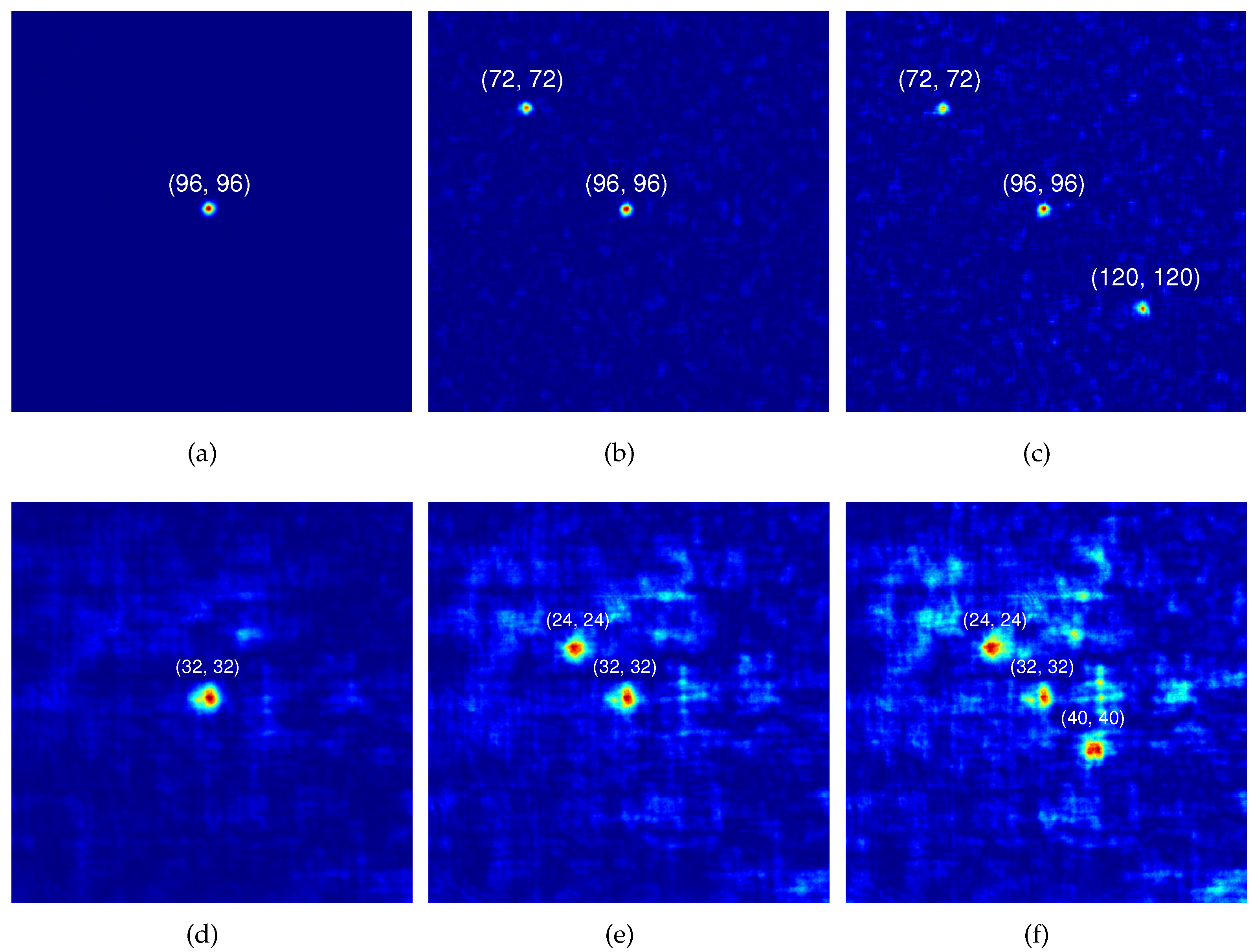
The RM measured with the focal-plane and imaging systems both maintained the ability to refocus light to a single CCD segment or multiple segments simultaneously, similar to their transmission matrix counterparts. Multiple segments are enhanced simultaneously using the same process as the transmission case, by using a linear combination of the rows of the RM [17]. Simulations of the focal-plane system show single-segment enhancement in Figure 6a, and multi-segment enhancements in Figure 6b,c. The imaging system with the 600-grit aluminum sample demonstrates single-segment and simultaneous multi-segment enhancements and are shown in Figure 6d–f. Each spot location is labeled with its corresponding (row, column) coordinates. As the enhancement was split over multiple segments, the background intensity becomes more visible.
4.4. Predicted vs. Measured Enhancement
The best enhancement values from the aluminum samples were 10 to 24 times the RMS background intensity, which is less than 10% of the average enhancement of 300 to 400 achieved in simulation. Device error does not account for this discrepancy. Simulations included a random intensity fluctuation of for each CCD pixel, while SLM pixels included a similar fluctuation in phase. For both the imaging and focal-plane simulations, this random device error of only decreased the average enhancement by approximately 10%. The RM is measured using the temporal FFT of intensity measurements from the CCD. Since the random intensity fluctuations do not occur at a specific frequency, the noise does not have a significant effect on the RM coefficients.
The aluminum samples are assumed to be stable for much longer than the five minutes it takes to measure the RM. However, mechanical sources in the laboratory, such as the ventilation system, fume hoods, cooling fans, water and compressed air lines, produce micro-vibrations in the optical setup that cause the incident light to shift on the rough-surface reflector. The oscillation of the RM measurement area produces intensity measurements that belong to several different RMs. For the imaging system with a simulated rough-surface lateral dimension of 7.8 m, incorporating a random vertical and horizontal shift of the sample by 23.4 m, reduces average enhancement to and maximum enhancement to . For the focal-plane system with a simulated rough-surface lateral dimension of 10.3 m, a simulated vibration magnitude of 20.6 m produces maximum enhancement of and an average enhancement of .
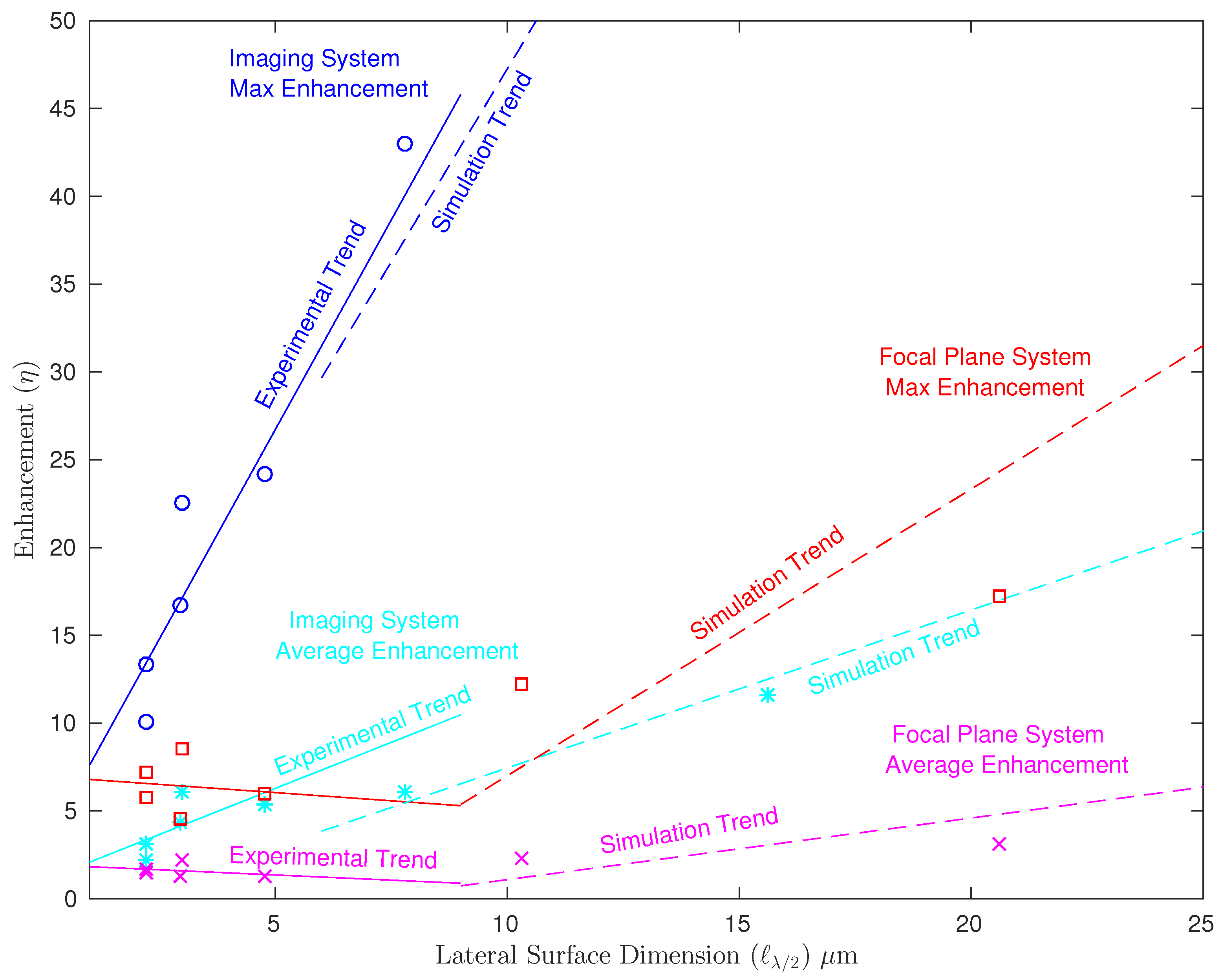
The lateral surface dimension () for the aluminum samples is much smaller than can be simulated without an unacceptable increase in processing time. However, trends between enhancement and from the experiments and simulations were extended and plotted for comparison in Figure 7. The imaging system shows the best alignment between experimental and simulation trends for maximum enhancement. The imaging system average enhancement trend lines for experimental and simulation data have matching slope despite the increase in separation. The experimental data for the focal-plane system showed very low enhancement with predominately flat trends for both average and maximum measured enhancement. Similar enhancement levels are achieved in simulation for 10.3 m with the addition of the random vibration oscillation of 20.6 m. Simulations show enhancement increases for 10.3 m. This could indicate that the correlation length of the aluminum samples is too small for the focal-plane system to be effective in the given laboratory conditions.
5. Conclusions
Yoon’s method for measuring transmission matrices was successfully implemented to measure an RM. The method only requires the optical system to be linear. Both the focal-plane and the imaging systems produced RM capable of refocusing light onto the CCD. The RM is capable of enhancing a single CCD segment, or multiple segments simultaneously. For single segment enhancement, the focal plane system achieved a maximum intensity enhancement of 8.5 and the imaging system achieved a maximum intensity enhancement of 24.2.
Simulations showed that the focal-plane system achieves higher levels of enhancement for specific lateral surface dimensions (); outside of this optimum range, the imaging system produces better enhancement. Laboratory data showed that the imaging system consistently produced higher levels of enhancement than the focal-plane system on all of the samples tested. This was expected as simulations predicted the imaging system would achieve higher levels of enhancement at lower values of .
The enhancement for both the focal-plane and imaging systems was significantly lower than that predicted by Equation (3) for the ideal simulated results. The primary cause of this was minute mechanical vibrations in the optical setup. This problem is accentuated due to the much longer propagation distances associated with reflective inverse diffusion and are not found in the transmissive case. Although enhancement for both methods was affected, incorporating a simple random vibration in the simulation model showed that the imaging system was capable of greater enhancement values in this non-ideal case. This is corroborated by the higher enhancement values achieved by the imaging system in the laboratory.
Further research is required to solidify the RM measurement method. Improving the vibration isolation of the optical system will be key to improving the RM enhancement performance. Mathematical methods for combating the effects of vibration, such as DDDAS [23], should also be explored as a more cost-effective solution. Ideally, in the imaging case, the incident light is scattered by the same part of the rough surface regardless of which CCD segment is enhanced. Since the rough surface is assumed to be static, the scattering is deterministic [4]. Further research may yield methods of exploiting the deterministic process and lead to methods of reconstructing missing portions of the RM from partial data, or expanding an RM to include additional CCD segment locations without requiring the RM to be re-measured.
Acknowledgments
This work is supported by the Air Force Office of Scientific Research. The views expressed in this article are those of the authors and do not reflect the official policy or position of the United States Air Force, Department of Defense, or the United States Government. This material is declared a work of the U.S. Government and is not subject to copyright protection in the United States.
Author Contributions
Kenneth Burgi developed the mathematical model, conducted the MATLAB® simulations, laboratory experiments, and wrote the paper. Michael Marciniak contributed to the idea, the mathematical model, and organization of the research. Mark Oxley contributed to development of the mathematical model. Stephen Nauyoks supplied laboratory test samples and assisted with the interpretation of the experimental results.
Conflicts of Interest
The authors declare no conflict of interest.
Abbreviations
The following abbreviations are used in this manuscript:
| AFIT | Air Force Institute of Technology |
| DMD | digital mirror device |
| LCoS | liquid crystal on silicon |
| SLM | spatial light modulator |
| HeNe | helium-neon |
| CCD | charge-coupled device |
| NPBS | non-polarizing beam splitter |
| BNS | Boulder Nonlinear Systems |
| DFT | discrete Fourier transform |
| FFT | fast Fourier transform |
| TM | transmission matrix |
| RM | reflection matrix |
| DMD | digital micro-mirror device |
| SBIG | Santa Barbara Instruments Group |
| BRDF | Bidirectional Reflectance Distribution Function |
| FWHM | full width at half max |
| RMS | root mean square |
| SNR | signal-to-noise ratio |
| SF | spatial filter |
| NPBS | non-polarizing beam splitter |
| DDDAS | dynamic data driven applications systems |
References
- Freund, I. Looking through walls and around corners. Phys. A Stat. Mech. Appl. 1990, 168, 49–65. [Google Scholar] [CrossRef]
- Aulbach, J.; Gjonaj, B.; Johnson, P.M.; Mosk, A.P.; Lagendijk, A. Control of light transmission through opaque scattering media in space and time. Phy. Rev. Lett. 2011, 106, 103901. [Google Scholar] [CrossRef] [PubMed]
- Cui, M. A high speed wavefront determination method based on spatial frequency modulations for focusing light through random scattering media. Opt. Express 2011, 19, 2989–2995. [Google Scholar] [CrossRef] [PubMed]
- Vellekoop, I.; Mosk, A. Focusing of light by random scattering. arXiv, 2006; arXiv:cond-mat/0604253. [Google Scholar]
- Vellekoop, I.M.; Mosk, A. Focusing coherent light through opaque strongly scattering media. Opt. Lett. 2007, 32, 2309–2311. [Google Scholar] [CrossRef] [PubMed]
- Vellekoop, I.; Mosk, A. Phase control algorithms for focusing light through turbid media. Opt. Commun. 2008, 281, 3071–3080. [Google Scholar] [CrossRef]
- Burgi, K.; Ullom, J.; Marciniak, M.; Oxley, M. Reflective Inverse Diffusion. Appl. Sci. 2016, 6, 370. [Google Scholar] [CrossRef]
- Popoff, S.; Lerosey, G.; Carminati, R.; Fink, M.; Boccara, A.; Gigan, S. Measuring the transmission matrix in optics: An approach to the study and control of light propagation in disordered media. Phys. Rev. Lett. 2010, 104, 100601. [Google Scholar] [CrossRef] [PubMed]
- Popoff, S.; Lerosey, G.; Fink, M.; Boccara, A.C.; Gigan, S. Controlling light through optical disordered media: Transmission matrix approach. New J. Phys. 2011, 13, 123021. [Google Scholar] [CrossRef]
- Conkey, D.B.; Caravaca-Aguirre, A.M.; Piestun, R. High-speed scattering medium characterization with application to focusing light through turbid media. Opt. Express 2012, 20, 1733–1740. [Google Scholar] [CrossRef] [PubMed]
- Drémeau, A.; Liutkus, A.; Martina, D.; Katz, O.; Schülke, C.; Krzakala, F.; Gigan, S.; Daudet, L. Reference-less measurement of the transmission matrix of a highly scattering material using a DMD and phase retrieval techniques. Opt. Express 2015, 23, 11898–11911. [Google Scholar] [CrossRef] [PubMed]
- Yılmaz, H.; Vos, W.L.; Mosk, A.P. Optimal control of light propagation through multiple-scattering media in the presence of noise. Biomed. Opt. Express 2013, 4, 1759–1768. [Google Scholar] [CrossRef] [PubMed]
- Katz, O.; Small, E.; Silberberg, Y. Looking around corners and through thin turbid layers in real time with scattered incoherent light. Nat. Photonics 2012, 6, 549–553. [Google Scholar] [CrossRef]
- Sen, P.; Chen, B.; Garg, G.; Marschner, S.R.; Horowitz, M.; Levoy, M.; Lensch, H. Dual photography. ACM Trans. Gr. (TOG) 2005, 24, 745–755. [Google Scholar] [CrossRef]
- Goodman, J.W. Speckle Phenomena in Optics: Theory and Applications; Roberts and Company Publishers: Englewood, CO, USA, 2007. [Google Scholar]
- Williams, M.W. Depolarization and cross polarization in ellipsometry of rough surfaces. Appl. Opt. 1986, 25, 3616–3622. [Google Scholar] [CrossRef] [PubMed]
- Yoon, J.; Lee, K.; Park, J.; Park, Y. Measuring optical transmission matrices by wavefront shaping. Opt. Express 2015, 23, 10158–10167. [Google Scholar] [CrossRef] [PubMed]
- Rakić, A.D. Algorithm for the determination of intrinsic optical constants of metal films: Application to aluminum. Appl. Opt. 1995, 34, 4755–4767. [Google Scholar] [CrossRef] [PubMed]
- Smith, D.; Shiles, E.; Inokuti, M. The optical properties of metallic aluminum. Handb. Opt. Constants Solids 1985, 1, 369–406. [Google Scholar]
- Voelz, D.G. Computational Fourier Optics: A MATLAB Tutorial; Spie Press Bellingham: Bellingham, WA, USA, 2011. [Google Scholar]
- Goodman, J.W. Introduction to Fourier Optics; Roberts and Company Publishers: Englewood, CO, USA, 2005. [Google Scholar]
- Stover, J.C. Optical Scattering: Measurement and Analysis; SPIE Optical Engineering Press: Bellingham, WA, USA, 1995; Volume 2. [Google Scholar]
- Darema, F. Dynamic data driven applications systems: New capabilities for application simulations and measurements. In Computational Science–ICCS, Proceedings of International Conference on Computational Science, Atlanta, GA, USA, 22–25 May 2005; Springer: Berlin, Germany, 2005; pp. 610–615. [Google Scholar]
Figure 1.
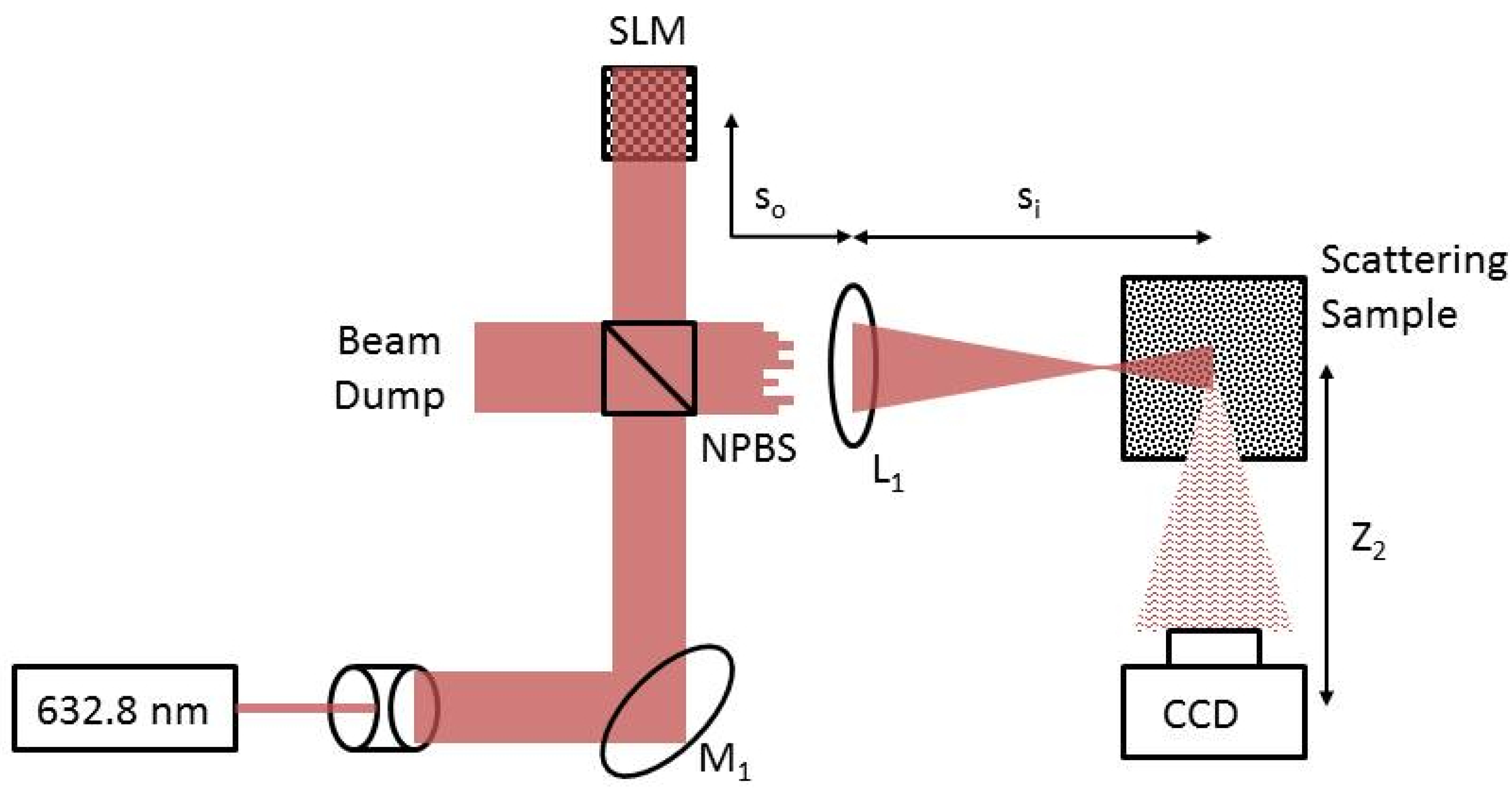
Focal-plane optical setup for reflective inverse diffusion. A vertically polarized HeNe laser is expanded, collimated, and normally incident on the SLM (spatial light modulator). The phase modulated beam is then focused onto the rough-surface reflector with positive lens () and the reflected speckle pattern is recorded by the CCD (charged-coupled device). The mirror () and the NPBS (non-polarizing beam splitter) are used to allow normal incidence with the SLM. For focal-plane experiments and simulations, the lens focal length, f, is 500 mm, and the distances and are cm and cm, respectively.
Figure 1.
Focal-plane optical setup for reflective inverse diffusion. A vertically polarized HeNe laser is expanded, collimated, and normally incident on the SLM (spatial light modulator). The phase modulated beam is then focused onto the rough-surface reflector with positive lens () and the reflected speckle pattern is recorded by the CCD (charged-coupled device). The mirror () and the NPBS (non-polarizing beam splitter) are used to allow normal incidence with the SLM. For focal-plane experiments and simulations, the lens focal length, f, is 500 mm, and the distances and are cm and cm, respectively.

Figure 2.
Image plane optical setup for reflective inverse diffusion. A vertically polarized HeNe laser is expanded, collimated, and normally incident on the SLM. The lens () produces a demagnified image of the phase modulated beam onto the rough-surface reflector and the reflected speckle pattern is recorded by the CCD. The mirror () and the NPBS are used to allow normal incidence with the SLM. The demagnification of the system is .

Figure 3.
Enhancement () vs. Surface Roughness (). The surface roughness measured by the Tencor profilometer is plotted with enhancement. Linear trend lines are included. For the focal-plane system, maximum enhancement is shown in red, while average enhancement is shown in magenta. For the imaging system, maximum enhancement is shown in blue, while average enhancement is shown in cyan.
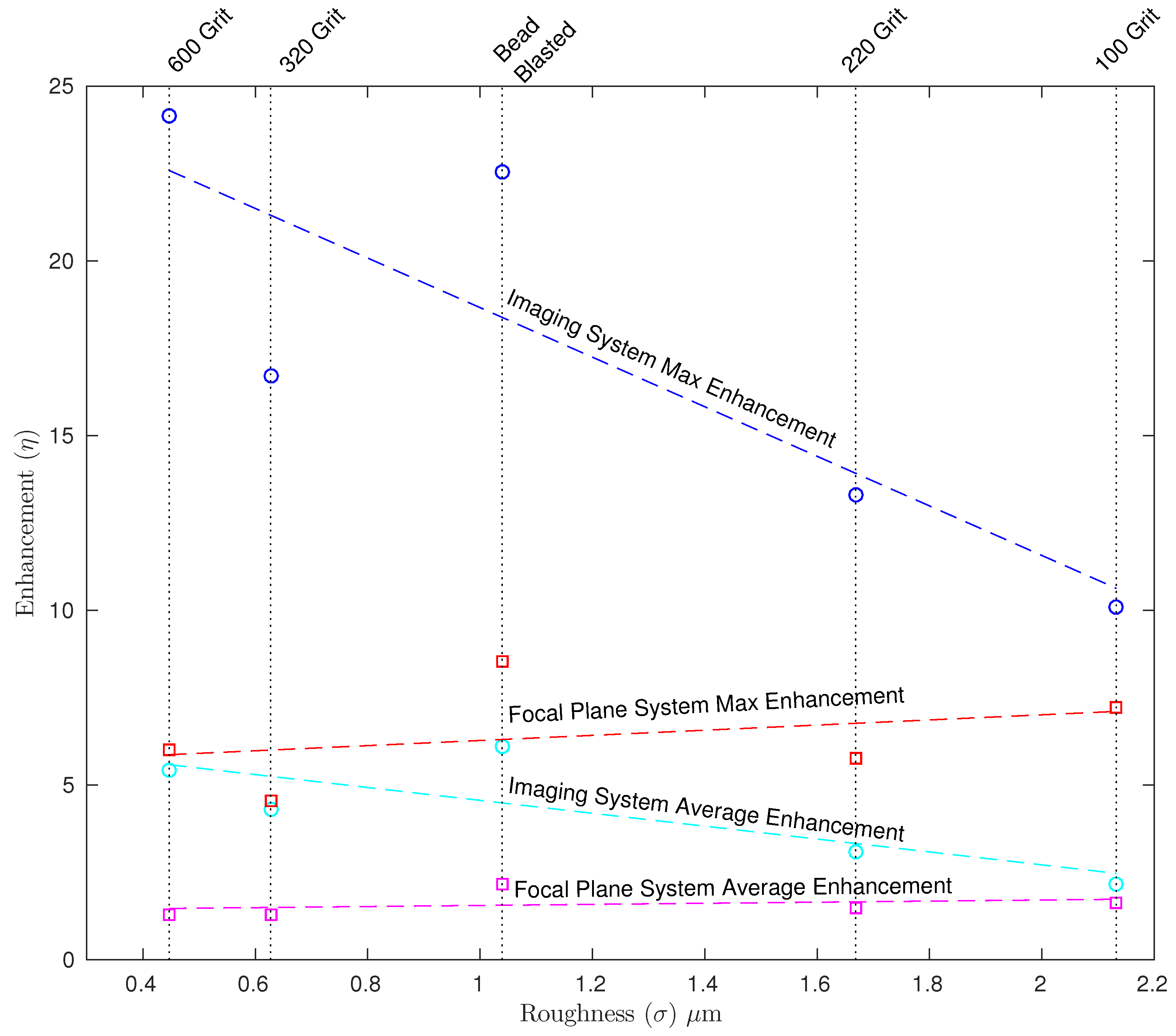
Figure 4.
Enhancement () vs. Lateral surface dimension (). The lateral surface dimension, , is plotted with enhancement. The focal-plane system shows no change in enhancement with . However, the average enhancement of 1 indicates that the target segment has the same intensity as the background.
Figure 4.
Enhancement () vs. Lateral surface dimension (). The lateral surface dimension, , is plotted with enhancement. The focal-plane system shows no change in enhancement with . However, the average enhancement of 1 indicates that the target segment has the same intensity as the background.

Figure 5.
Simulated Enhancement () vs. Lateral Surface Dimension (). The red solid line shows average enhancement of the focal-plane system, while the red dotted line shows maximum enhancement. The solid blue line shows average enhancement of the imaging system, while the blue dotted line represents maximum enhancement.
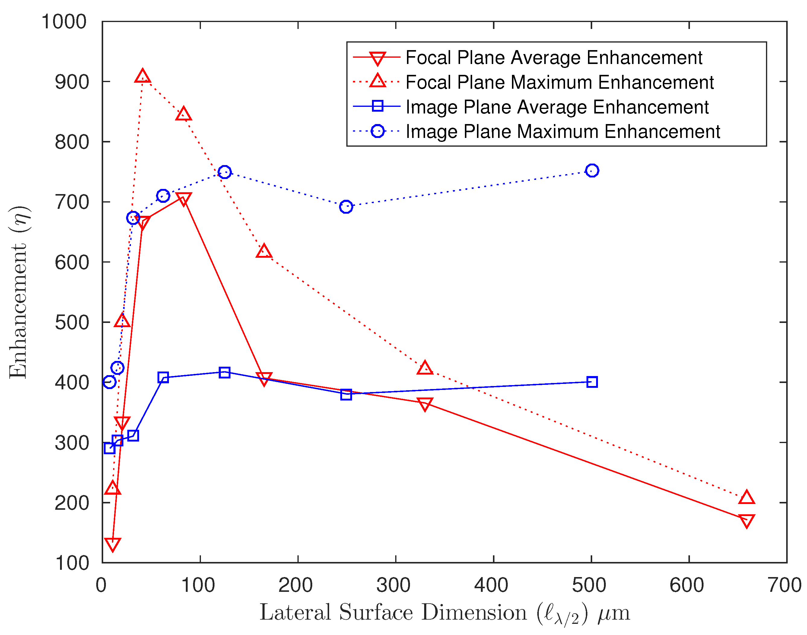
Figure 6.
Observation plane intensity patterns (a–c) are computer simulations of the focal-plane system and (d–e) are laboratory results of the imaging system with the 600 grit aluminum sample. Above each spot are the (row, column) coordinates of the given observation plane segment. Phase maps generated by the RM (reflection matrix) are used to refocus light to single or multiple segments in the observation plane. (a) a simulated single-segment enhancement of over background speckle; (b) simulation of two foci optimized simultaneously at and with enhancements of and 56, respectively; (c) simulation of three foci generated with increased background speckle at , , and with enhancement values of , 32, and 29, respectively; (d) demonstrated single-segment enhancement of over background speckle using the imaging system with the 600 grit aluminum sample (e) two segments are optimized simultaneously, measured enhancement for both foci is ; (f) three foci are generated with increased background speckle at , , and , enhancement values are , 6, and 7, respectively.

Figure 7.
Enhancement () vs. Lateral Surface Dimension (). Simulations are conducted with a random shift in the sample prior to each intensity measurement. The solid lines are experimental data trends, and dashed lines represent simulation data trends. The simulated focal-plane system is subject to a random 20.6-m shift; maximum enhancement is shown in red, while average enhancement is shown in magenta. The simulated imaging system is subject to a random 23.4-m shift; maximum enhancement is shown in blue, while average enhancement is shown in cyan.


Table 1.
Summary table for the five aluminum samples. Roughness () is the standard deviation of the sample surface height. Correlation () is the autocorrelation shift to reduce the maximum value by . Slope (s) is the RMS (root mean square) surface slope. Correlation () is the lateral distance required to change the surface height by at the RMS slope (s). The samples average enhancement () and maximum enhancement () achieved with each optical setup is included.
| Aluminum | Roughness | Correlation | Slope | Correlation | Focal-Plane | Image Plane | ||
|---|---|---|---|---|---|---|---|---|
| Samples | /m | /m | s | /m | ||||
| 100 Grit | 2.13 | 54.25 | 0.143 | 2.21 | 1.6 | 7.2 | 2.2 | 10.1 |
| 220 Grit | 1.67 | 35.25 | 0.141 | 2.24 | 1.5 | 5.8 | 3.1 | 13.3 |
| Bead Blasted | 1.04 | 30.25 | 0.105 | 3.00 | 2.2 | 8.5 | 6.1 | 22.5 |
| 320 Grit | 0.63 | 13.75 | 0.107 | 2.97 | 1.3 | 4.5 | 4.3 | 16.7 |
| 600 Grit | 0.45 | 16.00 | 0.066 | 4.79 | 1.3 | 6.0 | 5.4 | 24.2 |
© 2017 by the authors. Licensee MDPI, Basel, Switzerland. This article is an open access article distributed under the terms and conditions of the Creative Commons Attribution (CC BY) license (http://creativecommons.org/licenses/by/4.0/).
Share and Cite
MDPI and ACS Style
Burgi, K.; Marciniak, M.; Oxley, M.; Nauyoks, S. Measuring the Reflection Matrix of a Rough Surface. Appl. Sci. 2017, 7, 568. https://doi.org/10.3390/app7060568
AMA Style
Burgi K, Marciniak M, Oxley M, Nauyoks S. Measuring the Reflection Matrix of a Rough Surface. Applied Sciences. 2017; 7(6):568. https://doi.org/10.3390/app7060568
Chicago/Turabian StyleBurgi, Kenneth, Michael Marciniak, Mark Oxley, and Stephen Nauyoks. 2017. "Measuring the Reflection Matrix of a Rough Surface" Applied Sciences 7, no. 6: 568. https://doi.org/10.3390/app7060568
Note that from the first issue of 2016, this journal uses article numbers instead of page numbers. See further details here.