Construction of Compact Finite Difference Schemes by Classic Differential Quadrature

Abstract

Using classic differential quadrature formulae and uniform grids, this paper systematically constructs a variety of high-order finite difference schemes, and some of these schemes are consistent with the so-called boundary value methods. The derived difference schemes enjoy the same stability and accuracy properties with correspondent differential quadrature methods but have a simpler form of calculation; thus, they can be seen as a compact format of classic differential quadrature methods. Through systematic Fourier stability analysis, the characteristics such as the dissipation, dispersion and resolution of the different schemes were studied and compared.

1. Introduction

Many physical phenomena possess a range of space and time scales, and direct numerical simulations of these processes require all the relevant scales to be properly represented in the numerical model. These requirements have led to the development of the so-called compact finite difference scheme [1]. Usually, the compact schemes have much smaller numerical dispersion and dissipation errors than traditional finite difference schemes of the same order of accuracy on the same mesh. So far, researchers have developed a variety of compact difference schemes [2,3,4,5,6].

This paper presents a simple way for constructing the compact finite difference schemes by the use of the differential quadrature method (DQM). The DQM was firstly proposed by Bellman and Casti in the early 1970s [7,8]. The basic idea of DQM is to extend analogously the numerical integration rule to the numerical differentiation, where the derivative of a function on a coordinate direction is expressed as the weighted linear combination of function values for all discrete points along this direction.

At present, the differential quadrature method has been widely developed. According to the used trial or test function, the differential quadrature method generally includes the classical differential quadrature method, harmonic differential quadrature method, Fourier differential quadrature method, and so on. The classic differential quadrature method mainly uses the general polynomial or Lagrangian interpolation function as a test function, the harmonic differential quadrature method uses the trigonometric function as the trial function, while the Fourier differential quadrature method uses Fourier series expansion as the trial function [9,10]. Theoretically, the above differential quadrature rules can be used either for spatial discretization or for time discretization. In other words, the differential quadrature method can be used for the solution of both the partial differential equation and the ordinary differential initial problem [11,12,13,14,15]. In summary, differential quadrature methods have the advantages of high precision, good numerical stability and convenient programming, and have been successfully applied in many fields [16,17].

Using classic differential quadrature formulae and uniform grids, we systematically constructed a variety of finite difference schemes, and some of these schemes are consistent with the boundary value methods (BVM) proposed by Brugnano et al. [18,19]. Considering that the derived difference schemes enjoy the same stability and accuracy properties with correspondent DQM but have a simpler form of calculation, the derived difference schemes can be regarded as the compact expression of classic DQM. Naturally, these compact difference methods could be used instead of classic differential quadrature methods for engineering applications [20].

2. The Classic Differential Quadrature Methods

Suppose function $f\left(x\right)$ is sufficiently smooth in the considered interval, and the first-order derivative of $f\left(x\right)$ at each grid point $c_p,p\in (1,s)$ is approximated by a linear sum of all the function values in the whole domain, that is

$${\frac{\partial f\left(x\right)}{\partial x}|}_{x=c_p}\equiv f^{\left(1\right)}(c_p)={\displaystyle \sum _{q=0}^s{g}_{pq}f\left(c_q\right)}$$

(1)

The above Equation (1) is simply the basic expression of DQM, within which $g_{pq}$ represents the weighting coefficient of DQM; s is the grid number of the partition of each interval; and $c_p,p\in (0,s)$ represent the grid points.

The weighting coefficients of DQM only depend on the trial function and the discrete sample points, namely, the distribution of grid points, and have nothing to do with a specific problem. Usually, we would like to choose the general polynomial or Lagrange interpolation polynomial as the trial function, and use these functions to approximate the value of $f^{\left(1\right)}\left(x\right)$ at each grid points, which is defined as the classic DQM in this paper. The researchers have proved that the weighting coefficients derived by these two trial functions are consistent [17]. The concrete calculation expression of weighting coefficients for classic DQM can be described as follows:

$$\{\begin{array}{l}{g}_{pq}=\frac{M^{\left(1\right)}\left(c_p\right)}{(c_p-c_q)M^{\left(1\right)}\left(c_q\right)},p\ne q\\ g_{pp}=-{\displaystyle \sum _{q=1;q\ne p}^s{g}_{pq}}\end{array},p,q\in (0,s)$$

(2)

where,

$$M^{\left(1\right)}(c_z)\equiv {\displaystyle \prod _{q=1;q\ne z}^s(c_z-c_q)},z\in (0,s)$$

(3)

Obviously, if the distribution of grid points is centro-symmetric in the normalized interval $[0,1]$, it can be deduced that

$$c_{s-z}=1-c_z,M^{\left(1\right)}(c_{s-z})=-M^{\left(1\right)}(c_z),z\in (0,s)$$

(4)

$$g_{s-p,s-q}=-g_{pq},p,q\in (0,s)$$

(5)

Defining

$$\mathit{G}=\left(g_{pq}\right)\in R^{(s+1)\times (s+1)},p,q\in (0,s)$$

(6)

it can be known from Equation (5) that the weighting coefficient matrix $\mathit{G}$ is centro-antisymmetric.

Regarding the selection of grid points, there are some commonly used approaches, including the uniform grids, Chebyshev grids, Chebyshev-Gauss-Lobatto grids, and Legendre grids. These types of grids can be concretely described as follows.

• The uniform grids

  $$c_z=\frac{z}{s},z\in (0,s)$$

  (7)
• The Chebyshev grids

  $$c_0=0;c_z=\frac{1}{2}\left(1-\cos \left(\frac{2z-1}{2s-2}\pi \right)\right),z\in (1,s-1);c_s=1$$

  (8)
• The Chebyshev-Gauss-Lobatto grids

  $$c_z=\frac{1}{2}\left(1-\cos \left(\frac{z}{s}\pi \right)\right),z\in (0,s)$$

  (9)
• The Legendre grids
  $c_0=0$; $c_z,z\in (1,s)$ are the zero points of $\frac{d^s}{d{x}^s}\left(x^s{(x-1)}^{\mathrm{s}}\right)=0$; and $c_{s+1}=1$.

Take the following ordinary differentia initial value problem as an example

$$\{\begin{array}{l}\frac{d}{dx}y\equiv \dot{y}=f(x,y)\hfill \\ y(x=0)=y_0\hfill \end{array}$$

(10)

Supposing $x_n$ and $x_{n+1}$ represent respectively the starting point and ending point of an arbitrary interval, $h=x_{n+1}-x_n$ is the interval length or the so-called stencil length. Let $c=(x-x_n)/h$ and make the interval $x\in \left[x_n,x_{n+1}\right]$ normalized as $c\in \left[0,1\right]$, then the Equation (10) can be converted into

$$\frac{d}{dc}y=hf(x_n+ch,y(x_n+ch))$$

(11)

On this basis, we can apply the s-stage differential quadrature method (1) to Equation (11), and deduce that [15,16]

$$\tilde{\mathit{G}}\left[\begin{array}{c}{y}_{n+1}\\ ⋮\\ y_{n+s}\end{array}\right]+{\mathit{G}}_0{y}_n=h\left[\begin{array}{c}f({\tilde{x}}_1,y_{n+1})\\ ⋮\\ f({\tilde{x}}_s,y_{n+s})\end{array}\right]$$

(12)

in which $y_{n+z}=y(x_n+c_{z}h),z\in (0,s)$, ${\tilde{x}}_z=x_n+c_{z}h,z\in (1,s)$,

$$\tilde{\mathit{G}}=\left[\begin{array}{ccc}{g}_{11}& \cdots & g_{1s}\\ ⋮& \ddots & ⋮\\ g_{s1}& \cdots & g_{ss}\end{array}\right],{\mathit{G}}_0=\left[\begin{array}{c}{g}_{10}\\ ⋮\\ g_{s0}\end{array}\right]$$

(13)

If the initial value of $y_n$ is given, the value of state variable $y$ at different grid points, that is $y_{n+z}\in (1,s)$, can be obtained by solving the aforementioned nonlinear Equation (12).

It should be noted that, although the ordinary differential Equation (10) is used as a trial case, the variable $x$ in this equation can either represent the space or the time, and naturally the stencil length $h$ can be either a spatial discrete step size or a time discrete step. For ordinary differential initial value problems, it has been proven in reference [15] that, when using uniform grids, Chebyshev grids and Chebyshev-Gauss-Lobatto grids, the classical DQM—i.e., Equation (12)—are all s-stage s-order methods with A-stability, while the classic DQM combined with Legendre grids can achieve the accuracy of 2s-2 order.

3. Construction of Compact Difference Schemes by DQM

3.1. The Generalized Backward Differential Formulae

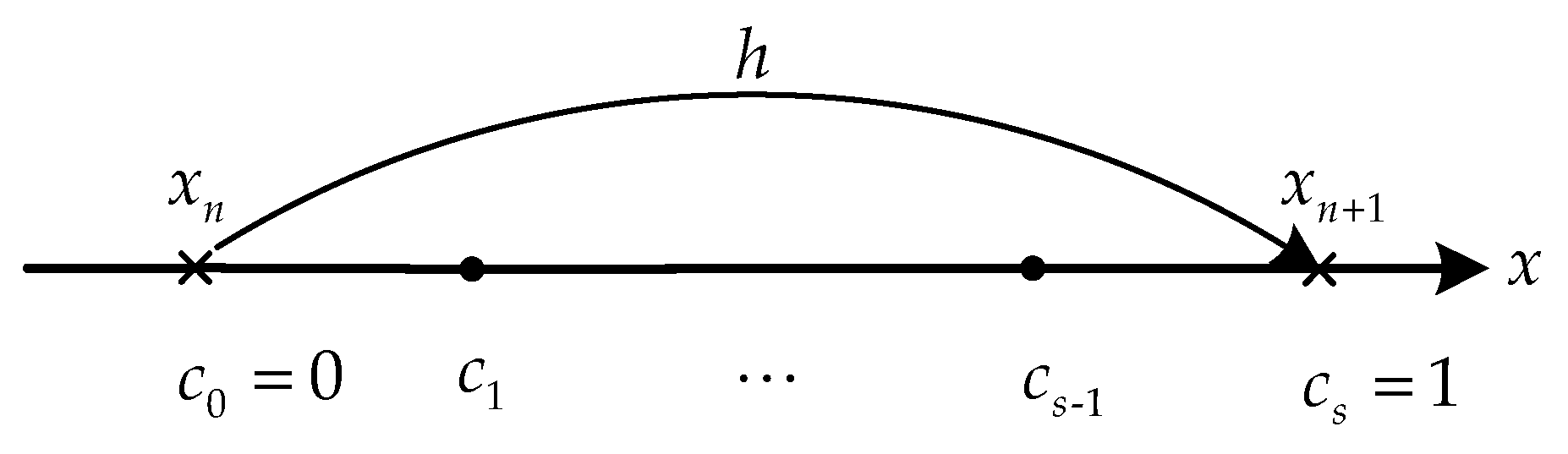
As shown in Figure 1, we divide the interval $x\in \left[x_n,x_{n+1}\right]$ into s segments, namely the grids, in which $h=x_{n+1}-x_n$, $x(x_n+c_{0}h)\equiv x_n$, $x(x_n+c_{s}h)\equiv x_{n+1}$.

Defining

$$\upsilon =\{\begin{array}{l}(s+2)/2,\mathrm{for}\mathrm{even}s\hfill \\ (s+1)/2,\mathrm{for}\mathrm{odd}s\hfill \end{array}$$

(14)

and taking the $\upsilon$-th equation from Equation (12), we can obtain

$$hf({\tilde{x}}_{\upsilon },y_{n+\upsilon })\equiv h{f}_{n+\upsilon }={\displaystyle \sum _{z=0}^s{\alpha }_z{y}_{n+z}}$$

(15)

in which,

$${\alpha }_z=g_{\upsilon z},z\in (0,s)$$

(16)

It can be shown that the above numerical method (15) has the accuracy of s-order.

The numerical method (15) has a similar form to the traditional backward difference formulae (BDF), but we will later show that this method has the better numerical stability then traditional BDF. Thus, for the sake of simplicity, we define this numerical method as the generalized backward difference formulae (GBDF).

When selecting the uniform grids, the coefficient values (${\alpha }_z$) of GBDF are shown in the following

Table 1. The coefficients of generalized backward difference formulae (GBDF) using uniform grids (for even s).

s	v	α0	α1	α2	α3	α4	α5	α6	α7	α8
$2$	$2$	$1$	$-4$	$3$
$4$	$3$	$-\frac{1}{3}$	$2$	$-6$	$\frac{10}{3}$	$1$
$6$	$4$	$\frac{1}{10}$	$-\frac{4}{5}$	$3$	$-8$	$\frac{7}{2}$	$\frac{12}{5}$	$-\frac{1}{5}$
$8$	$5$	$-\frac{1}{35}$	$\frac{2}{7}$	$-\frac{4}{3}$	$4$	$-10$	$\frac{18}{5}$	$4$	$-\frac{4}{7}$	$\frac{1}{21}$

and

Table 2. The coefficients of GBDF using uniform grids (for odd s).

s	v	α0	α1	α2	α3	α4	α5	α6	α7
$1$	$1$	$-1$	$1$
$3$	$2$	$\frac{1}{2}$	$-3$	$\frac{3}{2}$	$1$
$5$	$3$	$-\frac{1}{6}$	$\frac{5}{4}$	$-5$	$\frac{5}{3}$	$\frac{5}{2}$	$-\frac{1}{4}$
$7$	$4$	$\frac{1}{20}$	$-\frac{7}{15}$	$\frac{21}{10}$	$-7$	$\frac{7}{4}$	$\frac{21}{5}$	$-\frac{7}{10}$	$\frac{1}{15}$

.

For the uniform grids, we can define that

$$\overline{h}=(x_{n+1}-x_n)/s=h/s$$

(17)

therefore, the Equation (15) can be rewritten as the following formula

$$\overline{h}{f}_{n+\upsilon }={\displaystyle \sum _{z=0}^s\left(\frac{{\alpha }_z}{s}\right)y_{n+z}}$$

(18)

It can be verified from Table 1 and Table 2 that, the numerical method (18) is consistent with the GBDF proposed by Brugnano et al. [19]. In reference [21], it has been shown that the methods (18) are both A-stable numerical methods for time-domain numerical integration.

3.2. The Central Compact Difference Schemes

As is shown in Figure 1, let s be an even number. By defining

$$\upsilon =s/2$$

(19)

and selecting the $\upsilon$-th equation in Equation (12), it follows that

$$h{f}_{n+\upsilon }={\displaystyle \sum _{z=0}^s{\alpha }_z{y}_{n+z}}$$

(20)

in which,

$${\alpha }_z=g_{\upsilon z},z\in (0,s)$$

(21)

It can be shown that the above numerical method (20) has the accuracy of s-order. Furthermore, it can be verified that the coefficients ${\alpha }_z,z\in (0,s)$ are centro-antisymmetrical about ${\alpha }_{\upsilon }$. If the distribution of grid points is centro-symmetrical in the normalized interval $[0,1]$. So, the numerical method (20) can be called the central difference scheme.

When selecting the uniform grids, the coefficient values (${\alpha }_z$) of the method (20) are shown in the following

Table 3. The coefficients of central difference schemes using uniform grids.

s	v	α0	α1	α2	α3	α4	α5	α6	α7	α8
$2$	$1$	$-1$	$0$	$1$
$4$	$2$	$\frac{1}{3}$	$-\frac{8}{3}$	$0$	$\frac{8}{3}$	$-\frac{1}{3}$
$6$	$3$	$-\frac{1}{10}$	$\frac{9}{10}$	$-\frac{9}{2}$	$0$	$\frac{9}{2}$	$-\frac{9}{10}$	$\frac{1}{10}$
$8$	$4$	$\frac{1}{35}$	$-\frac{32}{105}$	$\frac{8}{5}$	$-\frac{32}{5}$	$0$	$\frac{32}{5}$	$-\frac{8}{5}$	$\frac{32}{105}$	$-\frac{1}{35}$

.

3.3. The Generalized Adams Methods

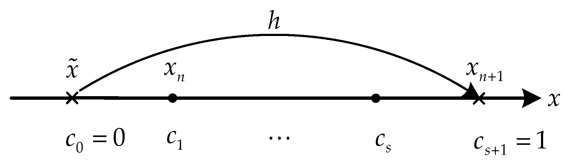
As is shown in Figure 2, let $x_{n-1}<\tilde{x}<x_n$, and divide the interval $x\in \left[\tilde{x}，x_{n+1}\right]$ into $s+1$ segments, in which $h=x_{n+1}-\tilde{x}$, $x(\tilde{x}+c_{0}h)\equiv \tilde{x}$, $x(\tilde{x}+c_{s}h)\equiv x_1$, $x(\tilde{x}+c_{s+1}h)\equiv x_{n+1}$.

Define

$$\upsilon =\{\begin{array}{l}s/2,\mathrm{for}\mathrm{even}s\hfill \\ (s+1)/2,\mathrm{for}\mathrm{odd}s\hfill \end{array}$$

(22)

then we can obtain the following formula according to Equation (12)

$$\tilde{\mathit{G}}\left[\begin{array}{c}{y}_n\\ ⋮\\ y_{n+\upsilon -1}\\ y_{n+\upsilon }\\ ⋮\\ y_{n+s}\end{array}\right]+{\mathit{G}}_{0}y(\tilde{x})=h\left[\begin{array}{c}{f}_n\\ ⋮\\ f_{n+\upsilon -1}\\ f_{n+\upsilon }\\ ⋮\\ f_{n+s}\end{array}\right]$$

(23)

in which $\tilde{\mathit{G}}\in R^{(s+1)\times (s+1)}$, ${\mathit{G}}_0\in R^{(s+1)\times 1}$; $y_{n+z}=y(\tilde{x}+c_{z+1}h),z\in (0,s)$.

In additional, define

$$\tilde{\mathit{A}}={\tilde{\mathit{G}}}^{-1}\equiv \left[{\tilde{a}}_{pq}\right],p,q\in (1,s+1)$$

(24)

Since it has been proved that [12,15]

$${\mathit{G}}_0=-\tilde{\mathit{G}}\mathit{e}$$

(25)

where, $\mathit{e}$ is the unit column vector, therefore, the Equation (23) can be rewritten as

$$\left[\begin{array}{c}{y}_n\\ ⋮\\ y_{n+\upsilon -1}\\ y_{n+\upsilon }\\ ⋮\\ y_{n+s}\end{array}\right]=y(\tilde{x})\mathit{e}+h\tilde{\mathit{A}}\left[\begin{array}{c}{f}_n\\ ⋮\\ f_{n+\upsilon -1}\\ f_{n+\upsilon }\\ ⋮\\ f_{n+s}\end{array}\right]$$

(26)

Subtracting the $\upsilon$-th equation from the $(\upsilon +1)$-th equation in the matrix Equation (26) yields the following equation

$$y_{n+\upsilon }-y_{n+\upsilon -1}=h{\displaystyle \sum _{z=0}^s{\beta }_z{f}_{n+z}}$$

(27)

where,

$${\beta }_z={\tilde{a}}_{\upsilon +1,z+1}-{\tilde{a}}_{\upsilon ,z+1},z\in (0,s)$$

(28)

It can be shown that the above numerical method (27) has the accuracy of $(s+1)$-order.

The numerical method (27) has a similar form to the traditional Adams methods, but we will later show that this method has the better numerical stability then traditional Adams methods. We call this numerical method the generalized Adams methods (GAMs).

When selecting the uniform grids, the coefficient values (${\beta }_z$) of GAMs are shown in the following

Table 4. Coefficients of generalized Adams methods (GAMs) using uniform grids (for even s).

s	v	β0	β1	β2	β3	β4	β5	β6
$2$	$1$	$\frac{5}{36}$	$\frac{2}{9}$	$-\frac{1}{36}$
$4$	$2$	$-\frac{19}{3600}$	$\frac{173}{1800}$	$\frac{19}{150}$	$-\frac{37}{1800}$	$\frac{11}{3600}$
$6$	$3$	$\frac{271}{423,360}$	$-\frac{23}{3528}$	$\frac{10,273}{141,120}$	$\frac{586}{6615}$	$-\frac{2257}{141,120}$	$\frac{67}{17,640}$	$-\frac{191}{423,360}$

and

Table 5. Coefficients of GAMs using uniform grids (for odd s).

s	v	β0	β1	β2	β3	β4	β5	β6	β7
$1$	$1$	$\frac{1}{4}$	$\frac{1}{4}$
$3$	$2$	$-\frac{1}{96}$	$\frac{13}{96}$	$\frac{13}{96}$	$-\frac{1}{96}$
$5$	$3$	$\frac{11}{8640}$	$-\frac{31}{2880}$	$\frac{401}{4320}$	$\frac{401}{4320}$	$-\frac{31}{2880}$	$\frac{11}{8640}$
$7$	$4$	$-\frac{191}{967,680}$	$\frac{1879}{967,680}$	$-\frac{353}{35,840}$	$\frac{68,323}{967,680}$	$\frac{68,323}{967,680}$	$-\frac{353}{35,840}$	$\frac{1879}{967,680}$	$-\frac{191}{967,680}$

respectively.

For the uniform grids, we can define that

$$\overline{h}=(x_{n+1}-\tilde{x})/(s+1)=h/(s+1)$$

(29)

therefore, the method (27) could be rewritten as

$$y_{n+\upsilon }-y_{n+\upsilon -1}=\overline{h}{\displaystyle \sum _{z=0}^s(\frac{{\beta }_z}{s+1})f_{n+z}}$$

(30)

According to Table 4 and Table 5, we can verify that the proposed method (30) is consistent with the GAMs proposed by Brugnano et al. [19]. In reference [21], it has been shown that, for even s, the methods (30) are both A-stable, and for odd s the methods (30) are also A-stable while the stability region is just the complete left half plane.

3.4. The Extended Trapezoidal Rules

3.4.1. Extended Trapezoidal Rules of the First Kind

As is shown in Figure 1, and let s be an odd number. Define

$$\upsilon =(s+1)/2$$

(31)

then we can obtain the following formula via DQM

$$\mathit{G}\left[\begin{array}{c}{y}_n\\ ⋮\\ y_{n+\upsilon -1}\\ y_{n+\upsilon }\\ ⋮\\ y_{n+s}\end{array}\right]=h\left[\begin{array}{c}{f}_n\\ ⋮\\ f_{n+\upsilon -1}\\ f_{n+\upsilon }\\ ⋮\\ f_{n+s}\end{array}\right],\mathit{G}\in R^{(s+1)\times (s+1)}$$

(32)

The same as Equation (12), Equation (32) is also the basic calculation scheme of DQM, however, the scheme of Equation (12) is more widely used in engineering application. In general, the matrix $\mathit{G}$ in Equation (32) is not a full rank matrix, so its inverse matrix does not exist.

If the distribution of grid points is centro-symmetrical in the normalized interval $[0,1]$, the matrix $\mathit{G}$ in Equation (32) will be a centro-antisymmetrical matrix. Since the inverse matrix of $\mathit{G}$ does not exist, it is natural to consider its generalized inverse matrix. As is well known, the generalized inverse matrix—namely, the pseudo-inverse matrix ${\mathit{G}}^{+}={\left({\mathit{G}}^{\mathrm{T}}\mathit{G}\right)}^{-1}{\mathit{G}}^{\mathrm{T}}$ of centro-antisymmetrical matrix with even order—will also be a centro-antisymmetrical matrix.

Define

$${\mathit{G}}^{+}=\mathit{A}\equiv \left[a_{pq}\right],p,q\in (1,s+1)$$

(33)

then the Equation (32) can be written as

$$\left[\begin{array}{c}{y}_n\\ ⋮\\ y_{n+\upsilon -1}\\ y_{n+\upsilon }\\ ⋮\\ y_{n+s}\end{array}\right]=h\mathit{A}\left[\begin{array}{c}{f}_n\\ ⋮\\ f_{n+\upsilon -1}\\ f_{n+\upsilon }\\ ⋮\\ f_{n+s}\end{array}\right]$$

(34)

Subtracting the $\upsilon$-th equation from the $(\upsilon +1)$-th equation in the matrix Equation (34), we can obtain the following equation

$$y_{n+\upsilon }-y_{n+\upsilon -1}=h{\displaystyle \sum _{z=0}^s{\rho }_z{f}_{n+z}}$$

(35)

It is obvious that the aforementioned Equation (35) is the GAMs with $(s+1)$-order, in which

$${\rho }_z=a_{\upsilon +1,z+1}-a_{\upsilon ,z+1},z\in (0,s)$$

(36)

Considering that $s=2\upsilon -1$ and $\mathit{A}$ defined in Equation (33) is a centro-antisymmetrical matrix with even dimension, it can be easily proved that ${\rho }_z$ in Equation (36) is centro-symmetrical. Therefore, Equation (35) can be further written as

$$y_{n+\upsilon +1}-y_{n+\upsilon }=h{\displaystyle \sum _{z=0}^{\upsilon -1}{\rho }_z(f_{n+z}+f_{n+s-z})}$$

(37)

When selecting the uniform grids, the values ${\rho }_z$ are listed in the following

Table 6. Coefficients of extended trapezoidal rules of the first kind (ETR₁) using uniform grids.

s	v	ρ0	ρ1	ρ2	ρ3	ρ4
$1$	$1$	$\frac{1}{2}$
$3$	$2$	$-\frac{1}{72}$	$\frac{13}{72}$
$5$	$3$	$\frac{11}{7200}$	$-\frac{31}{2400}$	$\frac{401}{3600}$
$7$	$4$	$-\frac{191}{846,720}$	$\frac{1,879}{846,720}$	$-\frac{353}{31,360}$	$\frac{68,323}{846,720}$
$9$	$5$	$\frac{2497}{65,318,400}$	$-\frac{28939}{65,318,400}$	$\frac{581}{233,280}$	$-\frac{40,111}{4,082,400}$	$\frac{2,067,169}{32,659,200}$

.

Obviously, when $s=1$, the aforementioned Equation (37) is just the classic implicit trapezoidal rule, so, we call this numerical method the extended trapezoidal rules of the first kind (ETR₁).

Although ETR₁ are simply the GAMs, the deduction method of these two methods is slightly different. Therefore, comparing Table 6 with Table 4, it can be clearly seen that the concrete results—i.e., the coefficients—are different.

It has been shown in reference [21] that the stability regions of ETR₁ methods are the same as that of the classic implicit trapezoidal integration rule, and they are all A-stable methods.

3.4.2. Extended Trapezoidal Rules of the Second Kind

Let s be an odd number, and the expression of $\upsilon$ is also the same with Equation (31). According to matrix Equation (12), it can be drawn that

$$\tilde{\mathit{G}}\left[\begin{array}{c}{y}_{n+1}\\ ⋮\\ y_{n+\upsilon -1}\\ y_{n+\upsilon }\\ ⋮\\ y_{n+s}\end{array}\right]+{\mathit{G}}_0{y}_n=h\left[\begin{array}{c}{f}_{n+1}\\ ⋮\\ f_{n+\upsilon -1}\\ f_{n+\upsilon }\\ ⋮\\ f_{n+s}\end{array}\right]$$

(38)

In the above matrix equation, add $(\upsilon -1)$-th equation to the $\upsilon$-th equation, we can get

$${\displaystyle \sum _{z=0}^s{\overline{\alpha }}_z{y}_{n+z}}=h(f_{n+\upsilon -1}+f_{n+\upsilon })$$

(39)

where,

$${\overline{\alpha }}_z=g_{\upsilon -1,z}+g_{\upsilon ,z},z\in (0,s)$$

(40)

Considering that $s=2\upsilon -1$, as well as the weighting coefficient g_pq is centro-antisymmetrical and ${\overline{\alpha }}_z$ is centro-antisymmetrical, the Equation (39) could lastly be written as

$${\displaystyle \sum _{z=0}^{\upsilon -1}{\omega }_z({\tilde{x}}_{n+z}-{\tilde{x}}_{n+s-z})}=\frac{h}{2}(f_{n+\upsilon -1}+f_{n+\upsilon })$$

(41)

where,

$${\omega }_z={\overline{\alpha }}_z/2=(g_{\upsilon -1,z}+g_{\upsilon ,z})/2,z\in (0,\upsilon -1)$$

(42)

When selecting the uniform grids, the coefficient values (${\omega }_z$) in Equation (41) are shown in the following

Table 7. Coefficients of extended trapezoidal rules of the second kind (ETR₂) using uniform grids.

s	v	ω0	ω1	ω2	ω3	ω4
$1$	$1$	$-1$
$3$	$2$	$-\frac{1}{4}$	$-\frac{9}{4}$
$5$	$3$	$\frac{1}{24}$	$-\frac{5}{8}$	$-\frac{10}{3}$
$7$	$4$	$-\frac{1}{120}$	$\frac{7}{60}$	$-\frac{21}{20}$	$-\frac{35}{8}$
$9$	$5$	$\frac{1}{560}$	$-\frac{3}{112}$	$\frac{3}{14}$	$-\frac{3}{2}$	$-\frac{27}{5}$

.

Obviously, when $s=1$, the aforementioned method is just the implicit trapezoidal method; thus, this numerical method can be named the extended trapezoidal rules of the second kind (ETR₂).

According to Table 7, it can be verified that the method (41) is consistent with ETR₂ methods that proposed by Brugnano et al. [19]. The stability regions of ETR₂ methods are the same with that of classic implicit trapezoidal integration rule, and they are all A-stable methods.

4. Fourier Stability Analysis for the Derived Compact Difference Schemes

Stability analysis is an important part of the numerical integration approach. In general, we use linear stability analysis by the use of a standard scalar test equation ($\dot{x}=\lambda x$) [21,22,23]. However, the linear stability analysis does not provide information about the performance of schemes at different length scales. Unlike this, the Fourier stability analysis provides an effective way to quantify the resolution characteristics such as dispersion or phase error of the differencing approximations. In this section, we analyze the dispersion and dissipation characteristics of the derived difference schemes using Fourier stability analysis [1,24].

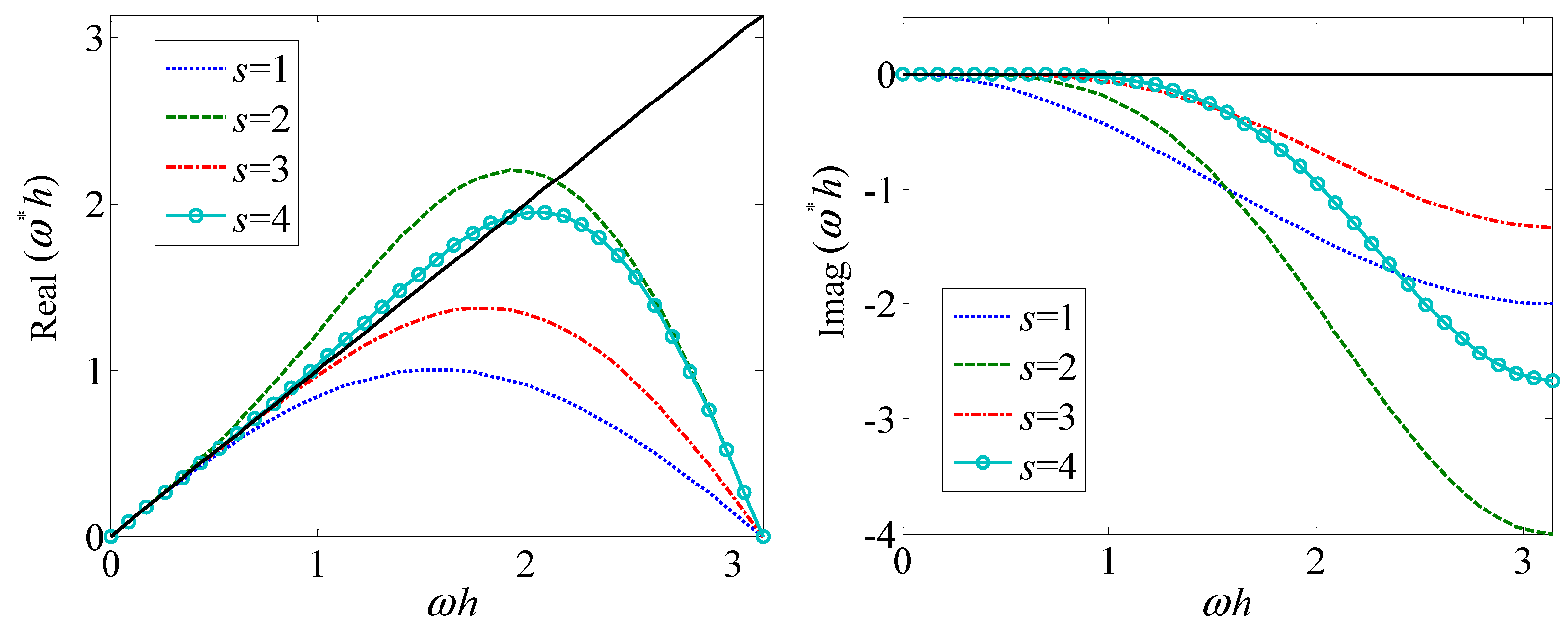
By the Fourier stability analysis, different numerical schemes have different estimates of the modified scaled wavenumber, and it is in general a complex quantity [25]. It can easily be shown that the real part of the modified scaled wavenumber tends to amplify/attenuate the corresponding Fourier mode while the imaginary part introduces a phase error. Thus the deviations of the real and imaginary parts of the modified scaled wavenumber from the exact scaled wavenumber can be respectively taken to be the indicators of numerical dissipation and dispersion. Furthermore, for numerical stability of any scheme, one must look at the imaginary part of the modified scaled wavenumber. The imaginary part of the modified scaled wavenumber represents numerical dissipation only when it is negative. Any scheme that produces a positive imaginary part of the modified scaled wavenumber is numerically unstable because a positive imaginary part is equivalent to adding anti-diffusion [25].

Figure 3 shows the modified scaled wavenumber of GBDF based on uniform grids.

Based on the above results, we can see that GBDF are all stable numerical methods, and this kind of method has a strong numerical dissipation and dispersion.

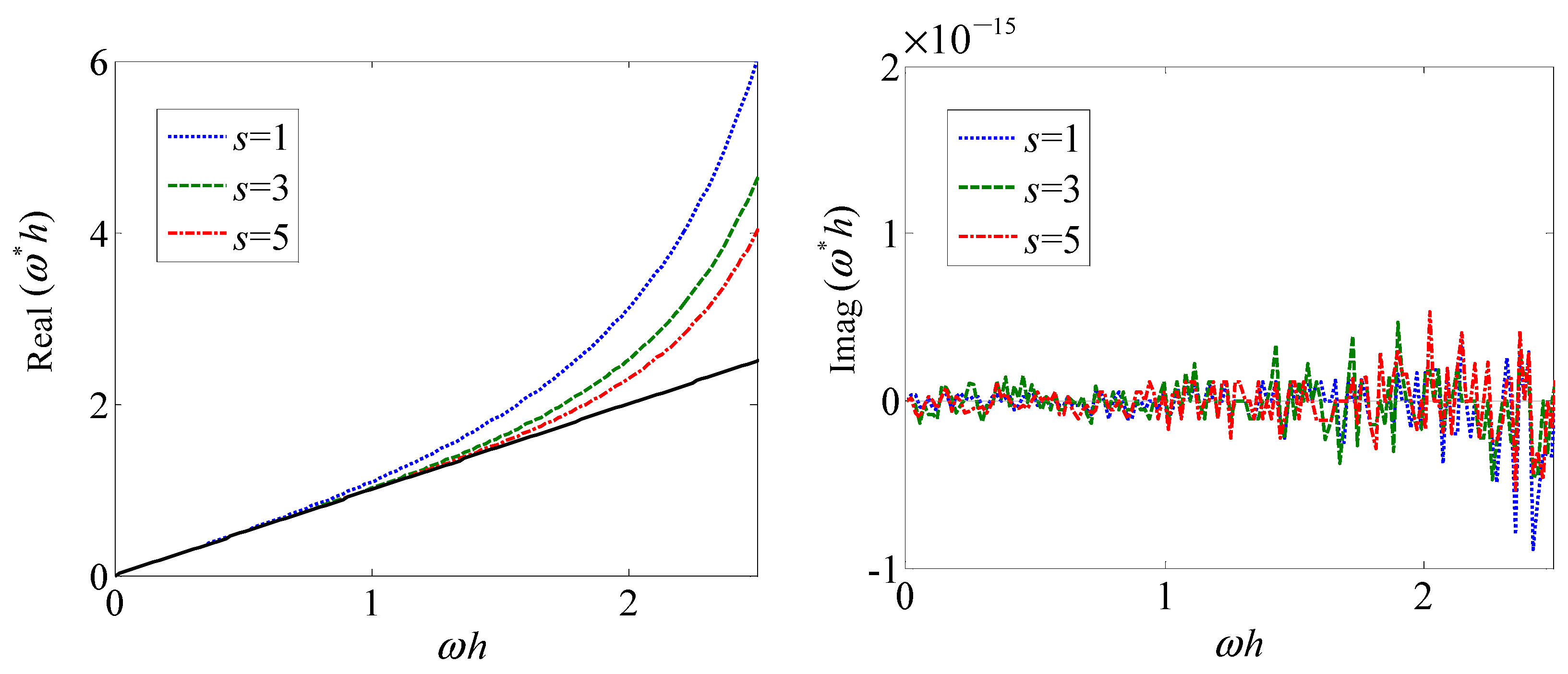
Figure 4 shows the modified scaled wavenumber of central compact difference schemes (CCDS) based on uniform grids.

Based on the above results, we can see that CCDS have a strong numerical dispersion but have almost no numerical dissipation.

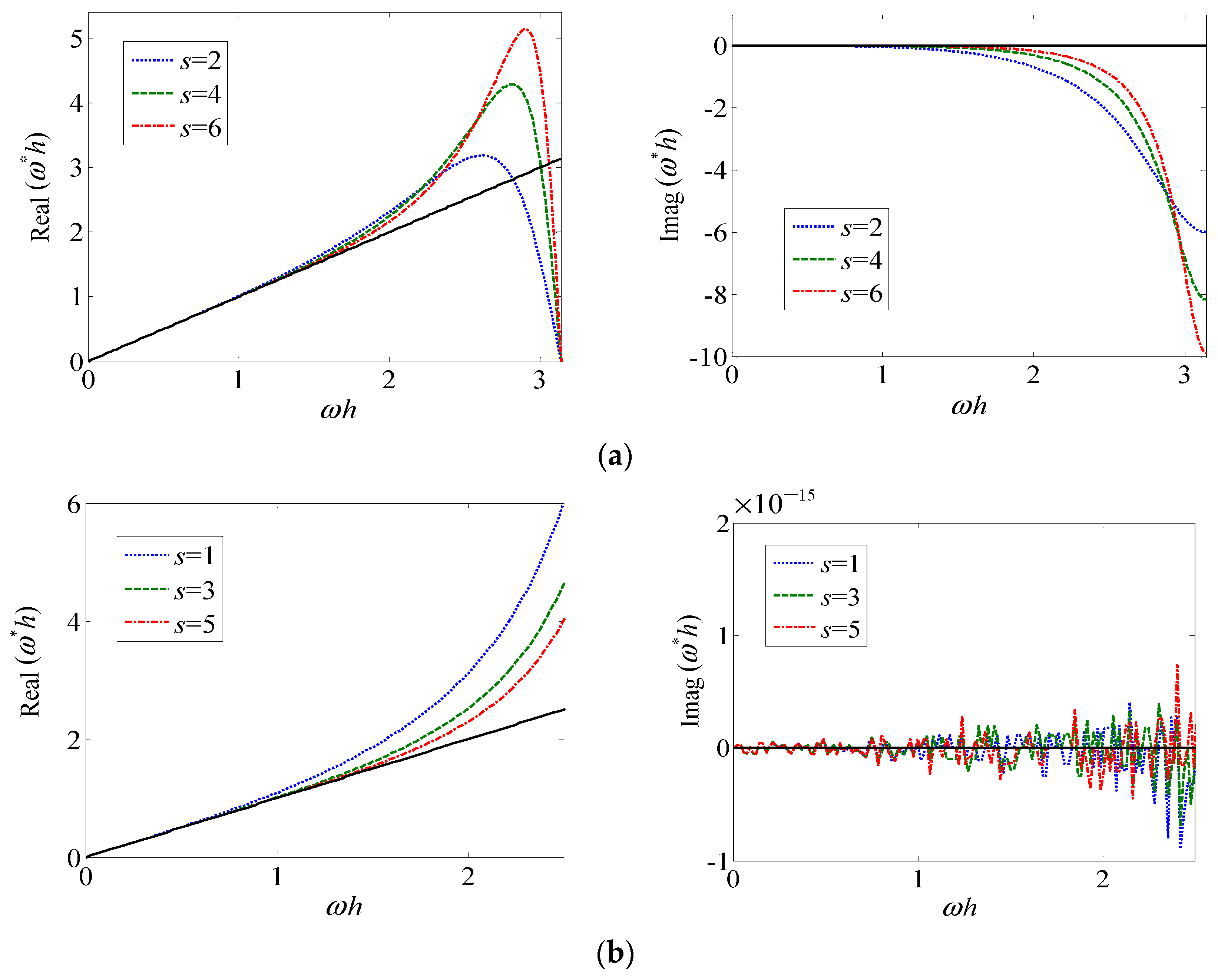
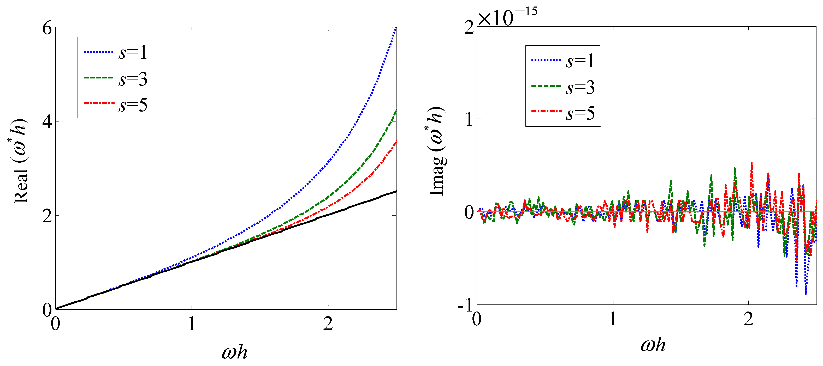
Figure 5a,b show the modified scaled wavenumber of GAMs based on uniform grids and respectively for even s and odd s.

Figure 6 shows the modified scaled wavenumber of ETR₁ based on uniform grids.

Based on the above results, we can see that the ETR₁ are roughly equivalent to the GAMs with odd s in terms of numerical dissipation and dispersion. In fact, as mentioned earlier, these two methods are essentially the same.

Figure 7 shows the modified scaled wavenumber of ETR₂ based on uniform grids.

Based on the above results, we can see that the ETR₂ are roughly equivalent to the ETR₁ and GAMs with odd s in terms of numerical dissipation and dispersion.

To sum up, from the perspective of numerical dissipation, the CCDS, GAMs with odd s, ETR1 and ETR2 methods perform better than the GAMs with even s and GBDF methods, but from the perspective of phase dispersion, the high-order GBDF methods behave slightly better than other methods. In the wavenumber range $\omega h\le 1$, the proposed methods both have a high numerical resolution.

From the practical application of the point of view, the above different schemes have different practical application scenarios. For example, the GBDF method may be a better choice for electromagnetic transient simulation of electric power systems, because the dissipation of this method could avoid or effectively dampen fictitious numerical oscillations caused by abrupt phenomena. However, for electromechanical transient simulation of electric power systems, the GBDF method is likely to yield the wrong result due to the strong numerical dissipation: a stable system of its own, the corresponding simulation results may be stable. Based on the above analysis results combined with our experience, the high-order scheme of GAMs with even s and CCDS could be a better choice for electromechanical transient simulation of electric power systems.

5. Conclusions

Using the classic differential quadrature formulae while adopting the uniform grid points, this paper has symmetrically constructed a variety of compact difference schemes. Although some of the constructed methods in this paper are consistent with the boundary value method proposed by Brugnano et al., they are completely different in the means of construction. In fact, based on the methods described in this paper, it is easy to construct the compact difference schemes based on second-order derivatives.

Using Fourier stability analysis method, the characteristics such as the dissipation, dispersion and resolution of the different schemes were studied and compared. Based on these results, it is found that the CCDS, GAMs with odd s, ETR₁ and ETR₂ have almost no numerical dissipation, and GAMs, ETR₁ and ETR₂ have a high resolution when the wave number is not very large. In summary, the derived compact difference schemes in this paper could be used instead of classic differential quadrature methods for engineering applications.