
Prediction of Critical Currents for a Diluted Square Lattice Using Artificial Neural Networks


Abstract
:
1. Introduction
2. Experimental Setup and Transport Measurements
2.1. Experimental Setup
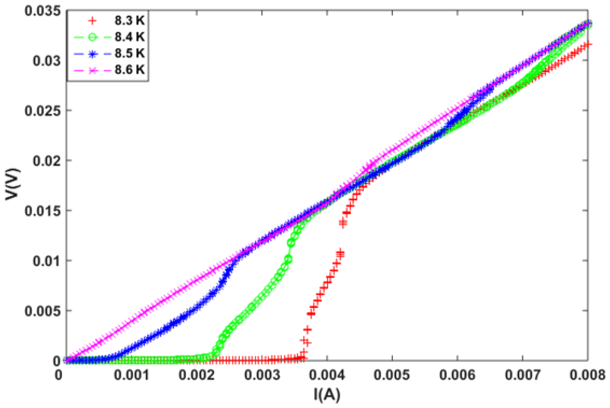
2.2. Measurements Using PPMS
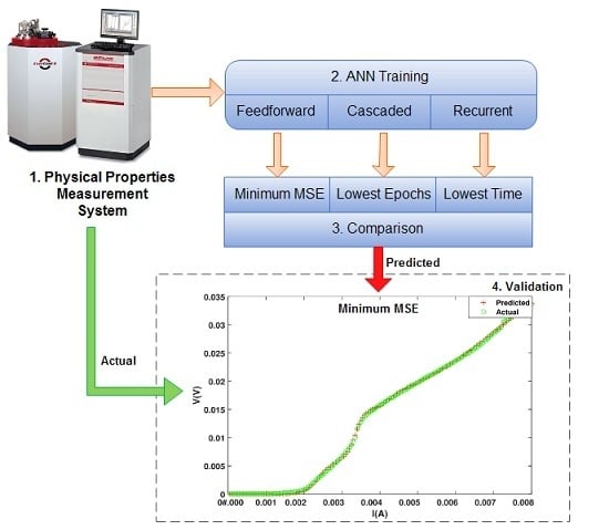
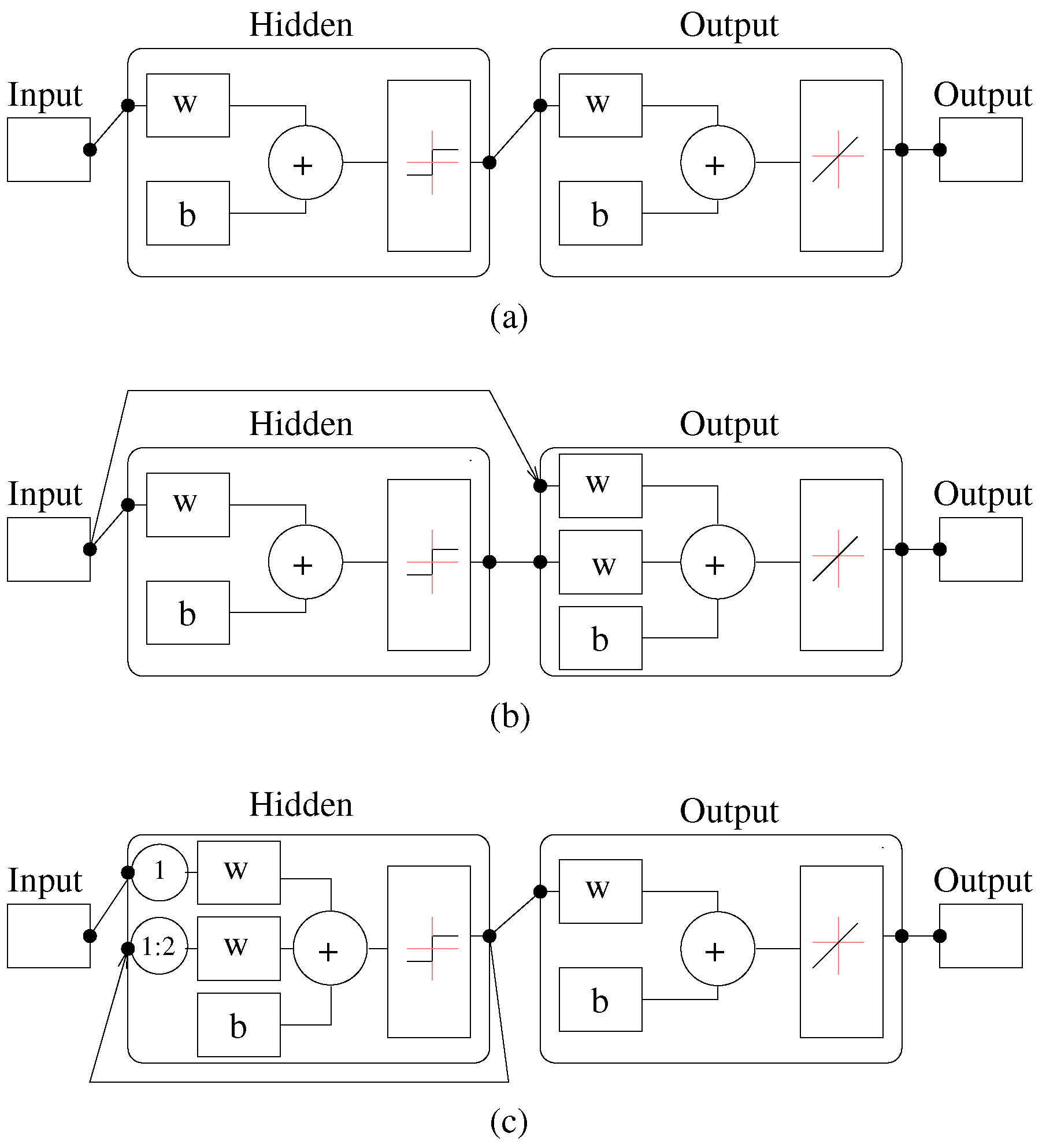
3. ANN Architectures and Training Algorithms
- represents the weights from neuron k in the second hidden layer to the output neurons.
- represents the weights from neuron j in the first hidden layer to neuron k in the second layer.
- represents the weights from neuron i in the input layer to the neuron j in the first hidden layer.
- represents the element in the input layer.
- , , and represent the bias values for the hidden and output layers.
- , and are the activation functions: H1, H2, and o stand for the first and second hidden and the output layers, respectively.The primary objective of this analysis is to minimize a cost function given by Equation (2):
3.1. Feedforward Networks
3.2. Cascade-Forward Networks
3.3. Layer-Recurrent Networks
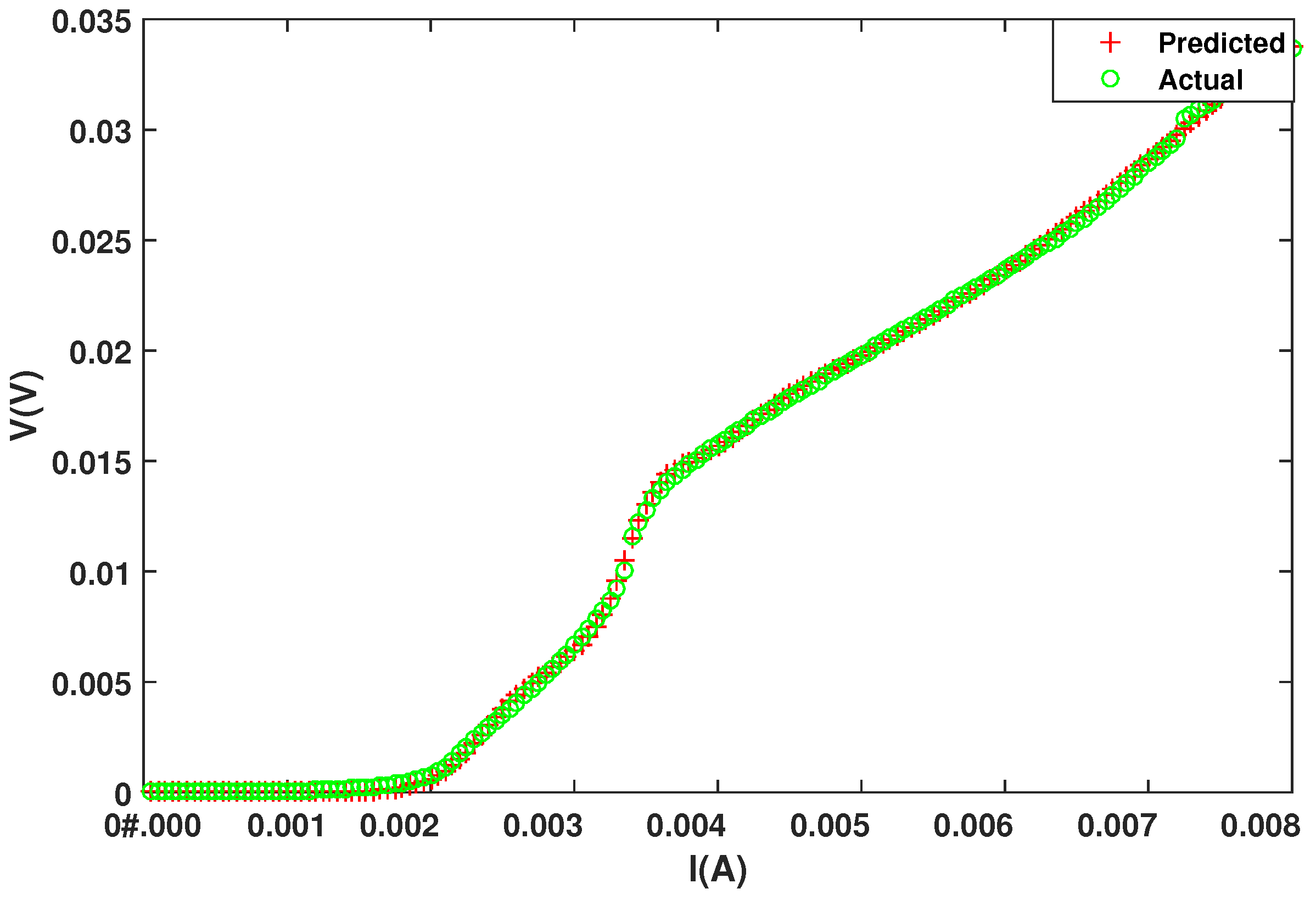
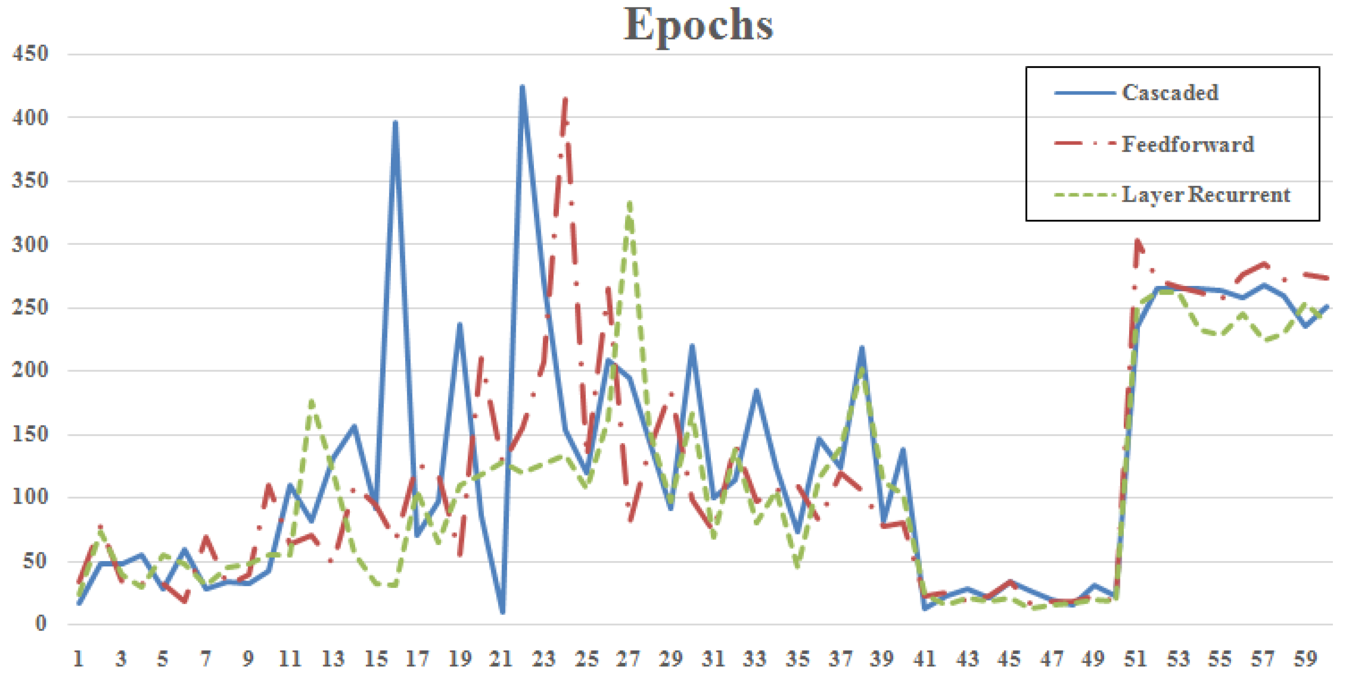
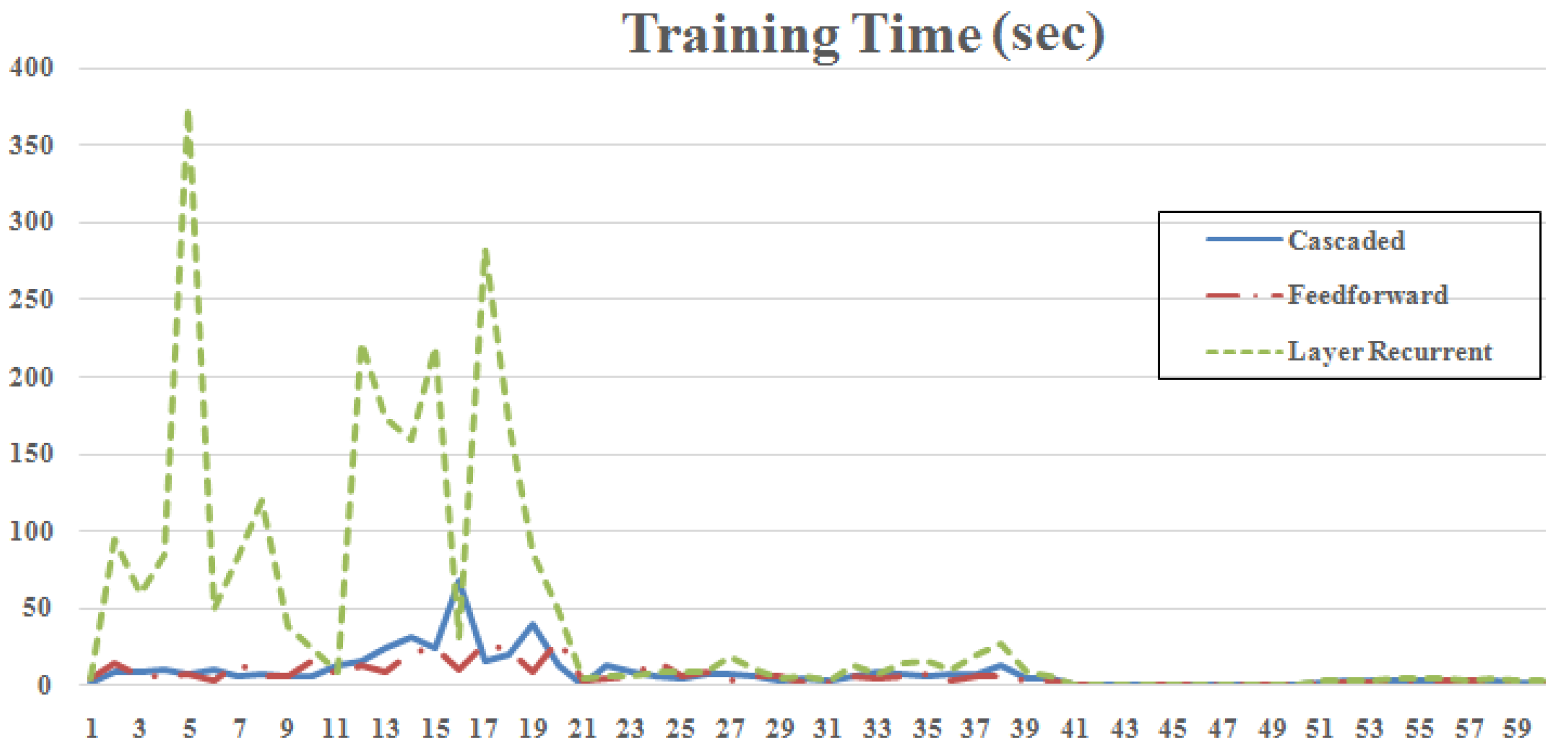
4. Simulation Results
5. Conclusions
Author Contributions
Conflicts of Interest
References
- Baert, M.; Metlushko, V.; Jonckheere, R.; Moshchalkov, V.; Bruynseraede, Y. Composite flux-line lattices stabilized in superconducting films by a regular array of artificial defects. Phys. Rev. Lett. 1995, 74, 3269. [Google Scholar] [CrossRef] [PubMed]
- Martin, J.I.; Vélez, M.; Hoffmann, A.; Schuller, I.K.; Vicent, J. Artificially induced reconfiguration of the vortex lattice by arrays of magnetic dots. Phys. Rev. Lett. 1999, 83, 1022. [Google Scholar] [CrossRef]
- Latimer, M.; Berdiyorov, G.; Xiao, Z.; Kwok, W.; Peeters, F. Vortex interaction enhanced saturation number and caging effect in a superconducting film with a honeycomb array of nanoscale holes. Phys. Rev. B 2012, 85, 012505. [Google Scholar] [CrossRef]
- Villegas, J.; Savel’ev, S.; Nori, F.; Gonzalez, E.; Anguita, J.; Garcia, R.; Vicent, J. A superconducting reversible rectifier that controls the motion of magnetic flux quanta. Science 2003, 302, 1188–1191. [Google Scholar] [CrossRef] [PubMed]
- Kamran, M.; Naqvi, S.R.; Kiani, F.; Basit, A.; Wazir, Z.; He, S.K.; Zhao, S.P.; Qiu, X.G. Absence of Reconfiguration for Extreme Periods of Rectangular Array of Holes. J. Supercond. Novel Magn. 2015, 28, 3311–3315. [Google Scholar] [CrossRef]
- Martin, J.I.; Vélez, M.; Nogues, J.; Schuller, I.K. Flux pinning in a superconductor by an array of submicrometer magnetic dots. Phys. Rev. Lett. 1997, 79, 1929. [Google Scholar] [CrossRef] [Green Version]
- Jaccard, Y.; Martin, J.; Cyrille, M.C.; Vélez, M.; Vicent, J.; Schuller, I.K. Magnetic pinning of the vortex lattice by arrays of submicrometric dots. Phys. Rev. B 1998, 58, 8232. [Google Scholar] [CrossRef]
- Cuppens, J.; Ataklti, G.; Gillijns, W.; Van de Vondel, J.; Moshchalkov, V.; Silhanek, A. Vortex dynamics in a superconducting film with a kagomé and a honeycomb pinning landscape. J. Supercond. Novel Magn. 2011, 24, 7–11. [Google Scholar] [CrossRef]
- De Lara, D.P.; Alija, A.; Gonzalez, E.; Velez, M.; Martin, J.; Vicent, J.L. Vortex ratchet reversal at fractional matching fields in kagomélike array with symmetric pinning centers. Phys. Rev. B 2010, 82, 174503. [Google Scholar] [CrossRef]
- He, S.; Zhang, W.; Liu, H.; Xue, G.; Li, B.; Xiao, H.; Wen, Z.; Han, X.; Zhao, S.; Gu, C.; et al. Wire network behavior in superconducting Nb films with diluted triangular arrays of holes. J. Phys. Condens. Matter 2012, 24, 155702. [Google Scholar] [CrossRef] [PubMed]
- Kamran, M.; Haider, S.; Akram, T.; Naqvi, S.; He, S. Prediction of IV curves for a superconducting thin film using artificial neural networks. Superlattices Microstruct. 2016, 95, 88–94. [Google Scholar] [CrossRef]
- Guojin, C.; Miaofen, Z.; Honghao, Y.; Yan, L. Application of Neural Networks in Image Definition Recognition. In Proceedings of the IEEE International Conference on Signal Processing and Communications, Dubai, UAE, 24–27 November 2007; pp. 1207–1210.
- Güçlü, U.; van Gerven, M.A.J. Deep Neural Networks Reveal a Gradient in the Complexity of Neural Representations across the Ventral Stream. J. Neurosci. 2015, 35, 10005–10014. [Google Scholar] [CrossRef] [PubMed] [Green Version]
- Cybenko, G. Approximation by superpositions of a sigmoidal function. Math. Control Signals Syst. 1989, 2, 303–314. [Google Scholar] [CrossRef]
- Hornik, K. Approximation capabilities of multilayer feedforward networks. Neural Netw. 1991, 4, 251–257. [Google Scholar] [CrossRef]
- Hornik, K. Some new results on neural network approximation. Neural Netw. 1993, 6, 1069–1072. [Google Scholar] [CrossRef]
- Hornik, K.; Stinchcombe, M.; White, H. Multilayer feedforward networks are universal approximators. Neural Netw. 1989, 2, 359–366. [Google Scholar] [CrossRef]
- Bielecki, A.; Ombach, J. Dynamical properties of a perceptron learning process: Structural stability under numerics and shadowing. J. Nonlinear Sci. 2011, 21, 579–593. [Google Scholar] [CrossRef]
- Meireles, M.; Almeida, P.; Simoes, M. A comprehensive review for industrial applicability of artificial neural networks. IEEE Trans. Ind. Electr. 2003, 50, 585–601. [Google Scholar] [CrossRef]
- Üreyen, M.E.; Gürkan, P. Comparison of artificial neural network and linear regression models for prediction of ring spun yarn properties. I. Prediction of yarn tensile properties. Fibers Polym. 2008, 9, 87–91. [Google Scholar] [CrossRef]
- Ghanbari, A.; Naghavi, A.; Ghaderi, S.; Sabaghian, M. Artificial Neural Networks and regression approaches comparison for forecasting Iran’s annual electricity load. In Proceedings of the International Conference on Power Engineering, Energy and Electrical Drives, Lisbon, Portugal, 18–20 March 2009; pp. 675–679.
- Elminir, H.K.; Azzam, Y.A.; Younes, F.I. Prediction of hourly and daily diffuse fraction using neural network, as compared to linear regression models. Energy 2007, 32, 1513–1523. [Google Scholar] [CrossRef]
- Quan, G.Z.; Pan, J.; Wang, X. Prediction of the Hot Compressive Deformation Behavior for Superalloy Nimonic 80A by BP-ANN Model. Appl. Sci. 2016, 6, 66. [Google Scholar] [CrossRef]
- Zhao, M.; Li, Z.; He, W. Classifying Four Carbon Fiber Fabrics via Machine Learning: A Comparative Study Using ANNs and SVM. Appl. Sci. 2016, 6, 209. [Google Scholar] [CrossRef]
- Odagawa, A.; Sakai, M.; Adachi, H.; Setsune, K.; Hirao, T.; Yoshida, K. Observation of intrinsic Josephson junction properties on (Bi, Pb) SrCaCuO thin films. Jpn. J. Appl. Phys. 1997, 36, L21. [Google Scholar] [CrossRef]
- Setti, S.G.; Rao, R. Artificial neural network approach for prediction of stress–strain curve of near β titanium alloy. Rare Met. 2014, 33, 249–257. [Google Scholar] [CrossRef]
- Marquardt, D.W. An algorithm for least-squares estimation of nonlinear parameters. J. Soc. Ind. Appl. Math. 1963, 11, 431–441. [Google Scholar] [CrossRef]
- MacKay, D.J. A practical Bayesian framework for backpropagation networks. Neural Comput. 1992, 4, 448–472. [Google Scholar] [CrossRef]
- Beale, E. A derivation of conjugate gradients. In Numerical Methods for Nonlinear Optimization; Academic Press Inc.: Cambridge, MA, USA, 1972; pp. 39–43. [Google Scholar]
- Gill, P.E.; Murray, W.; Wright, M.H. Practical Optimization; Emerald Group Publishing Limited: Bingley, UK, 1981. [Google Scholar]
- Hestenes, M.R. Conjugate Direction Methods in Optimization; Springer Science & Business Media: New York, NY, USA, 2012; Volume 12. [Google Scholar]
- Johansson, E.M.; Dowla, F.U.; Goodman, D.M. Backpropagation learning for multilayer feed-forward neural networks using the conjugate gradient method. Int. J. Neural Syst. 1991, 2, 291–301. [Google Scholar] [CrossRef]
- Powell, M.J.D. Restart procedures for the conjugate gradient method. Math. Program. 1977, 12, 241–254. [Google Scholar] [CrossRef]
- Battiti, R.; Masulli, F. BFGS optimization for faster and automated supervised learning. In International Neural Network Conference; Springer: Berlin/Heidelberg, Germany, 1990; pp. 757–760. [Google Scholar]
- Beale, M.H.; Hagan, M.T.; Demuth, H.B. Neural network toolbox 7. In Matlab’s User Guide; Mathworks: Natick, MA, USA, 2010. [Google Scholar]


| I | V | I | V | I | V | I | V |
|---|---|---|---|---|---|---|---|
| 2.0 | 5.0 | 2.0 | 1.5 | 2.0 | −6.7 | 2.0 | −6.3 |
| 5.0 | 5.1 | 5.0 | 4.0 | 5.0 | 3.5 | 5.0 | 3.8 |
| 1.0 | 5.2 | 1.0 | 4.0 | 1.0 | 3.5 | 1.0 | 3.7 |
| 1.5 | 5.1 | 1.5 | 4.1 | 1.5 | 3.4 | 1.5 | 3.4 |
| 2.0 | 5.1 | 2.0 | 3.9 | 2.0 | 3.6 | 2.0 | 3.5 |
| 2.5 | 5.1 | 2.5 | 4.1 | 2.5 | 3.5 | 2.5 | 3.8 |
| 0H (Oe) | 100H (Oe) | 200H (Oe) | 300H (Oe) | ||||
| (a) | |||||||
| 5.0 | 5.1 | 5.0 | 4.0 | 5.0 | 3.8 | 5.0 | 4.4 |
| 1.0 | 5.0 | 1.0 | 3.9 | 1.0 | 3.6 | 1.0 | 4.4 |
| 1.5 | 5.0 | 1.5 | 3.9 | 1.5 | 3.7 | 1.5 | 4.3 |
| 2.0 | 5.0 | 2.0 | 3.9 | 2.0 | 3.7 | 2.0 | 4.2 |
| 2.5 | 5.1 | 2.5 | 4.1 | 2.5 | 3.6 | 2.5 | 4.1 |
| 0H (Oe) | 100H (Oe) | 200H (Oe) | 300H (Oe) | ||||
| (b) | |||||||
| Model | No. of | Train. | Model | No. of | Train. | Model | No. of | Train. |
|---|---|---|---|---|---|---|---|---|
| No. | Neurons | Algo. | No. | Neurons | Algo. | No. | Neurons | Algo. |
| 1. | [5 2] | LM | 21. | [5 2] | CGF | 41. | [5 2] | NR |
| 2. | [10 8] | LM | 22. | [10 8] | CGF | 42. | [10 8] | NR |
| 3. | [12 6] | LM | 23. | [12 6] | CGF | 43. | [12 6] | NR |
| 4. | [15 6] | LM | 24. | [15 6] | CGF | 44. | [15 6] | NR |
| 5. | [18 10] | LM | 25. | [18 10] | CGF | 45. | [18 10] | NR |
| 6. | [11 5] | LM | 26. | [11 5] | CGF | 46. | [11 5] | NR |
| 7. | [12 10] | LM | 27. | [12 10] | CGF | 47. | [12 10] | NR |
| 8. | [14 7] | LM | 28. | [14 7] | CGF | 48. | [14 7] | NR |
| 9. | [10 5] | LM | 29. | [10 5] | CGF | 49. | [10 5] | NR |
| 10. | [8 4] | LM | 30. | [8 4] | CGF | 50. | [8 4] | NR |
| 11. | [5 2] | BR | 31. | [5 2] | BFGS | 51. | [5 2] | GDX |
| 12. | [10 8] | BR | 32. | [10 8] | BFGS | 52. | [10 8] | GDX |
| 13. | [12 6] | BR | 33. | [12 6] | BFGS | 53. | [12 6] | GDX |
| 14. | [15 6] | BR | 34. | [15 6] | BFGS | 54. | [15 6] | GDX |
| 15. | [18 10] | BR | 35. | [18 10] | BFGS | 55. | [18 10] | GDX |
| 16. | [11 5] | BR | 36. | [11 5] | BFGS | 57. | [12 10] | GDX |
| 18. | [14 7] | BR | 38. | [14 7] | BFGS | 58. | [14 7] | GDX |
| 19. | [10 5] | BR | 39. | [10 5] | BFGS | 59. | [10 5] | GDX |
| 20. | [8 4] | BR | 40. | [8 4] | BFGS | 60. | [8 4] | GDX |
| Parameter | Network | No. of Neurons | Algo. | MSE | Epochs | Training Time (s) |
|---|---|---|---|---|---|---|
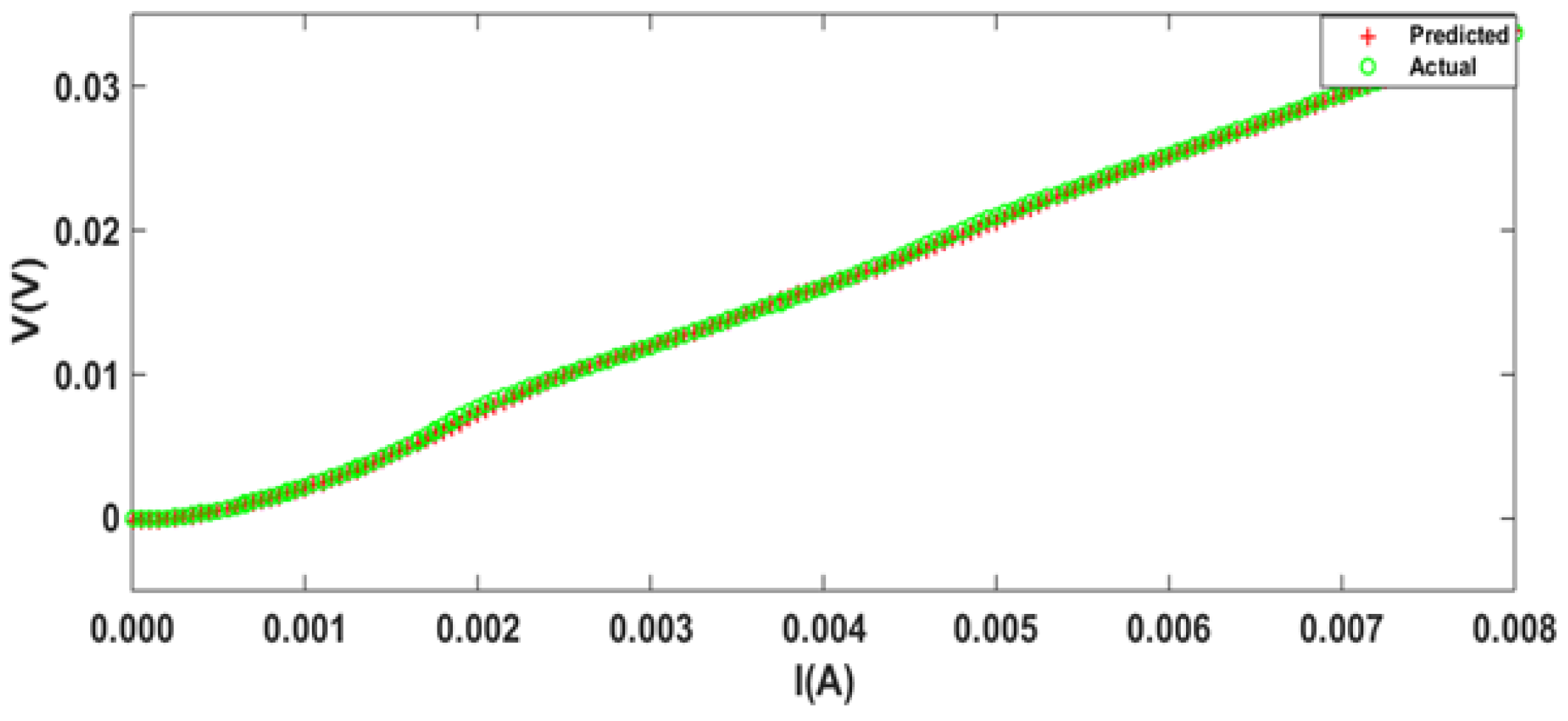
| Minimum MSE | Feedforward | [12 10] | BR | 4.55 | 126 | 26.037 |
| Minimum Epochs | Cascaded | [5 2] | CGF | 2.80 | 9 | 0.297 |
| Minimum Time | Feedforward | [8 4] | NR | 2.27 | 17 | 0.109 |
© 2017 by the authors. Licensee MDPI, Basel, Switzerland. This article is an open access article distributed under the terms and conditions of the Creative Commons Attribution (CC BY) license ( http://creativecommons.org/licenses/by/4.0/).
Share and Cite
Haider, S.A.; Naqvi, S.R.; Akram, T.; Kamran, M. Prediction of Critical Currents for a Diluted Square Lattice Using Artificial Neural Networks. Appl. Sci. 2017, 7, 238. https://doi.org/10.3390/app7030238
Haider SA, Naqvi SR, Akram T, Kamran M. Prediction of Critical Currents for a Diluted Square Lattice Using Artificial Neural Networks. Applied Sciences. 2017; 7(3):238. https://doi.org/10.3390/app7030238
Chicago/Turabian StyleHaider, Sajjad Ali, Syed Rameez Naqvi, Tallha Akram, and Muhammad Kamran. 2017. "Prediction of Critical Currents for a Diluted Square Lattice Using Artificial Neural Networks" Applied Sciences 7, no. 3: 238. https://doi.org/10.3390/app7030238