Robust Backstepping Control of Wing Rock Using Disturbance Observer

Abstract

Wing rock is a highly nonlinear phenomenon when the aircraft suffers undesired roll-dominated oscillatory at high angle of attack (AOA). Considering the strong nonlinear and unsteady aerodynamic characteristics, an uncertain multi-input and multi-output (MIMO) nonlinear wing rock model is studied, and system uncertainties, unsteady aerodynamic disturbances and external disturbances are considered in the design of wing rock control law. To handle the problem of multiple disturbances, a robust control scheme is proposed based on the extended state observer (ESO) and the radial basis function neural network (RBFNN) technique. Considering that the effectiveness of actuators are greatly decreased at high AOA, the input saturation problem is also handled by constructing a corresponding auxiliary system. Based on the improved ESO and the auxiliary system, a robust backstepping control law is proposed for the wing rock control. In addition, the dynamic surface control (DSC) technique is introduced to avoid the tedious computations of time derivatives for the virtual control laws in the backstepping method. The stability of the closed-loop system is guaranteed via rigorously Lyapunov analysis. Finally, simulation results are presented to illustrate the effectiveness of the ESO and the proposed wing rock control approach.

1. Introduction

Wing rock motion is an undesired roll-dominated oscillatory coupled with yaw oscillation for the aircraft flying at subsonic speed and high angle of attack (AOA). When an aircraft suffers the wing rock motion, the large amplitude and high frequency oscillatory of the rolling and yawing angle will severely limit the maneuverability, tracking accuracy, and operational safety of the aircraft. Hence, the wing rock phenomenon should be paid more attention, and the corresponding wing rock controller should be further studied.

In past decades, many researches have been done to analyze the mechanism of the wing rock. Mathematically, three possible nonlinear factors were considered as the inducements of the wing rock phenomenon, which are the variation of damping in roll with angle of sideslip, cubic variation of lateral derivatives with roll rate and sideslip, and the aerodynamic hysteresis in steady-state rolling moment [1,2]. Meanwhile, different wing-rock models have been developed [3,4,5,6]. Based on these simplified models, many control schemes were developed to suppress the influence of wing rock. Adaptive feedback linearization technique was employed for the wing rock in [7,8]. An $L_1$ adaptive controller was designed for the wing-body rock motion [9]. Fuzzy adaptive approaches have been employed in the wing rock during the last decade [10,11,12]. The neural network technique and backstepping approach have been also extensively studied [13,14,15]. In [16,17,18], simplified single degree-of-freedom wing-rock models were studied, and the disturbance observer or traditional extended state observer (ESO) was adopted in the design of robust wing rock control law. However, the yaw oscillation was often ignored in the design of wing rock controller for the convenience of research. Considering the serious coupling effect between the roll and yaw motion, multi-degree-of-freedom wing rock models should be further studied.

In this paper, an uncertain multi-input and multi-output (MIMO) nonlinear wing rock model is studied, and the coupling effect between the roll oscillation and yaw oscillation will be fully considered in the design of the wing rock controller. Meanwhile, to enhance the system robustness, the ESO and radial basis function neural network (RBFNN) techniques are combined to tackle the external disturbances and system uncertainties, respectively. Up to now, more and more researchers have paid attention to the study of the ESO or RBFNN based control techniques [19,20,21]. In [22], an adaptive neural network based control law was developed for an uncertain MIMO system with unknown control coefficient matrices and input nonlinearities. In [23], the observer and adaptive neural network (NN) techniques were combined to tackle the uncertainties. To tackle the state constraint problem, the adaptive neural network technique was employed for an uncertain robot system [24]. And the ESO technique was firstly proposed in the active disturbance rejection control (ADRC) [25]. It has been successfully used in many challenging engineering problems [26,27]. The main advantage of the traditional ESO is that it can handle various disturbances with little model information, and it takes both structured and unstructured uncertainties as generalized disturbances. Hence, considering the satisfactory uncertainty estimation performance, the ESO and RBFNN are fully combined in the design of the robust wing-rock control law. Meanwhile, except for uncertainties, the input saturation problem will also cause adverse effects on the performance of the wing rock control.

Input saturation is a challenging problem in the wing rock control. With the increase of AOA, the aircraft will lose the control efficiency gradually, which severely degrades the closed-loop system performance. During the past decades, there exist extensive researches on the control of mechanical systems with input saturation [28,29,30]. In [31], an adaptive neural tracking control was considered for a class of stochastic nonlinear systems with input saturation, and a smooth nonaffine function of the control input signal was designed to approximate the input saturation function. In [32], a modified fault tolerant control law was designed to handle the input saturation problem. Constrained adaptive backstepping control was proposed based on the command filters in [33]. Inspired by [34], the auxiliary system is designed to weaken the influence of the input saturation based on the backstepping technique in this paper.

The backstepping design method has been widely employed in the control of nonlinear systems. In recent years, many robust control methods have been introduced to combine with backstepping technique for the uncertain MIMO nonlinear systems [35,36,37,38,39]. However, the ESO-based robust backstepping technique should be further developed for the wing-rock motion due to the relatively easy realization. Inspired by the above discussions, a robust attitude tracking control law is proposed for the wing-rock motion in the presence of unsteady aerodynamic disturbances, external disturbances, system uncertainties and input saturation.

In this paper, considering the characters of different disturbances, efficient processing methods are adopted. The system uncertainty is estimated online by adaptive RBFNN. By taking full advantage of the output of the RBFNN and the known model information of the unsteady aerodynamic disturbance, the ESO is employed to estimate the compounded disturbance, which consists of the unsteady aerodynamic disturbance, external disturbance, and the unknown neural network approximation error. By making full use of the known information of the system, the disturbance estimation performance will be greatly improved. In addition, it is meaningful in the wing rock control at high AOA.

The paper is organized as follows. Problem formulation and preliminaries are described in Section 2. Section 3 presents the detailed design process of the disturbance observers. In Section 4, the robust backstepping wing rock control law is developed considering the input saturation. In Section 5, simulation results are given to demonstrate the effectiveness of the proposed robust tracking control scheme, followed by concluding remarks in Section 6.

2. Problem Formulation and Preliminaries

2.1. Problem Statement

According to the typical characteristics of wing rock motion, the following nonlinear MIMO lateral attitude motion model is considered [40]:

$$\begin{array}{ccc}\hfill {\dot{x}}_1& =& f_1(x_1)+g_1(x_1)x_2+\Delta f\left(x_1\right)+d_1\left(t\right)\hfill \\ \hfill {\dot{x}}_2& =& f_2(x_1,x_2)+g_2(x_1,x_2)u(v)+\Delta f_2(x_1,x_2)+G_2^{\prime }{h}_2+d_2\left(t\right)\hfill \\ \hfill y& =& x_1\hfill \end{array}$$

(1)

where $x_1={\left[\beta ,\mu \right]}^T\in R^2$ is an attitude angle vector which includes sideslip angle and flight-path roll angle, respectively; $x_2={\left[p,r\right]}^T\in R^2$ is the body-axis angular rate vector; y is the output; $f_1(x_1)\in R^2$, $f_2(x_1,x_2)\in R^2$ are known nonlinear function vectors; $g_1(x_1)\in R^{2\times 2}$, $g_2(x_1,x_2)\in R^{2\times 2}$, $G_2^{\prime }\in R^{2\times 2}$ are known invertible function matrices; $\Delta f_1(x_1)$ and $\Delta f_2(x_1,x_2)$ are the system uncertainties which include the modeling errors and the perturbation of aerodynamic coefficients; $d_1(t)$, $d_2(t)$ are the unknown external disturbance vectors; $v={\left[v_1,v_2\right]}^T$ is the designed control input; $u\left(v\right)={\left[u_1\left(v_1\right),u_2\left(v_2\right)\right]}^T={\left[{\delta }_a,{\delta }_y\right]}^T$ denotes the practical control input; ${\delta }_a$ is the aileron deflection angle and ${\delta }_y$ is the lateral thrust vectoring angle; $h_2={\left[h_l,h_n\right]}^T\in R^2$ is the unsteady moment aerodynamic coefficient vector, and $h_l,h_n$ are unsteady rolling moment aerodynamic coefficient and unsteady yawing moment aerodynamic coefficient, respectively.

On the basis of work in [41], the unsteady aerodynamic coefficient can be modeled by first-order linear differential equation which is given by

$${\dot{h}}_2=-B_2\left(\beta \right)h_2-A_2\left(\beta \right){\dot{x}}_1$$

(2)

where $B_2\left(\beta \right)=diag\left\{b_{21}\left(\beta \right),b_{22}\left(\beta \right)\right\}$, $A_2\left(\beta \right)=\left[\begin{array}{cc}{a}_{21}\left(\beta \right)& 0\\ a_{22}\left(\beta \right)& 0\end{array}\right]$, and $b_{21}\left(\beta \right)>0,b_{22}\left(\beta \right)>0,a_{21}\left(\beta \right),a_{22}\left(\beta \right)$ are known bounded function variables of β.

At high AOA, the lateral attitude motion of (1) becomes unstable. When system (1) suffers no disturbances, simulation results for an angle of attack of ${55}^{\circ }$ with initial conditions of ${\left[\beta \left(0\right),\mu \left(0\right)\right]}^T={\left[5^{\circ },0^{\circ }\right]}^T$, ${\left[p\left(0\right),r\left(0\right)\right]}^T={\left[0^{\circ }/s,0^{\circ }/s\right]}^T$ are given in Figure 1 and Figure 2. From Figure 1 and Figure 2, it can be observed that the roll angle exhibits large amplitude oscillatory motion, and the sideslip angle motion also exhibits considerable oscillation. Meanwhile, the maximum amplitude of the sideslip motion is closed to 20°, which is very dangerous for aircrafts at high AOA.

When system (1) suffers the disturbances, simulation results for an angle of attack of ${55}^{\circ }$ with initial conditions of ${\left[\beta \left(0\right),\mu \left(0\right)\right]}^T={\left[5^{\circ },0^{\circ }\right]}^T$, ${\left[p\left(0\right),r\left(0\right)\right]}^T={\left[0^{\circ }/s,0^{\circ }/s\right]}^T$ are given in Figure 3 and Figure 4. And the equations of the system uncertainty, unsteady aerodynamic disturbance and external disturbance will be given in details in the simulation section. In Figure 3 and Figure 4, the states of the aircraft diverge quickly, then stable wing rock appears after 50 s. Comparing Figure 3 and Figure 4 with Figure 1 and Figure 2, it can be concluded that the disturbances will further aggravate the oscillation. Thus, it is very important to design a robust controller to suppress the wing-rock motion, and render the roll angle and sideslip angle converge to zero quickly.

Considering that the wing rock motion is characterized by uncommanded roll-dominated oscillatory coupled with yaw oscillation, the aileron deflection angle ${\delta }_a$ and the lateral thrust vectoring angle ${\delta }_y$ are chosen as the practical control input. However, with the increase of AOA, the aileron control efficiency is reduced drastically [40]. Hence, the input saturation must be taken into consideration in the wing rock control. And the input saturation model can be written as

$$u_i\left(v_i\right)=sat\left(v_i\right)=\left\{\begin{array}{cc}sign\left(v_i\right)u_{M_i},\hfill & \left|v_i\right|\ge u_{M_i}\hfill \\ v_i,\hfill & \left|v_i\right|<u_{M_i}\hfill \end{array}\right.$$

(3)

where $u_{M_i}$ is the bounds of $u_i(t)$, i = 1, 2.

2.2. Neural Networks

The RBFNN has been widely employed to tackle unknown nonlinear functions due to its satisfactory approximation ability. Considering an unknown function $f\left(x\right):R^m\to R$, the RBFNN approximation output over a compact set ${\mathrm{\Omega }}_m\subseteq R^m$ can be written as [22]

$$f(x)=W^{{*}^T}S(x)+{\iota }^{*}$$

(4)

where $W^{*}\in R^p$ is the optimal weight value and ${\iota }^{*}$ is the smallest approximation error; $S(x)={[s_1(x),s_2(x),\cdots ,s_p(x)]}^T\in R^p$ is a basis function vector, which can be written in the form of

$$s_i(x)=exp[-{(x-c_i)}^T(x-c_i)/(2b_i^2)]i=1,2,\cdots ,p$$

(5)

where $c_i$ and $b_i$ are the center and width of the neural cell of the ith hidden layer.

The optimal weight value of the RBFNN is given by [42]

$$W^{*}=arg\underset{\widehat{W}\in {\mathrm{\Omega }}_f}{min}\left[\underset{x\in {\mathrm{\Omega }}_m}{sup}\left|f\left(x\right)-{\widehat{W}}^{T}S\left(x\right)\right|\right]$$

(6)

where $\widehat{W}$ is the estimation of the optimal weight value $W^{*}$; ${\mathrm{\Omega }}_f=\left\{\widehat{W}:∥\widehat{W}∥\le M\right\}$ is a valid field of the parameter and M is a design parameter; ${\mathrm{\Omega }}_m$ is an allowable set of the state vector. Using the optimal weight value yields

$$\left|f(x)-W^{{*}^T}S(x)\right|=\left|{\iota }^{*}(x)\right|\le \overline{\iota }$$

(7)

where $\overline{\iota }>0$.

2.3. Review of the Extended State Observer

An uncertain nonlinear single-input and single-output dynamic system is given by [43]

$$y^{\prime (n)}\left(t\right)=f\left({y^{\prime }}^{\left(n-1\right)}\left(t\right),\cdots ,y^{\prime }\left(t\right),d\left(t\right)\right)+bu\left(t\right)$$

(8)

where $d(t)$ is the external disturbance; $b\ne 0$ is the control gain; $f\left({y^{\prime }}^{\left(n-1\right)}\left(t\right),\cdots ,y^{\prime }\left(t\right),d\left(t\right)\right)$ is the unknown nonlinear function.

Treat f as an extended system state and define ${\chi }_{n+1}=f$. Then, the system (8) can be written in the following augmented state space form [44]:

$$\begin{array}{ccc}\hfill {\dot{\chi }}_1& =& {\chi }_2\hfill \\ & ⋮& \\ \hfill {\dot{\chi }}_n& =& {\chi }_{n+1}+bu\hfill \\ \hfill {\dot{\chi }}_{n+1}& =& \hslash \hfill \\ \hfill y^{\prime }& =& {\chi }_1\hfill \end{array}$$

(9)

where ℏ represents the time derivative of f, $\chi ={\left[{\chi }_1,{\chi }_2,\cdots ,{\chi }_n,{\chi }_{n+1}\right]}^T={\left[y^{\prime },{\dot{y}}^{\prime },\cdots ,y^{\prime \left(n-1\right)},f\right]}^T\in R^{n+1}$, $u\in R$ and $y^{\prime }\in R$ are the state, input and output of the system, respectively.

Hence, an ESO can be constructed as [44]

$$\begin{array}{ccc}\hfill {\dot{z}}_1& =& z_2-l_1{\varphi }_1\left(z_1-y^{\prime }\right)\hfill \\ & ⋮& \\ \hfill {\dot{z}}_{n-1}& =& z_n-l_{n-1}{\varphi }_{n-1}\left(z_1-y^{\prime }\right)\hfill \\ \hfill {\dot{z}}_n& =& z_{n+1}-l_n{\varphi }_n\left(z_1-y^{\prime }\right)+bu\hfill \\ \hfill {\dot{z}}_{n+1}& =& -l_{n+1}{\varphi }_{n+1}\left(z_1-y^{\prime }\right)\hfill \end{array}$$

(10)

where $z={\left[z_1,z_2,\cdots ,z_{n+1}\right]}^T\in R^{n+1}$ is the state vector of the ESO; $l_i,i=1,2,\cdots ,n+1$, are the observer gain parameters, and ${\varphi }_i,i=1,2,\cdots ,n+1$ are the linear functions or nonlinear functions of $(z_1-y^{\prime })$ to be chosen.

If the functions ${\varphi }_i,i=1,2,\cdots ,n+1$ and the observer gain parameters $l_i,i=1,2,\cdots ,n+1$ are chosen properly [45,46], we can obtain

$$\underset{t\to \infty }{lim}{z}_i={\chi }_i,i=1,2,\cdots ,n+1$$

(11)

In this paper, the RBFNN and ESO technique are combined to improve the robustness of the wing rock controller. Based on the output of the RBFNN and ESO, a robust backsteping attitude control law will be developed. To promote the control law design, the following lemma and assumptions are required.

Lemma 1.

[22]: For bounded initial conditions, if there exists a $C^1$ continuous and positive-definite Lyapunov function $V(x)$ satisfying ${\pi }_1\left(∥x∥\right)\le V\left(x\right)\le {\pi }_2\left(∥x∥\right)$, such that $\dot{V}\left(x\right)\le -\kappa V\left(x\right)+c$, where ${\pi }_1,{\pi }_2:R^n\to R$ are class K functions, κ and c are positive constants, then the solution $x(t)$ is uniformly bounded.

Assumption 1.

All the states of the uncertain nonlinear MIMO lateral model (1) are measurable.

Assumption 2.

For the uncertain nonlinear MIMO lateral model (1), the time derivatives of $d_i,i=1,2$ are bounded.

Assumption 3.

For the uncertain nonlinear MIMO system (1), the desired system output $y_d$ and the derivatives ${\dot{y}}_d$, ${\ddot{y}}_d$ are bounded. Namely, the set ${\mathrm{\Pi }}_0=\left\{(y_d,{\dot{y}}_d,{\ddot{y}}_d):{∥y_d∥}^2+{∥{\dot{y}}_d∥}^2+{∥{\ddot{y}}_d∥}^2\le M_0\right\}$ exists, where $M_0>0$ is an unknown positive constant.

Assumption 4.

For the uncertain nonlinear MIMO lateral model (1), there exist unknown positive constants ${\overline{\lambda }}_i$ such that ${\lambda }_{max}(g_i{g}_i^T)\le {\overline{\lambda }}_i(i=1,2)$ where ${\lambda }_{max}(•)$ denotes the maximum eigenvalue.

Remark 1.

Considering that the wing rock motion is a typical lateral attitude motion, the flight speed can be assumed to be constant. In practice, the wing rock motion is a limit-cycle oscillation, and the aerodynamic angle β is bounded in the wing rock motion. Hence, invoking the expression of the gain matrices $g_1(x_1)$, and $g_2(x_1,x_2)$ in [40], Assumption 4 is reasonable.

Remark 2.

The unsteady aerodynamic effect denoted by $h_2$ is induced by the periodical separation and attachment of the vortical flow. Meanwhile, the unsteady aerodynamic effect is also limited by the breakdown of the vortical flow. Hence, $h_2$ is bounded in practice.

3. Design of Disturbance Observer

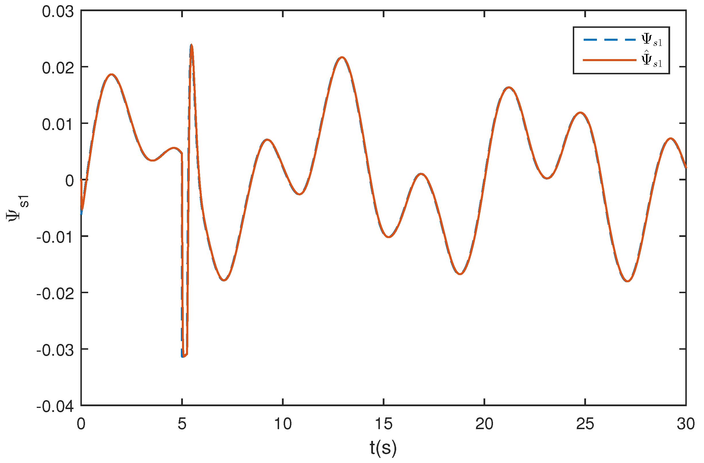
3.1. Design of Disturbance Observer for the First Subsystem

According to (1), the first subsystem can be written as

$${\dot{x}}_1=f_1(x_1)+g_1(x_1)x_2+\Delta f_1\left(x_1\right)+d_1\left(t\right)$$

(12)

In (12), the system uncertainty $\Delta f_1\left(x_1\right)$ and external disturbance $d_1(t)$ are considered simultaneously. In traditional ESO method, $\Delta f_1\left(x_1\right)$ and $d_1(t)$ are merged into a single equivalent uncertainty. To improve the disturbance estimation performance, it is necessary to introduce different mechanisms to handle the system uncertainty and the external disturbance separately.

To efficiently tackle the unknown function vector $\Delta f_1\left(x_1\right)$, the RBFNN is employed to approximate it. The approximation output of the RBFNN can be written as

$$\Delta f_1\left(x_1\right)=W_1^{{*}^T}{S}_1\left(J_1\right)+{\iota }_1^{*}$$

(13)

where $J_1=x_1$, $W_1^{{*}^T}={\left[W_{11}^{*},W_{12}^{*}\right]}^T\in R^{2\times p_1}$, $S_1\left(J_1\right)\in R^{p_1}$, ${\iota }_1^{*}\in R^{2\times 1}$.

Substituting (13) into (12), we obtain

$${\dot{x}}_1=f_1(x_1)+g_1(x_1)x_2+W_1^{{*}^T}{S}_1\left(J_1\right)+D_1$$

(14)

where $D_1=d_1\left(t\right)+{\iota }_1^{*}$.

Extending $D_1$ as an additional state variable, i.e., defining $x_3=D_1$, (14) can be rewritten as

$$\begin{array}{ccc}\hfill {\dot{x}}_1& =& f_1(x_1)+g_1(x_1)x_2+W_1^{{*}^T}{S}_1\left(J_1\right)+x_3\hfill \\ \hfill {\dot{x}}_3& =& {\hslash }_1\left(t\right)\hfill \end{array}$$

(15)

where $x_3={\left[x_{31},x_{32}\right]}^T$; ${\hslash }_1={\left[{\hslash }_{11},{\hslash }_{12}\right]}^{\mathrm{T}}$ is an unknown bounded time derivative function vector of $D_1$.

According to the structure of extended system (15), a linear ESO combined with the RBFNN can be constructed as

$$\begin{array}{ccc}\hfill {\dot{\widehat{x}}}_1& =& f_1(x_1)+g_1(x_1)x_2+{\widehat{W}}_1^T{S}_1\left(J_1\right)+{\widehat{x}}_3-l_{1s}{\tilde{x}}_1\hfill \\ \hfill {\dot{\widehat{x}}}_3& =& -l_{2s}{\tilde{x}}_1\hfill \end{array}$$

(16)

where ${\widehat{x}}_1,{\widehat{x}}_3$ are the states of the observer (16); ${\widehat{x}}_1$ is the estimation of $x_1$; ${\widehat{W}}_1^T={\left[{\widehat{W}}_{11},{\widehat{W}}_{12}\right]}^T\in R^{2\times p_1}$ is the estimation of $W_1^{*}$; ${\widehat{x}}_3$ is the estimation of $x_3$; ${\tilde{x}}_1={\widehat{x}}_1-x_1$; And $l_{1s}=diag\{l_{1s1},l_{1s2}\}>0$, $l_{2s}=diag\{l_{2s1},l_{2s2}\}>0$ are design matrixes.

Invoking (15) and (16), we obtain

$$\begin{array}{ccc}\hfill {\dot{\tilde{x}}}_1& =& {\tilde{W}}_1^T{S}_1\left(J_1\right)+{\tilde{x}}_3-l_{1s}{\tilde{x}}_1\hfill \\ \hfill {\dot{\tilde{x}}}_3& =& -l_{2s}{\tilde{x}}_1-{\hslash }_1\hfill \end{array}$$

(17)

Define ${\left[{\epsilon }_{11},{\epsilon }_{12}\right]}^T={\left[{\tilde{x}}_{11},{\tilde{x}}_{12}\right]}^T$, ${\left[{\epsilon }_{31},{\epsilon }_{32}\right]}^T={\left[\frac{{\tilde{x}}_{31}}{{\omega }_{11}},\frac{{\tilde{x}}_{32}}{{\omega }_{12}}\right]}^T$. Then (17) can be written as

$$\left[\begin{array}{c}{\dot{\epsilon }}_{1i}\\ {\dot{\epsilon }}_{3i}\end{array}\right]={\omega }_{1i}{A}_{si}\left[\begin{array}{c}{\epsilon }_{1i}\\ {\epsilon }_{3i}\end{array}\right]+B_{si}{\tilde{W}}_{1i}^T{S}_1\left(J_1\right)-C_{si}\frac{{\hslash }_{1i}}{{\omega }_{1i}}i=1,2$$

(18)

where $A_{si}=\left[\begin{array}{cc}\frac{-l_{1si}}{{\omega }_{1i}}& 1\\ \frac{-l_{2si}}{{\omega }_{1i}^2}& 0\end{array}\right]$, $B_{si}=\left[\begin{array}{c}1\\ 0\end{array}\right]$, $C_{si}=\left[\begin{array}{c}0\\ 1\end{array}\right]$; And ${\omega }_{1i}>0,i=1,2$ is a design constant.

Hence, it can be easily proved that $A_{si}$ is Hurwitz, if $l_{1si}=2k_{si}{\omega }_{1i}$, $l_{2si}=k_{si}^2{\omega }_{1i}^2,i=1,2$, and $k_{si}$ is a positive constant. Thus, there exists a positive definite matrix $P_{si},i=1,2$ satisfying the following Lyapunov equation:

$$A_{si}^T{P}_{si}+P_{si}{A}_{si}=-2I$$

(19)

In this subsection, the disturbance observer (16) for the first subsystem (12) has been proposed. Selecting the parameters of (16) by the given method, $A_{si}$ has been proved to be Hurwitz. And the positive definite matrix $P_{si},i=1,2$ will be used in the design of the Lyapunov function (38), which is very important in the stability analysis of the proposed observer (16) and the closed-loop system.

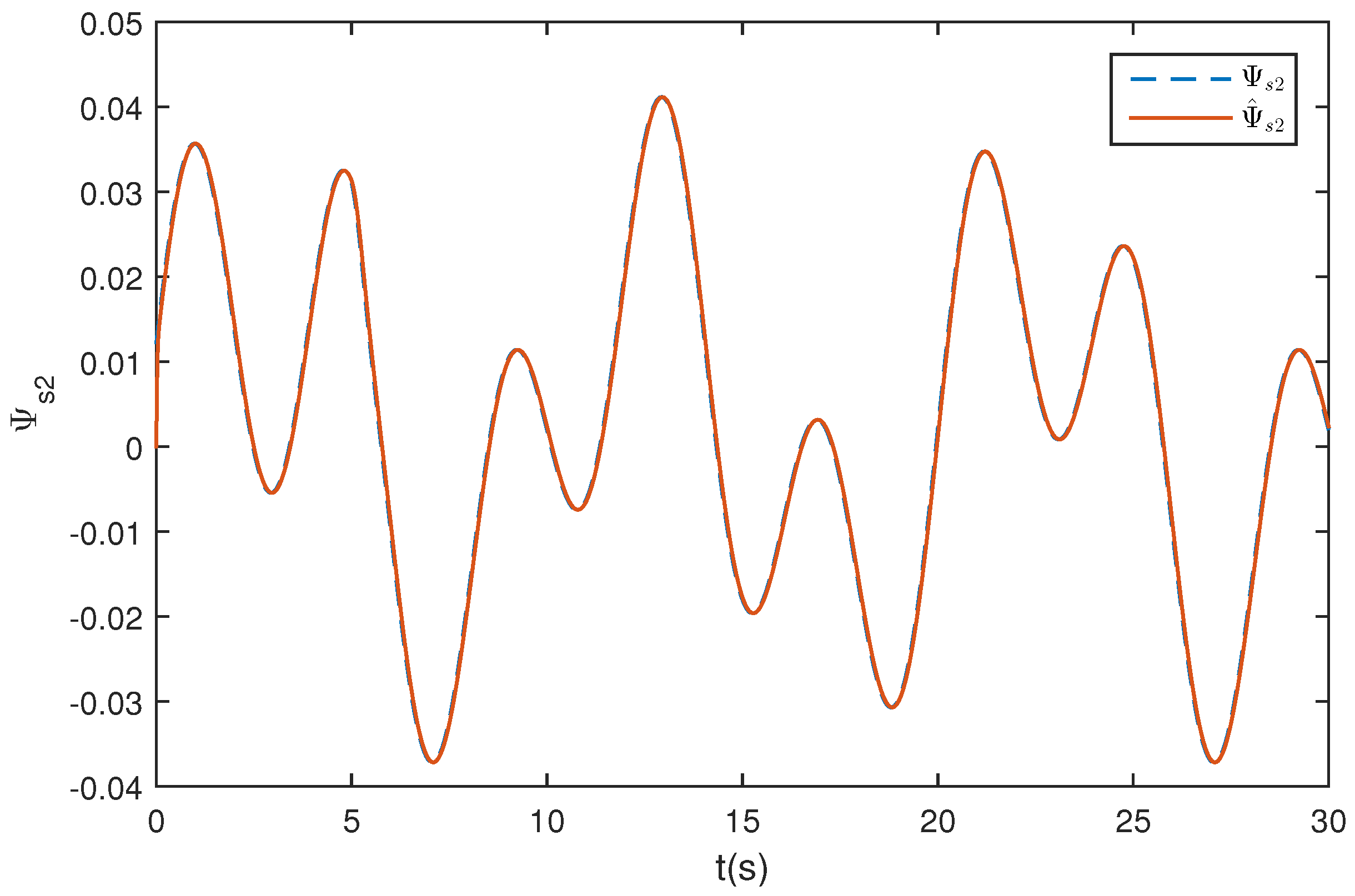
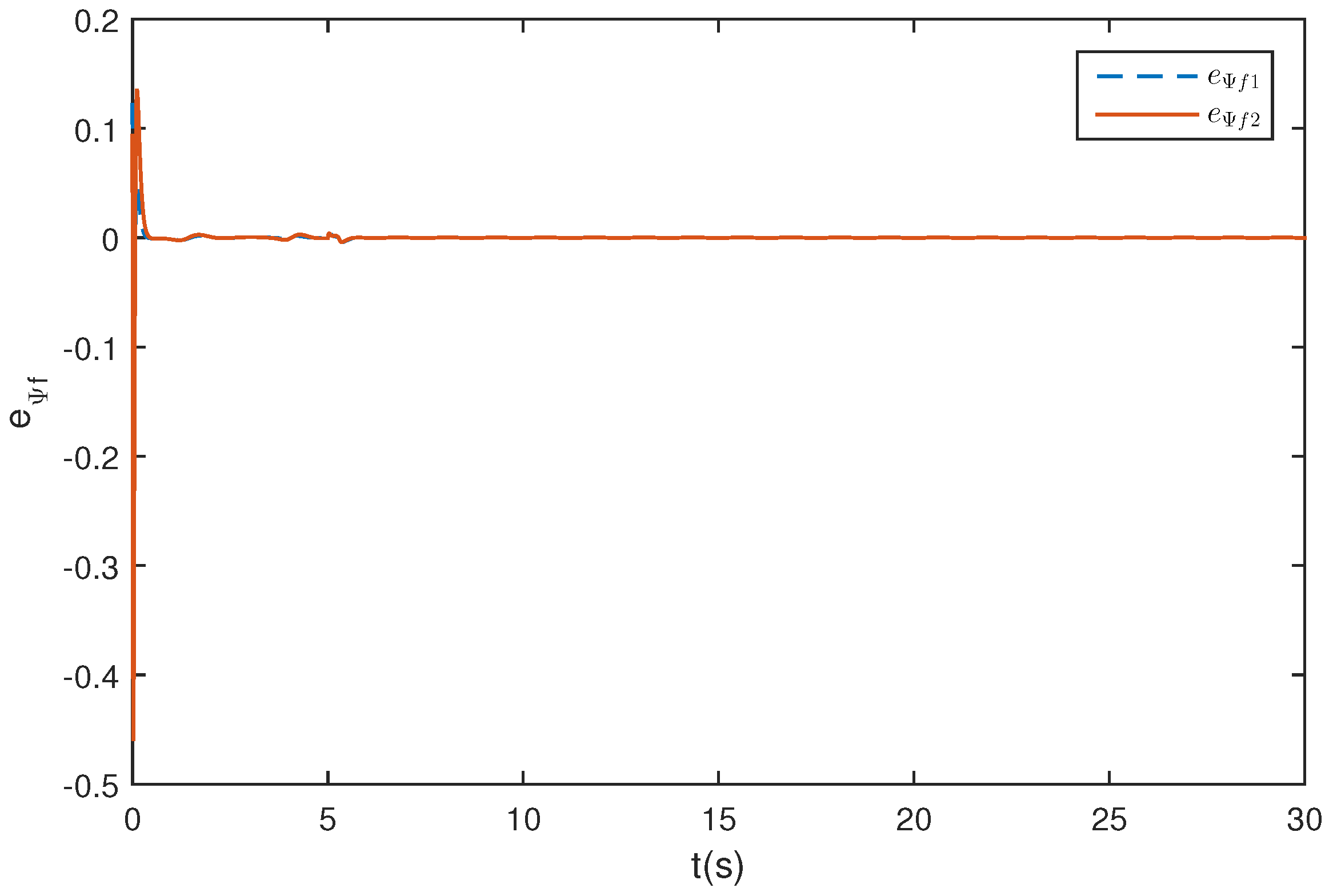
3.2. Design of Disturbance Observer for the Second Subsystem

According to (1), the second subsystem can be written as

$${\dot{x}}_2=f_2(x_1,x_2)+g_2(x_1,x_2)u(v)+\Delta f_2(x_1,x_2)+G_2^{\prime }{h}_2+d_2\left(t\right)$$

(20)

It is more complicated that multiple disturbances are considered in (20). $\Delta f_2(x_1,x_2)$ is the unmodeled system uncertainty, which is an unknown function of the system states. $h_2$ is the unmeasurable unsteady moment aerodynamic coefficient vector whose model can be achieved by wind tunnel experiments. And $d_2(t)$ represents the external disturbance. Similarly, different mechanisms are adopted to handle these different disturbances in this section. Meanwhile, to improve the disturbance estimation performance, the model information of the unmeasurable unsteady moment aerodynamic coefficient vector $h_2$ is fully utilized.

Invoking (2) and (20), the augmented second subsystem state equations can be written as

$$\begin{array}{ccc}\hfill {\dot{x}}_2& =& f_2(x_1,x_2)+g_2(x_1,x_2)u(v)+\Delta f_2(x_1,x_2)+G_2^{\prime }{h}_2+d_2\left(t\right)\hfill \\ \hfill {\dot{h}}_2& =& -B_2\left(\beta \right)h_2-A_2\left(\beta \right){\dot{x}}_1\hfill \end{array}$$

(21)

where $G_2^{\prime }=diag\left\{G_{21},G_{22}\right\}$, and $G_{21}>0$, $G_{22}>0$ are constants.

Similar to (13), considering the neural network approximation of $\Delta f_2(x_1,x_2)$, (21) can be written as

$$\begin{array}{ccc}\hfill {\dot{x}}_2& =& f_2(x_1,x_2)+g_2(x_1,x_2)u(v)+W_2^{{*}^T}{S}_2\left(J_2\right)+G_2^{\prime }{h}_2+D_2\hfill \\ \hfill {\dot{h}}_2& =& -B_2\left(\beta \right)h_2-A_2\left(\beta \right){\dot{x}}_1\hfill \end{array}$$

(22)

where $D_2=d_2\left(t\right)+{\iota }_2^{*}$, $\Delta f_2\left(x_1,x_2\right)=W_2^{{*}^T}{S}_2\left(J_2\right)+{\iota }_2^{*}$. $J_2={[x_1^T,x_2^T]}^T$, $W_2^{{*}^T}={\left[W_{21}^{*},W_{22}^{*}\right]}^T\in R^{2\times p_2}$, $S_2\left(J_2\right)\in R^{p_2}$, ${\iota }_2^{*}\in R^{2\times 1}$.

Defining $x_4=G_2^{\prime }{h}_2+D_2$ and invoking (14), the time derivative of $x_4$ is given by

$$\begin{array}{ccc}\hfill {\dot{x}}_4& =& {G^{\prime }}_2{\dot{h}}_2+{\dot{D}}_2\hfill \\ & =& {G^{\prime }}_2\left(-B_2\left(\beta \right)h_2-A_2\left(\beta \right)\left(f_1(x_1)+g_1(x_1)x_2+W_1^{{*}^T}{S}_1\left(J_1\right)+D_1\right)\right)+{\dot{D}}_2\hfill \\ & =& -B_2\left(\beta \right)x_4-{G^{\prime }}_2{A}_2\left(\beta \right)\left(f_1(x_1)+g_1(x_1)x_2\right)-{G^{\prime }}_2{A}_2\left(\beta \right)W_1^{{*}^T}{S}_1\left(J_1\right)\hfill \\ & & -{G^{\prime }}_2{A}_2\left(\beta \right)D_1+B_2\left(\beta \right)D_2+{\dot{D}}_2\hfill \\ & =& -B_2\left(\beta \right)x_4-{G^{\prime }}_2{A}_2\left(\beta \right)\left(f_1(x_1)+g_1(x_1)x_2\right)-{G^{\prime }}_2{A}_2\left(\beta \right)W_1^{{*}^T}{S}_1\left(J_1\right)+x_5\hfill \end{array}$$

(23)

where $x_5=-G_2^{\prime }{A}_2\left(\beta \right)D_1+B_2\left(\beta \right)D_2+{\dot{D}}_2$ .

Then, invoking (23), the extended system of (22) can be written as

$$\begin{array}{ccc}\hfill {\dot{x}}_2& =& f_2(x_1,x_2)+g_2(x_1,x_2)u(v)+W_2^{{*}^T}{S}_2\left(J_2\right)+x_4\hfill \\ \hfill {\dot{x}}_4& =& -B_2\left(\beta \right)x_4-G_2^{\prime }{A}_2\left(\beta \right)\left(f_1(x_1)+g_1(x_1)x_2\right)-G_2^{\prime }{A}_2\left(\beta \right)W_1^{{*}^T}{S}_1\left(J_1\right)+x_5\hfill \\ \hfill {\dot{x}}_5& =& {\hslash }_2\left(t\right)\hfill \end{array}$$

(24)

where ${\hslash }_2={\left[{\hslash }_{21},{\hslash }_{22}\right]}^T$ is an unknown bounded time derivative function vector of $x_5$.

Then, a linear type of the ESO can be constructed as

$$\begin{array}{ccc}\hfill {\dot{\widehat{x}}}_2& =& f_2(x_1,x_2)+g_2(x_1,x_2)v+{\widehat{W}}_2^T{S}_2\left(J_2\right)+{\widehat{x}}_4-l_{3f}{\tilde{x}}_2\hfill \\ \hfill {\dot{\widehat{x}}}_4& =& -B_2\left(\beta \right){\widehat{x}}_4-G_2^{\prime }{A}_2\left(\beta \right)\left(f_1(x_1)+g_1(x_1)x_2\right)-G_2^{\prime }{A}_2\left(\beta \right){\widehat{W}}_1^T{S}_1\left(J_1\right)+{\widehat{x}}_5-l_{4f}{\tilde{x}}_2\hfill \\ \hfill {\dot{\widehat{x}}}_5& =& -l_{5f}{\tilde{x}}_2\hfill \end{array}$$

(25)

where ${\widehat{x}}_2$ is the estimation of $x_2$; ${\widehat{x}}_4$ is the estimation of $x_4$; ${\widehat{x}}_5$ is the estimation of $x_5$; ${\widehat{W}}_2^T={\left[{\widehat{W}}_{21},{\widehat{W}}_{22}\right]}^T\in R^{2\times p_2}$ is the estimation of $W_2^{{*}^T}$; ${\tilde{x}}_2={\widehat{x}}_2-x_2$; And $l_{3f}=diag\left\{l_{3f1},l_{3f2}\right\}>0$, $l_{4f}=diag\left\{l_{4f1},l_{4f2}\right\}>0$, $l_{5f}=diag\left\{l_{5f1},l_{5f2}\right\}>0$ are design matrixes.

Invoking (24) and (25), we have

$$\begin{array}{ccc}\hfill {\dot{\tilde{x}}}_2& =& {\tilde{W}}_2^T{S}_2\left(J_2\right)+{\tilde{x}}_4-l_{3f}{\tilde{x}}_2\hfill \\ \hfill {\dot{\tilde{x}}}_4& =& -B_2\left(\beta \right){\tilde{x}}_4-G_2^{\prime }{A}_2\left(\beta \right){\tilde{W}}_1^T{S}_1\left(J_1\right)+{\tilde{x}}_5-l_{4f}{\tilde{x}}_2\hfill \\ \hfill {\dot{\tilde{x}}}_5& =& -l_{5f}{\tilde{x}}_2-{\hslash }_2\left(t\right)\hfill \end{array}$$

(26)

Defining ${\left[{\epsilon }_{21},{\epsilon }_{22}\right]}^T={\left[{\tilde{x}}_{21},{\tilde{x}}_{22}\right]}^T$, ${\left[{\epsilon }_{41},{\epsilon }_{42}\right]}^T={\left[\frac{{\tilde{x}}_{41}}{{\omega }_{21}},\frac{{\tilde{x}}_{42}}{{\omega }_{22}}\right]}^T$, ${\left[{\epsilon }_{51},{\epsilon }_{52}\right]}^T={\left[\frac{{\tilde{x}}_{51}}{{\omega }_{21}^2},\frac{{\tilde{x}}_{52}}{{\omega }_{22}^2}\right]}^T$, we have

$$\left[\begin{array}{c}{\dot{\epsilon }}_{2i}\\ {\dot{\epsilon }}_{4i}\\ {\dot{\epsilon }}_{5i}\end{array}\right]={\omega }_{2i}{A}_{fi}\left[\begin{array}{c}{\epsilon }_{2i}\\ {\epsilon }_{4i}\\ {\epsilon }_{5i}\end{array}\right]+B_{1fi}{\tilde{W}}_{2i}^T{S}_2\left(J_2\right)-B_{2fi}\frac{1}{{\omega }_{2i}}{G}_{2i}{a}_{2i}\left(\beta \right){\tilde{W}}_{11}^T{S}_1\left(J_1\right)-B_{3fi}\frac{1}{{\omega }_{2i}^2}{\hslash }_{2i}\left(t\right)$$

(27)

where $A_{fi}=\left[\begin{array}{ccc}\frac{-l_{3fi}}{{\omega }_{2i}}& 1& 0\\ \frac{-l_{4fi}}{{\omega }_{2i}^2}& \frac{-b_{2i}}{{\omega }_{2i}}& 1\\ \frac{-l_{5fi}}{{\omega }_{2i}^3}& 0& 0\end{array}\right]$, $B_{1fi}=\left[\begin{array}{c}1\\ 0\\ 0\end{array}\right]$, $B_{2fi}=\left[\begin{array}{c}0\\ 1\\ 0\end{array}\right]$, $B_{3fi}=\left[\begin{array}{c}0\\ 0\\ 1\end{array}\right],i=1,2$; ${\omega }_{2i}>0$ is a design constant.

According to the Routh-Hurwitz criterion, it can be easily proved that if the parameters of (25) can be chosen as $\left[l_{3f1},l_{3f2}\right]=\left[3k_{f1}{\omega }_{21},3k_{f2}{\omega }_{22}\right]$, $\left[l_{4f1},l_{4f2}\right]=\left[3k_{f1}^2{\omega }_{21}^2,3k_{f2}^2{\omega }_{22}^2\right]$, $\left[l_{5f1},l_{5f2}\right]=\left[k_{f1}^3{\omega }_{21}^3,k_{f2}^3{\omega }_{22}^3\right]$, and $k_{f1}>0$, $k_{f2}>0$ are design constants, $A_{fi}$ will be Hurwitz. Thus, there exists a positive definite matrix $P_{fi},i=1,2$ satisfying the following Lyapunov equation:

$$A_{fi}^T{P}_{fi}+P_{fi}{A}_{fi}=-2I$$

(28)

In this subsection, the disturbance observer (25) for the second subsystem (20) has been proposed. Selecting the parameters of (25) by the given method, $A_{fi}$ has been proved to be Hurwitz. And the positive definite matrix $P_{fi},i=1,2$ will be used in the design of the Lyapunov function (44), which is very important in the stability analysis of the proposed observer (25) and the closed-loop system.

Now, we have illustrated the design process of disturbance observers (16) and (25). However, according to (18) and (27), we still can’t prove their stability due to the coupling between the observers and the RBFNN which will be design later. Hence, the stability of the disturbance observers will be proved in the stability analysis of the closed-loop system.

4. Design of Robust Backstepping Attitude Control Based on Disturbance Observer

At high AOA, the aerodynamic characteristics of the flow field around an aircraft is quite complicated. Any small changes of the attitude of an aircraft may cause drastic changes of the aerodynamic force and aerodynamic moment, which will severely degrade the aircraft flight performance. Hence, the robust backstepping attitude tracking control law should be further developed for the aircraft at high AOA. To compensate for the matched and unmatched disturbances, the ESOs proposed in Section 3 are employed to estimate them. And the disturbance estimations will be introduced into the design of the virtual control law and the practical control law.

Invoking (15) and (24), the system (1) can be written as

$$\begin{array}{ccc}\hfill {\dot{x}}_1& =& f_1(x_1)+g_1(x_1)x_2+W_1^{{*}^T}{S}_1\left(J_1\right)+x_3\hfill \\ \hfill {\dot{x}}_2& =& f_2(x_1,x_2)+g_2(x_1,x_2)u(v)+W_2^{{*}^T}{S}_2\left(J_2\right)+x_4\hfill \end{array}$$

(29)

Considering the input saturation problem, the following auxiliary system is constructed:

$$\begin{array}{ccc}\hfill {\dot{\xi }}_1& =& g_1\left(x_1\right){\xi }_2-k_{aux1}{\xi }_1\hfill \\ \hfill {\dot{\xi }}_2& =& -k_{aux2}{\xi }_2+g_2\left(x_1,x_2\right)\Delta u\hfill \end{array}$$

(30)

where ${\xi }_1,{\xi }_2\in R^{2\times 1}$; $\Delta u=u(v)-v$; $k_{aux1}=k_{aux1}^T>0$, $k_{aux2}=k_{aux2}^T>0$ are design matrixes.

Considering the backstepping control law design method, we define

$$\begin{array}{ccc}\hfill e_1& =& x_1-y_d-{\xi }_1\hfill \\ \hfill e_2& =& x_2-x_{2c}-{\xi }_2\hfill \end{array}$$

(31)

where $x_{2c}$ is the virtual control law which will be designed later.

In the following, we consider the robust backstepping attitude control design for the wing-rock motion. In the attitude control design, the adaptive RBFNN and the ESO are combined, and the detailed design process is appended as follows.

Step 1: Considering the first equation in (29) and differentiating $e_1$ with respect to time yields

$$\begin{array}{ccc}\hfill {\dot{e}}_1& =& {\dot{x}}_1-{\dot{y}}_d-{\dot{\xi }}_1\hfill \\ & =& f_1(x_1)+g_1(x_1)x_2+W_1^{{*}^T}{S}_1\left(J_1\right)+x_3-{\dot{y}}_d-g_1\left(x_1\right){\xi }_2+k_{aux1}{\xi }_1\hfill \\ & =& f_1(x_1)+g_1(x_1)\left(e_2+x_{2c}+{\xi }_2\right)+W_1^{{*}^T}{S}_1\left(J_1\right)+x_3-{\dot{y}}_d-g_1\left(x_1\right){\xi }_2+k_{aux1}{\xi }_1\hfill \\ & =& f_1(x_1)+g_1(x_1)\left(e_2+x_{2c}\right)+W_1^{{*}^T}{S}_1\left(J_1\right)+x_3-{\dot{y}}_d+k_{aux1}{\xi }_1\hfill \end{array}$$

(32)

The ideal virtual control law ${\overline{x}}_{2c}$ for $x_2$ is designed as

$${\overline{x}}_{2c}=-g_1^{-1}\left(x_1\right)\left[f_1(x_1)+{\widehat{W}}_1^T{S}_1\left(J_1\right)+{\widehat{x}}_3-{\dot{y}}_d+c_1{e}_1+k_{aux1}{\xi }_1\right]$$

(33)

where $c_1=c_1^T>0$ is a matrix to be designed.

And the weight value of RBFNN is updated by

$${\dot{\widehat{W}}}_1={\mathrm{\Lambda }}_1\left(S_1\left(J_1\right)e_1^T-{\rho }_1{\widehat{W}}_1\right)$$

(34)

where ${\mathrm{\Lambda }}_1={\mathrm{\Lambda }}_1^T>0$, ${\rho }_1>0$ are the design parameters.

The dynamic surface control (DSC) technique technique is adopted to obtain the approximation of the time derivative of $x_{2c}$. Introducing a first-order filter with time constant ${\mathrm{\Gamma }}_1=diag\left\{{\tau }_{11},{\tau }_{12}\right\}$, and passing ${\overline{x}}_{2c}$ through it yields

$${\mathrm{\Gamma }}_1{\dot{x}}_{2c}+x_{2c}={\overline{x}}_{2c}{x}_{2c}(0)={\overline{x}}_{2c}(0)$$

(35)

Defining ${\epsilon }_{f1}=x_{2c}-{\overline{x}}_{2c}$ and invoking Equation (35), we have

$$\begin{array}{ccc}\hfill {\dot{\epsilon }}_{f1}& =& {\dot{x}}_{2c}-{\dot{\overline{x}}}_{2c}\hfill \\ & =& -{\mathrm{\Gamma }}_1^{-1}{\epsilon }_{f1}+\left[-\frac{\partial {\overline{x}}_{2c}}{\partial x_1}{\dot{x}}_1-\frac{\partial {\overline{x}}_{2c}}{\partial {\widehat{W}}_1}{\dot{\widehat{W}}}_1-\frac{\partial {\overline{x}}_{2c}}{\partial {\widehat{x}}_3}{\dot{\widehat{x}}}_3-\frac{\partial {\overline{x}}_{2c}}{\partial y_d}{\dot{y}}_d-\frac{\partial {\overline{x}}_{2c}}{\partial {\dot{y}}_d}{\ddot{y}}_d-\frac{\partial {\overline{x}}_{2c}}{\partial {\xi }_1}{\dot{\xi }}_1\right]\hfill \\ & =& -{\mathrm{\Gamma }}_1^{-1}{\epsilon }_{f1}+M_1(x_1,{\widehat{W}}_1,{\widehat{x}}_3,{\xi }_1,{\xi }_2,y_d,{\dot{y}}_d,{\ddot{y}}_d)\hfill \\ & =& -{\mathrm{\Gamma }}_1^{-1}{\epsilon }_{f1}+M_1\left(•\right)\hfill \end{array}$$

(36)

where $M_1(•)$ is the sufficiently smooth function vector about ${\mathrm{\Pi }}_0$ and ${\mathrm{\Pi }}_1:(x_1,{\widehat{W}}_1,{\widehat{x}}_3,{\xi }_1,{\xi }_2)$. Since the set ${\mathrm{\Pi }}_0$ and ${\mathrm{\Pi }}_1$ are compacts, ${\mathrm{\Pi }}_0\times {\mathrm{\Pi }}_1$ is also compact. Therefore, $M_1(•)$ has a maximum ${\overline{M}}_1$ on ${\mathrm{\Pi }}_0\times {\mathrm{\Pi }}_1$.

Then, we have

$${\dot{\epsilon }}_{f1}\le -{\mathrm{\Gamma }}_1^{-1}{\epsilon }_{f1}+{\overline{M}}_1$$

(37)

Choose the Lyapunov function candidate as

$$V_1=\frac{1}{2}{e}_1^T{e}_1+\frac{1}{2}{\epsilon }_{f1}^T{\epsilon }_{f1}+\frac{1}{2}{\displaystyle \sum _{i=1}^2}\left[{\epsilon }_{1i},{\epsilon }_{3i}\right]P_{si}{\left[{\epsilon }_{1i},{\epsilon }_{3i}\right]}^T+\frac{1}{2}tr\left({\tilde{W}}_1^T{\mathrm{\Lambda }}_1^{-1}{\tilde{W}}_1\right)+\frac{1}{2}{\xi }_1^T{\xi }_1$$

(38)

Define ${\epsilon }_{13i}={\left[{\epsilon }_{1i},{\epsilon }_{3i}\right]}^T$, then the time derivative of $V_1$ can be written as

$$\begin{array}{ccc}\hfill {\dot{V}}_1& \le & e_1^T{g}_1(x_1)e_2-\left(c_1-\frac{1}{2}{\overline{\lambda }}_1-max\left\{{\omega }_{1i}\right\}\right)e_1^T{e}_1-\left({\lambda }_{max}\left({\mathrm{\Gamma }}_1^{-1}\right)-1\right){\epsilon }_{f1}^T{\epsilon }_{f1}\hfill \\ & & -\left(\frac{{\rho }_1}{2}-\frac{1}{\tau }\right){∥{\tilde{W}}_1∥}^2+{\displaystyle \sum _{i=1}^2}\left(-\frac{\left(\frac{3}{4}{\omega }_{1i}-\frac{\tau }{2}{M}_{PBS1}^2-\frac{M_{P{C}_{si}}}{4\tau }\right)}{{\lambda }_{max}\left(P_{si}\right)}{\epsilon }_{13i}^T{P}_{si}{\epsilon }_{13i}\right)\hfill \\ & & -{\xi }_1^T{k}_{aux1}{\xi }_1+\frac{1}{2}{\overline{\lambda }}_1{\xi }_1^T{\xi }_1+\frac{1}{2}{\xi }_2^T{\xi }_2+{\displaystyle \sum _{i=1}^2}\left(\frac{M_{P{C}_{si}}\tau }{{\omega }_{1i}^2}{M}_{{\hslash }_{1i}}^2\right)+\frac{1}{2}{\overline{M}}_1^2+\frac{{\rho }_1}{2}{∥W_1^{*}∥}^2\hfill \end{array}$$

(39)

where $∥P_{si}{C}_{si}∥=M_{P{C}_{si}}$, $∥{\hslash }_{1i}∥\le M_{{\hslash }_{1i}}$, $∥P_{si}{B}_{si}∥∥S_1\left(J_1\right)∥\le M_{PBS1}$, and $\tau >0$ is a design constant.

The detailed analysis of the time derivative of $V_1$ is shown in Appendix A.

Step 2: Invoking (29), differentiating $e_2$ yields

$$\begin{array}{ccc}\hfill {\dot{e}}_2& =& {\dot{x}}_2-{\dot{x}}_{2c}-{\dot{\xi }}_2\hfill \\ & =& f_2(x_1,x_2)+g_2(x_1,x_2)u\left(v\right)+W_2^{{*}^T}{S}_2\left(J_2\right)+x_4-{\dot{x}}_{2c}+k_{aux2}{\xi }_2-g_2\left(x_1,x_2\right)\Delta u\hfill \\ & =& f_2(x_1,x_2)+g_2(x_1,x_2)v+W_2^{{*}^T}{S}_2\left(J_2\right)+x_4-{\dot{x}}_{2c}+k_{aux2}{\xi }_2\hfill \end{array}$$

(40)

The control law v is designed as

$$v=-g_2^{-1}(x_1,x_2)\left(f_2(x_1,x_2)+{\widehat{W}}_2^T{S}_2\left(J_2\right)+{\widehat{x}}_4-{\dot{x}}_{2c}+c_2{e}_2+g_1^T\left(x_1\right)e_1+k_{aux2}{\xi }_2\right)$$

(41)

where $c_2=c_2^T>0$ is a design matrix, and ${\widehat{W}}_2$ is updated by

$${\dot{\widehat{W}}}_2={\mathrm{\Lambda }}_2\left(S_2\left(J_2\right)e_2^T-{\rho }_2{\widehat{W}}_2\right)$$

(42)

where ${\rho }_2>0$, ${\mathrm{\Lambda }}_2={\mathrm{\Lambda }}_2^T>0$ are design parameters.

Substituting the controller v into Equation (40), we obtain

$${\dot{e}}_2=-g_1^T\left(x_1\right)e_1-{\tilde{W}}_2^T{S}_2\left(J_2\right)-{\tilde{x}}_4-c_2{e}_2$$

(43)

where ${\tilde{W}}_2={\widehat{W}}_2-W_2^{*}$, ${\tilde{x}}_4={\widehat{x}}_4-x_4$ are the estimation errors.

Define ${\epsilon }_{245i}={\left[{\epsilon }_{2i},{\epsilon }_{4i},{\epsilon }_{5i}\right]}^T,i=1,2$, and consider the Lyapunov function candidate as

$$V_2=\frac{1}{2}{e}_2^T{e}_2+\frac{1}{2}{\displaystyle \sum _{i=1}^2}{\epsilon }_{245i}^T{P}_{fi}{\epsilon }_{245i}+\frac{1}{2}tr\left({\tilde{W}}_2^T{\mathrm{\Lambda }}_2^{-1}{\tilde{W}}_2\right)+\frac{1}{2}{\xi }_2^T{\xi }_2$$

(44)

The time derivative of $V_2$ is given by

$$\begin{array}{ccc}\hfill {\dot{V}}_2& \le & -e_2^T{g}_1^T\left(x_1\right)e_1-\left(c_2-max\left\{{\omega }_{2i}\right\}\right)e_2^T{e}_2-\left(\frac{{\rho }_2}{2}-\frac{1}{\tau }\right){∥{\tilde{W}}_2∥}^2\hfill \\ & & +{\displaystyle \sum _{i=1}^2}\left(-\frac{\left({\omega }_{2i}-\frac{{\omega }_{2i}}{4}-\frac{\tau }{2}{M}_{PBS2}^2-\frac{\tau }{2{\omega }_{2i}^2}{M}_{PBASi}^2-\frac{M_{P{B}_{fi}}}{4\tau }\right)}{{\lambda }_{max}\left(P_{fi}\right)}{\epsilon }_{245i}^T{P}_{fi}{\epsilon }_{245i}\right)\hfill \\ & & +\frac{1}{\tau }{∥{\tilde{W}}_1∥}^2-{\xi }_2^T{k}_{aux2}{\xi }_2+\frac{1}{2}{\overline{\lambda }}_2{\xi }_2^T{\xi }_2+\frac{1}{2}\Delta u^T\Delta u\hfill \\ & & +{\displaystyle \sum _{i=1}^2}\left(\frac{M_{P{B}_{fi}}\tau }{{\omega }_{2i}^4}{M}_{{\hslash }_{2i}}^2\right)+\frac{{\rho }_2}{2}{∥W_2^{*}∥}^2\hfill \end{array}$$

(45)

where $∥P_{fi}{B}_{1fi}∥∥S_2\left(J_2\right)∥\le M_{PBS2}$, $∥P_{fi}{B}_{2fi}{G}_{2i}{a}_{2i}\left(\beta \right)∥∥S_1\left(J_1\right)∥\le M_{PBASi}$, $∥P_{fi}{B}_{3fi}∥\le M_{P{B}_{fi}}$, $∥{\hslash }_{2i}∥\le M_{{\hslash }_{2i}}$.

The detailed analysis of the time derivative of $V_2$ is shown in Appendix B.

Then, the above robust backstepping wing rock control design procedure can be summarized in the following theorem.

Theorem 1.

Considering the nonlinear MIMO lateral model (1) in the presence of unsteady aerodynamics disturbances, external disturbances, system uncertainties, and input saturation, the disturbance observers are designed as (16), (25), the auxiliary system is designed as (30), the filter is designed as (35), and the robust backstepping attitude control law is proposed as (41). Then, the attitude tracking error is convergent and bounded under the proposed adaptive robust backstepping control scheme.

Proof. 

To analyze the stability of the closed-loop system, the following Lyapunov function candidate is chosen as

$$V=V_1+V_2$$

(46)

Then, differentiating V and invoking Equations (39), (45), we have

$$\begin{array}{ccc}\hfill \dot{V}& =& {\dot{V}}_1+{\dot{V}}_2\hfill \\ & =& -\left(c_1-\frac{1}{2}{\overline{\lambda }}_1-max\left\{{\omega }_{1i}\right\}\right)e_1^T{e}_1-\left({\lambda }_{max}\left({\mathrm{\Gamma }}_1^{-1}\right)-1\right){\epsilon }_{f1}^T{\epsilon }_{f1}\hfill \\ & & -\left(\frac{{\rho }_1}{2}-\frac{2}{\tau }\right){∥{\tilde{W}}_1∥}^2+{\displaystyle \sum _{i=1}^2}\left(-\frac{\left(\frac{3}{4}{\omega }_{1i}-\frac{\tau }{2}{M}_{PBS1}^2-\frac{M_{P{C}_{si}}}{4\tau }\right)}{{\lambda }_{max}\left(P_{si}\right)}{\epsilon }_{13i}^T{P}_{si}{\epsilon }_{13i}\right)\hfill \\ & & -\left(c_2-max\left\{{\omega }_{2i}\right\}\right)e_2^T{e}_2-\left(\frac{{\rho }_2}{2}-\frac{1}{\tau }\right){∥{\tilde{W}}_2∥}^2\hfill \\ & & +{\displaystyle \sum _{i=1}^2}\left(-\frac{\left(\frac{3}{4}{\omega }_{2i}-\frac{\tau }{2}{M}_{PBS2}^2-\frac{\tau }{2{\omega }_{2i}^2}{M}_{PBASi}^2-\frac{M_{P{B}_{fi}}}{4\tau }\right)}{{\lambda }_{max}\left(P_{fi}\right)}{\epsilon }_{245i}^T{P}_{fi}{\epsilon }_{245i}\right)\hfill \\ & & -\left({\lambda }_{min}\left(k_{aux1}\right)-\frac{1}{2}{\overline{\lambda }}_1\right){\xi }_1^T{\xi }_1-\left({\lambda }_{min}\left(k_{aux2}\right)-\frac{1}{2}{\overline{\lambda }}_2-\frac{1}{2}\right){\xi }_2^T{\xi }_2\hfill \\ & & +{\displaystyle \sum _{i=1}^2}\left(\frac{M_{P{C}_{si}}\tau }{{\omega }_{1i}^2}{M}_{{\hslash }_{1i}}^2\right)+{\displaystyle \sum _{i=1}^2}\left(\frac{M_{P{B}_{fi}}\tau }{{\omega }_{2i}^4}{M}_{{\hslash }_{2i}}^2\right)+\frac{1}{2}{\overline{M}}_1^2+\frac{{\rho }_1}{2}{∥W_1^{*}∥}^2+\frac{{\rho }_2}{2}{∥W_2^{*}∥}^2+\frac{1}{2}\Delta u^T\Delta u\hfill \\ & \le & -\kappa V+C\hfill \end{array}$$

(47)

where

$$\begin{array}{ccc}\hfill \kappa & =& max\left\{\begin{array}{c}2\left(c_1-\frac{1}{2}{\overline{\lambda }}_1-max\left\{{\omega }_{1i}\right\}\right),2\left({\lambda }_{max}\left({\mathrm{\Gamma }}_1^{-1}\right)-1\right),2\left(\frac{{\rho }_1}{2}-\frac{2}{\tau }\right)\hfill \\ \frac{2\left(\frac{3}{4}{\omega }_{1i}-\frac{\tau }{2}{M}_{PBS1}^2-\frac{M_{P{C}_{si}}}{4\tau }\right)}{{\lambda }_{max}\left(P_{si}\right)},2\left(c_2-max\left\{{\omega }_{2i}\right\}\right),2\left(\frac{{\rho }_2}{2}-\frac{1}{\tau }\right)\hfill \\ \frac{2\left(\frac{3}{4}{\omega }_{2i}-\frac{\tau }{2}{M}_{PBS2}^2-\frac{\tau }{2{\omega }_{2i}^2}{M}_{PBASi}^2-\frac{M_{P{B}_{fi}}}{4\tau }\right)}{{\lambda }_{max}\left(P_{fi}\right)},2\left({\lambda }_{min}\left(k_{aux1}\right)-\frac{1}{2}{\overline{\lambda }}_1\right)\hfill \\ 2\left({\lambda }_{min}\left(k_{aux2}\right)-\frac{1}{2}{\overline{\lambda }}_2-\frac{1}{2}\right)\hfill \end{array}\right\}\hfill \\ \hfill C& =& {\displaystyle \sum _{i=1}^2}\left(\frac{M_{P{C}_{si}}\tau }{{\omega }_{1i}^2}{M}_{{\hslash }_{1i}}^2\right)+{\displaystyle \sum _{i=1}^2}\left(\frac{M_{P{B}_{fi}}\tau }{{\omega }_{2i}^4}{M}_{{\hslash }_{2i}}^2\right)+\frac{1}{2}{\overline{M}}_1^2+\frac{{\rho }_1}{2}{∥W_1^{*}∥}^2+\frac{{\rho }_2}{2}{∥W_2^{*}∥}^2+\frac{1}{2}\Delta u^T\Delta u\hfill \end{array}$$

(48)

According to Equation (47) and Lemma 1, we obtain

$$0\le V\le \frac{C}{\kappa }+\left[V\left(0\right)-\frac{C}{\kappa }\right]e^{-\kappa t}$$

(49)

Considering Equations (31), (46), (49), we obtain

$$\left\{\begin{array}{c}∥e_1∥\le \sqrt{2V}\\ ∥{\xi }_1∥\le \sqrt{2V}\end{array}\right.$$

(50)

Then, we obtain

$$\underset{t\to +\infty }{lim}∥x_1-y_d∥\le \underset{t\to +\infty }{lim}\left(∥x_1-y_d-{\xi }_1∥+∥{\xi }_1∥\right)=2\sqrt{\frac{2C}{\kappa }}$$

(51)

Hence, it is obvious that the attitude tracking error is convergent and bounded under the proposed adaptive robust backstepping control scheme. Similarly, we can conclude that the disturbance estimation errors ${\epsilon }_{13i}$, ${\epsilon }_{245i},i=1,2$ of the disturbance observers (16) and (25) are also convergent and bounded.

This concludes the proof. ☐

5. Simulation Study

In this section, the simulation results are given to verify the effectiveness of the proposed robust control scheme in suppression of wing rock motion at high AOA. In this section, the aircraft model in [40] and the unsteady model in [41] are adopted to demonstrate the attitude control performance and the disturbance rejection performance of the above designed controller.

In simulations, initial conditions for the aircraft are take as $\alpha ={55}^{\circ }$, $x_1\left(0\right)={\left[5^{\circ },0^{\circ }\right]}^T$, $x_2\left(0\right)={\left[0^{\circ }/s,0^{\circ }/s\right],}^T$, whereas initial conditions for the proposed ESO are taken as $\left[{\widehat{x}}_1^T,\left(0\right),{\widehat{x}}_3^T,\left(0\right)\right]$ = [5.7, 0, 0, 0], $\left[{\widehat{x}}_2^T,\left(0\right),{\widehat{x}}_4^T,\left(0\right),{\widehat{x}}_5^T,\left(0\right)\right]$ = [0, 0, 0, 0, 0, 0]. And the initial condition for the auxiliary system is chosen as $\left[{\xi }_1^T,{\xi }_2^T\right]$ = [0, 0, 0, 0]. The time constant for (35) is designed as ${\mathrm{\Gamma }}_1$ = diag {0.08, 0.08}.

It is very important to choose suitable parameters for the ESO. And the observer gains of the error dynamics (18) and (27)are designed by placing the observer error dynamics poles around $\left[-15,-15\right]$ and $\left[-15,-15,-15\right]$, respectively. Hence, $\left[k_{s1},k_{s2}\right]=\left[15,15\right]$, $\left[k_{f1},k_{f2}\right]=\left[15,15\right]$, $\left[{\omega }_{11},{\omega }_{12}\right]=\left[6,6\right]$, $\left[{\omega }_{21},{\omega }_{22}\right]=\left[6,6\right]$. Large $k_{si}$, $k_{fi}$, ${\omega }_{1i}$, ${\omega }_{2i},i=1,2$ will improve the disturbance performance, and make the disturbance estimation errors arbitrarily small. Meanwhile, large $k_{si}$ and $k_{fi}$ will reduce the conservatism of the controller proposed in this paper.

The parameters for the controller (41) are chosen as $\left[c_1^T,c_2^T\right]=\left[6,6,10,10\right]$. Large control parameters $\left[c_1^T,c_2^T\right]$ will improve the control performance and reduce steady-state tracking errors. However, large control parameters will also induce serious input saturation. The parameters for the auxiliary system (30) is designed as $\left[k_{aux1}^T,k_{aux2}^T\right]=\left[6,6,60,60\right]$. The parameters for the adaptive RBFNNs (34) and (42) are chosen as ${\mathrm{\Lambda }}_1=40$, ${\rho }_1=0.5$, ${\mathrm{\Lambda }}_2=1$, ${\rho }_2=0.8$.

In the simulation study, the system uncertainties $\Delta f_1\left(x_1\right)$ and $\Delta f_2\left(x_1,x_2\right)$ are assumed as $+40\%$ variation of the force and moment aerodynamic coefficients. In addition, we assume that the unknown time–varying disturbances imposed on the aircraft are

$$\left[\begin{array}{c}{\dot{h}}_l\\ {\dot{h}}_n\end{array}\right]=-\left[\begin{array}{cc}5& 0\\ 0& 5\end{array}\right]\left[\begin{array}{c}{h}_l\\ h_n\end{array}\right]-\left[\begin{array}{c}-0.02\\ -0.05\end{array}\right]\dot{\beta }$$

(52)

$$d_1=\left[\begin{array}{c}{d}_{11}\\ d_{12}\end{array}\right]=\left[\begin{array}{c}0.01\left(sin\left(0.5\pi t\right)+sin\left(0.2\pi t\right)+0.1\right)\\ 0.02\left(sin\left(0.5\pi t\right)+sin\left(0.2\pi t\right)+0.1\right)\end{array}\right]$$

(53)

$$d_2=\left[\begin{array}{c}{d}_{21}\\ d_{22}\end{array}\right]=\left[\begin{array}{c}0.01\left(sin\left(5t\right)+sin\left(2t\right)+0.3\right)\\ 0.01\left(sin\left(5t\right)+sin\left(2t\right)+0.3\right)\end{array}\right]$$

(54)

According to Figure 1, Figure 2, Figure 3 and Figure 4, the states of the aircraft diverge rapidly when the wing rock motion appears. Hence, it is necessary to adopt appropriate control scheme immediately after the wing rock phenomenon is detected. In the following simulations, we assume that the wing rock motion is detected at 5 s, and then the controller (41) is executed immediately.

To facilitate the description, we define the compounded uncertainties ${\mathrm{\Psi }}_s$, ${\mathrm{\Psi }}_f$ as following

$$\begin{array}{ccc}\hfill {\mathrm{\Psi }}_s& =& {\left[{\mathrm{\Psi }}_{s1},{\mathrm{\Psi }}_{s2}\right]}^T=\Delta f_1\left(x_1\right)+d_1\left(t\right)\hfill \\ \hfill {\mathrm{\Psi }}_f& =& {\left[{\mathrm{\Psi }}_{f1},{\mathrm{\Psi }}_{f2}\right]}^T=\Delta f_2\left(x_1,x_2\right)+G_2^{\prime }{h}_2+d_2\left(t\right)\hfill \end{array}$$

(55)

Meanwhile, we define the two estimation errors $e_{\mathrm{\Psi }s}={\left[e_{\mathrm{\Psi }s1},e_{\mathrm{\Psi }s2}\right]}^T$, $e_{\mathrm{\Psi }f}={\left[e_{\mathrm{\Psi }f1},e_{\mathrm{\Psi }f2}\right]}^T$ as

$$\begin{array}{ccc}\hfill e_{\mathrm{\Psi }s}& =& {\widehat{\mathrm{\Psi }}}_s-{\mathrm{\Psi }}_s={\widehat{W}}_1^T{S}_1\left(J_1\right)+{\widehat{x}}_3-{\mathrm{\Psi }}_s\hfill \\ \hfill e_{\mathrm{\Psi }f}& =& {\widehat{\mathrm{\Psi }}}_f-{\mathrm{\Psi }}_f={\widehat{W}}_2^T{S}_2\left(J_2\right)+{\widehat{x}}_4-{\mathrm{\Psi }}_f\hfill \end{array}$$

(56)

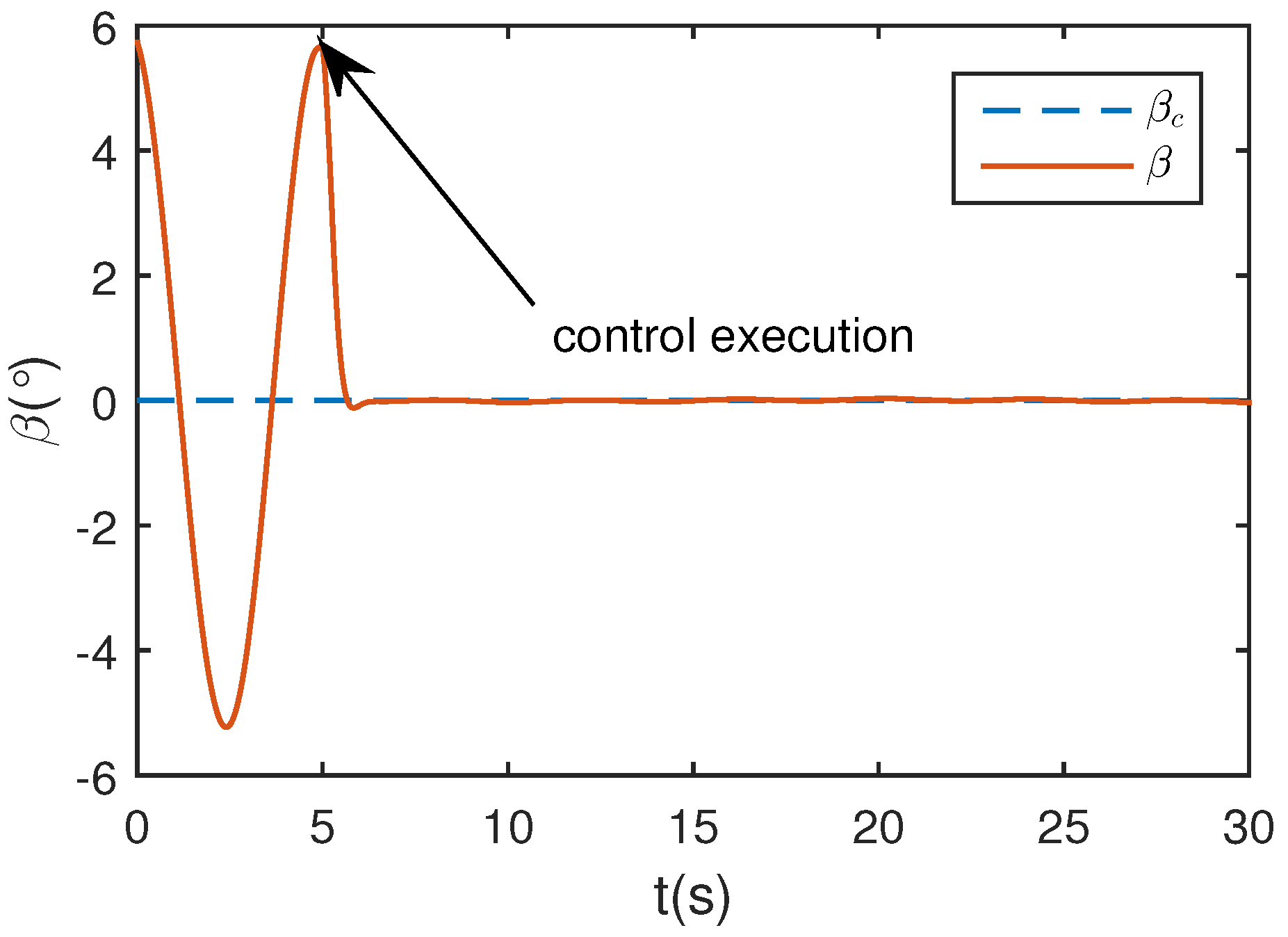
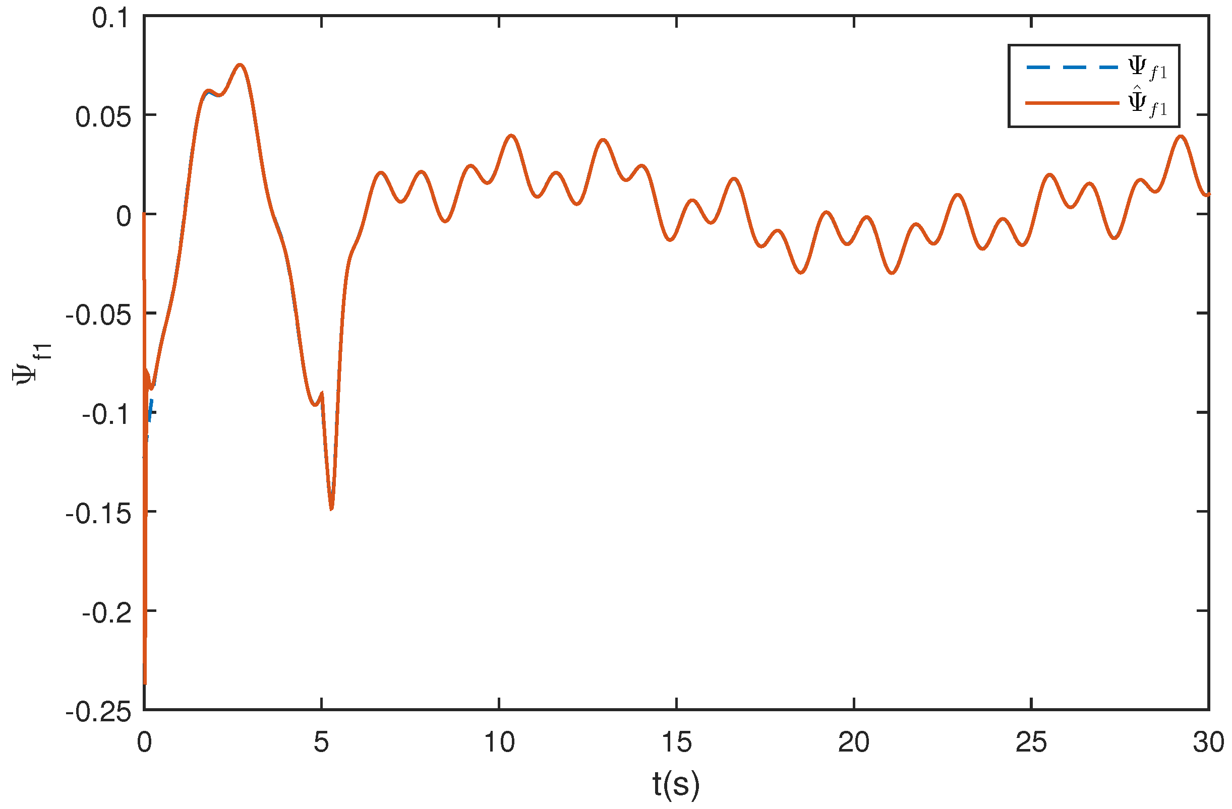
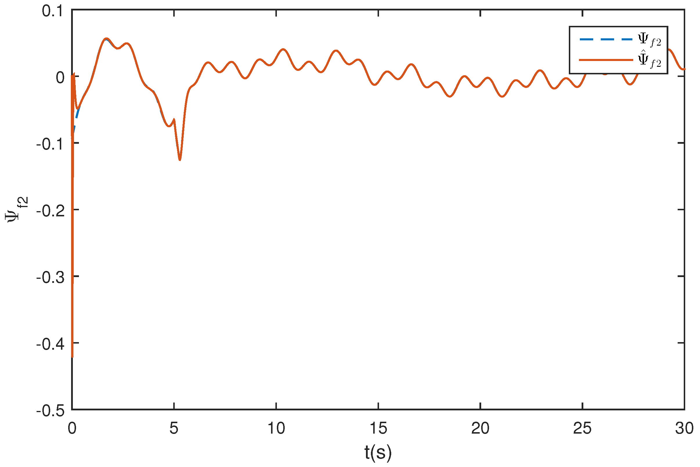
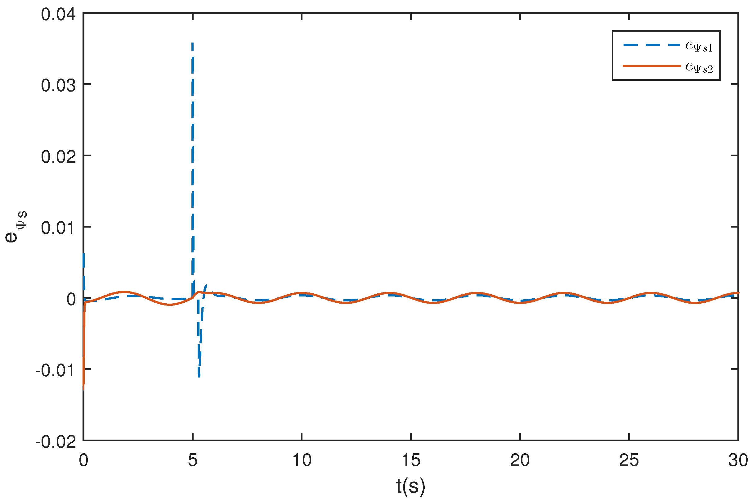
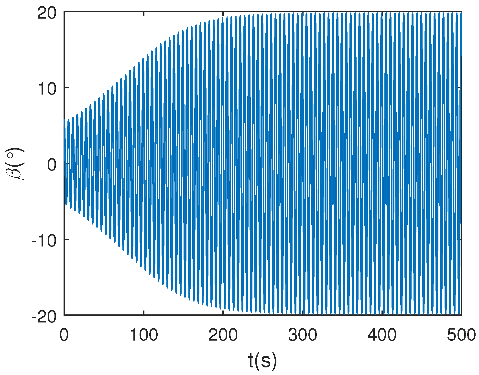
5.1. Wing Rock Control

In this subsection, the control objective is to track a desired attitude command while suppressing the wing-rock motion. The simulations are given by considering a reference attitude angle trajectory as

$$\begin{array}{ccc}\hfill {\beta }_c& =& 0^{\circ }\hfill \\ \hfill {\mu }_c& =& 20sin{\left(0.4\pi t\right)}^{\circ }\hfill \end{array}$$

(57)

The controller is executed at 5 s after the wing-rock motion appears, and the simulation results are presented in Figure 5, Figure 6, Figure 7, Figure 8, Figure 9, Figure 10, Figure 11, Figure 12, Figure 13 and Figure 14.

Figure 5 and Figure 6 show that the wing rock motion appears, and the aircraft starts to oscillate at the beginning. Then, after the controller (41) is executed in the fifth second, the states μ, β converge to the desired attitude command (57) quickly, which means that the controller can achieve satisfactory tracking performance while suppressing the wing rock motion. Figure 7, Figure 8, Figure 9 and Figure 10 show that the ESO can estimate the uncertainty quite accurately. In Figure 7, the compounded disturbance ${\mathrm{\Psi }}_{s1}$ diverged quickly in fifth seconds, and the proposed disturbance observer can still estimate the disturbance well. The estimation errors are plotted in Figure 11 and Figure 12, which show that the proposed disturbance observer not only has good steady-state performance, but also has good transient performance. Meanwhile, the corresponding control input histories are given in Figure 13 and Figure 14, respectively.

From the simulation results, we know that the developed ESO based robust control law is valid for the nonlinear MIMO lateral model of an aircraft with system uncertainty, unsteady aerodynamic disturbance, and input saturation.

One of the focuses of this paper is the robust control of wing rock motion suffering multiple disturbances. To enhance the system robustness, an improved ESO is proposed combined with the RBFNN. Next, the simulation will be carried out to compare the performance of the proposed ESO with existing traditional ESOs.

5.2. Comparison with Traditional ESO

In the traditional ESO design method, all the uncertainties are merged into a single compounded uncertainty. Hence, we rewrite (4) as follows

$$\begin{array}{ccc}\hfill {\dot{x}}_1& =& f_1(x_1)+g_1(x_1)x_2+{\mathrm{\Psi }}_s\hfill \\ \hfill {\dot{x}}_2& =& f_2(x_1,x_2)+g_2(x_1,x_2)u(v)+{\mathrm{\Psi }}_f\hfill \end{array}$$

(58)

Considering that a linear ESO is developed in this paper, the traditional linear ESO (LESO) is considered for comparison instead of traditional nonlinear ESO. Meanwhile, the use of linear ESO offers certain advantages. Firstly, the close loop stability for nonlinear ESO is hard to established conclusively. Secondly, the LESO is easy from hardware implementation point of view.

In [18], the authors have presented the wing rock control law based on the linear ESO. Hence, according to [18], the LESO for (58) is designed as

$$\begin{array}{ccc}\hfill {\dot{\widehat{x}}}_{Ls}& =& f_1(x_1)+g_1(x_1)x_2+{\widehat{\mathrm{\Psi }}}_{sL}-{l^{\prime }}_{Ls1}{e^{\prime }}_{Ls}\hfill \\ \hfill {\dot{\widehat{\mathrm{\Psi }}}}_{sL}& =& -{l^{\prime }}_{Ls2}{e^{\prime }}_{Ls}\hfill \\ \hfill {\dot{\widehat{x}}}_{Lf}& =& f_2(x_1,x_2)+g_2(x_1,x_2)u(v)+{\widehat{\mathrm{\Psi }}}_{fL}-{l^{\prime }}_{Lf1}{e^{\prime }}_{Lf}\hfill \\ \hfill {\dot{\widehat{\mathrm{\Psi }}}}_{fL}& =& -{l^{\prime }}_{Lf2}{e^{\prime }}_{Lf}\hfill \end{array}$$

(59)

where ${\widehat{x}}_{Ls}$ is the estimation of $x_1$; ${\widehat{\mathrm{\Psi }}}_{sL}={\left[{\widehat{\mathrm{\Psi }}}_{sL1},{\widehat{\mathrm{\Psi }}}_{sL2}\right]}^T$ is the estimation of ${\mathrm{\Psi }}_s$; ${e^{\prime }}_{Ls}={\widehat{x}}_{Ls}-x_1$; ${\widehat{x}}_{Lf}$ is the estimation of $x_2$; ${\widehat{\mathrm{\Psi }}}_{fL}={\left[{\widehat{\mathrm{\Psi }}}_{fL1},{\widehat{\mathrm{\Psi }}}_{fL2}\right]}^T$ is the estimation of ${\mathrm{\Psi }}_f$. ${l^{\prime }}_{Ls1}$, ${l^{\prime }}_{Ls2}$, ${l^{\prime }}_{Lf1}$, ${l^{\prime }}_{Lf2}$ are the positive observer gains.

Similar to the developed disturbance observer in this paper, the observer gains are obtained by following the pole placement technique by placing the observer error dynamics poles at $\left[-15,-15\right]$. Hence, ${l^{\prime }}_{Ls1}=30$, ${l^{\prime }}_{Ls2}=225$, ${l^{\prime }}_{Lf1}=30$, ${l^{\prime }}_{Lf2}=225$. And initial conditions for the traditional LESO (59) are taken as $\left[{\widehat{x}}_{Ls}^T\left(0\right),{\widehat{\mathrm{\Psi }}}_s^T\left(0\right)\right]=\left[5.7,0,0,0\right]$, $\left[{\widehat{x}}_{Lf}^T\left(0\right),{\widehat{\mathrm{\Psi }}}_f^T\left(0\right)\right]=\left[0,0,0,0\right]$. The simulations are carried out by tracking the trajectory (57), and the other design parameters are the same as stated earlier. To facilitate the description, we define ${e^{\prime }}_{\mathrm{\Psi }s}={\widehat{\mathrm{\Psi }}}_{sL}-{\mathrm{\Psi }}_s$, ${e^{\prime }}_{\mathrm{\Psi }f}={\widehat{\mathrm{\Psi }}}_{fL}-{\mathrm{\Psi }}_f$.

The estimation output of the LESO (59) is presented in Figure 15, Figure 16, Figure 17 and Figure 18. In (58), all the uncertainties are merged into a single compounded uncertainty, which leads to a larger value of the time derivative of the compounded uncertainty. Hence, obvious estimation errors can be observed in the output of LESO. Comparing Figure 11 and Figure 12 with Figure 19 and Figure 20, it is obvious that the disturbance observer proposed in this paper can achieve better estimation performance under the same conditions. Meanwhile, we can conclude that the developed disturbance observer not only has good steady-state performance, but also has good transient performance.

5.3. Wing Rock Control under Narrow-Band Disturbances

In many classes of applications like active vibration control and active noise control, the broadband and band-limited disturbances have been considered, which can be of narrow band type (simple or multiple) or of broad band type. To make the simulation more realistic, a narrow-band disturbance (NBD) will be considered in the wing rock control. Usually, a common framework is the assumption that the broadband and band-limited disturbances are the results of a white noise or a Dirac impulse passing through the shaping filter. Similar to [47], the transfer function of the shaping filter is taken to be $\frac{s}{s^2+0.95409s+9103}$. The mean, variance and sample time of the white noise are set as $0,150$, and $0.1$ s. And the output of the filter is the NBD which is indicated by $d_{nb}$.

All the design parameters, the considered disturbances, and the reference attitude angle trajectory are the same as stated in Section 5.1, except for the external disturbance $d_2$ which is written as (60). Comparing (54) and (60), it is obvious that the NBD $d_{nb}$ is considered in the external disturbance.

$$d_2=\left[\begin{array}{c}{d}_{21}\\ d_{22}\end{array}\right]=\left[\begin{array}{c}0.01\left(sin\left(5t\right)+sin\left(2t\right)+0.3\right)+d_{nb}\\ 0.01\left(sin\left(5t\right)+sin\left(2t\right)+0.3\right)+d_{nb}\end{array}\right]$$

(60)

The simulation results are presented in Figure 21, Figure 22, Figure 23, Figure 24, Figure 25, Figure 26, Figure 27 and Figure 28. From Figure 21 and Figure 22, it can be observed that the proposed controller can still achieve satisfactory tracking performance in the presence of the NBD. The disturbance estimation results are presented in Figure 23, Figure 24, Figure 25 and Figure 26. Especially Figure 25 and Figure 26 indicate that the observer proposed in this paper can still achieve satisfactory disturbance estimation performance in the presence of the NBD. And the corresponding control input histories are given in Figure 27 and Figure 28, respectively.

6. Conclusions

In this paper, a robust attitude control scheme has been developed for wing-rock motion control with the system uncertainties, unsteady aerodynamic disturbances, external disturbances, and input saturation. To be more consistent with the practical wing rock phenomenon, a uncertain MIMO nonlinear wing rock model was studied. To address the issues of multiple disturbances, an improved ESO was developed combined with the RBFNN technique, which relaxed the known boundary requirement of the uncertainties and disturbances. Furthermore, the input saturation problem was considered, and a corresponding auxiliary system was designed to weaken the effect of the input saturation. Finally, a robust backstepping control scheme has been designed. Exclusive simulations have proven that the improved ESO can achieve satisfactory disturbance estimation performance, and that the proposed control scheme is valid in the wing rock control.

References

1. Schmidt, L.V. Wing rock due to aerodynamic hysteresis. J. Aircr. 1979, 16, 129–133. [Google Scholar] [CrossRef]
2. Lie, F.A.P.; Go, T.H. Analysis of single degree-of-freedom wing rock due to aerodynamic hysteresis. In Proceedings of the AIAA Atmospheric Flight Mechanics Conference and Exhibit, Hilton Head, SC, USA, 20–23 August 2007.
3. Hsu, C.H.; Lan, C.E. Theory of wing rock. J. Aircr. 1985, 22, 920–924. [Google Scholar] [CrossRef]
4. Go, T.H.; Ramnath, R.V. Analysis of the two-degree-of-freedom wing rock in advanced aircraft. J. Guid. Control Dyn. 2002, 25, 324–333. [Google Scholar] [CrossRef]
5. Go, T.H.; Ramnath, R.V. Analytical theory of three-degree-of-freedom aircraft wing rock. J. Guid. Control Dyn. 2004, 27, 657–664. [Google Scholar] [CrossRef]
6. Elzebda, J.M.; Nayfeh, A.H.; Mook, D.T. Development of an analytical model of wing rock for slender delta wings. J. Aircr. 1989, 26, 737–743. [Google Scholar] [CrossRef]
7. Jain, H.; Kaul, V.; Ananthkrishnan, N. Parameter estimation of unstable, limit cycling systems using adaptive feedback linearization: Example of delta wing roll dynamics. J. Sound Vib. 2005, 287, 939–960. [Google Scholar] [CrossRef]
8. Rubio-Hervas, J.; Zhao, D.; Reyhanoglu, M. Nonlinear feedback control of self-sustained thermoacoustic oscillations. Aerosp. Sci. Technol. 2015, 41, 209–215. [Google Scholar] [CrossRef]
9. Capello, E.; Guglieri, G.; Sartori, D. Performance evaluation of an L1 adaptive controller for wing-body rock suppression. J. Guid. Control Dyn. 2012, 35, 1702–1708. [Google Scholar] [CrossRef]
10. Anavatti, S.G.; Choi, J.Y.; Wong, P.P. Design and implementation of fuzzy logic controller for wing rock. Int. J. Control Automa. Syst. 2004, 2, 494–500. [Google Scholar]
11. Liu, Z.L. Reinforcement adaptive fuzzy control of wing rock phenomena. IEE Proc. Control Theory Appl. 2005, 152, 615–620. [Google Scholar] [CrossRef]
12. Kayacan, E.; Cigdem, O.; Kaynak, O. Sliding mode control approach for online learning as applied to type-2 fuzzy neural networks and its experimental evaluation. IEEE Trans. Ind. Electron. 2012, 59, 3510–3520. [Google Scholar] [CrossRef]
13. Hsu, C.F.; Lin, C.M.; Chen, T.Y. Neural-network-identification-based adaptive control of wing rock motions. IEE Proc. Control Theory Appl. 2005, 152, 65–71. [Google Scholar] [CrossRef]
14. Lin, C.M.; Hsu, C.F. Supervisory recurrent fuzzy neural network control of wing rock for slender delta wings. IEEE Trans. Fuzzy Syst. 2004, 12, 733–742. [Google Scholar] [CrossRef]
15. Hsu, C.F.; Lin, C.M.; Lee, T.T. Wavelet adaptive backstepping control for a class of nonlinear systems. IEEE Trans. Neural Netw. 2006, 17, 1175–1183. [Google Scholar] [PubMed]
16. Kuperman, A.; Zhong, Q.C. Disturbance observer assisted robust control of wing rock motion based on contraction theory. Simulation 2013, 89, 1128–1136. [Google Scholar] [CrossRef]
17. Kuperman, A.; Zhong, Q.C. UDE-based linear robust control for a class of nonlinear systems with application to wing rock motion stabilization. Nonlinear Dyn. 2015, 81, 789–799. [Google Scholar] [CrossRef]
18. Kori, D.K.; Kolhe, J.P.; Talole, S.E. Extended state observer based robust control of wing rock motion. Aerosp. Sci. Technol. 2014, 33, 107–117. [Google Scholar] [CrossRef]
19. Li, H.; Gao, H.; Shi, P. New passivity analysis for neural networks with discrete and distributed delays. IEEE Trans. Neural Netw. 2010, 21, 1842–1847. [Google Scholar] [PubMed]
20. Wu, L.; Feng, Z.; Zheng, W.X. Exponential stability analysis for delayed neural networks with switching parameters: Average dwell time approach. IEEE Trans. Neural Netw. 2010, 21, 1396–1407. [Google Scholar] [PubMed]
21. Wu, L.; Feng, Z.; Lam, J. Stability and synchronization of discrete-time neural networks with switching parameters and time-varying delays. IEEE Trans. Neural Netw. Learn. Syst. 2013, 24, 1957–1972. [Google Scholar] [CrossRef] [PubMed]
22. Chen, M.; Ge, S.S.; How, B.V.E. Robust adaptive neural network control for a class of uncertain MIMO nonlinear systems with input nonlinearities. IEEE Trans. Neural Netw. 2010, 21, 796–812. [Google Scholar] [CrossRef] [PubMed]
23. Zhou, Q.; Shi, P.; Xu, S.; Li, H. Observer-based adaptive neural network control for nonlinear stochastic systems with time delay. IEEE Trans. Neural Netw. Learn. Syst. 2013, 24, 71–80. [Google Scholar] [CrossRef] [PubMed]
24. He, W.; Chen, Y.; Yin, Z. Adaptive neural network control of an uncertain robot with full-state constraints. IEEE Trans. Cybern. 2016, 46, 620–629. [Google Scholar] [CrossRef] [PubMed]
25. Han, J. A class of extended state observers for uncertain systems. Control Decis. 1995, 10, 85–88. [Google Scholar]
26. Su, Y.X.; Duan, B.Y.; Zheng, C.H.; Zhang, Y.F.; Chen, G.D.; Mi, J.W. Disturbance-rejection high-precision motion control of a Stewart platform. IEEE Trans. Control Syst. Technol. 2004, 12, 364–374. [Google Scholar] [CrossRef]
27. Zheng, Q.; Dong, L.; Lee, D.H.; Gao, Z. Active disturbance rejection control for MEMS gyroscopes. IEEE Trans. Control Syst. Technol. 2009, 17, 1432–1438. [Google Scholar] [CrossRef]
28. Shi, P.; Yin, Y.; Liu, F. Gain-scheduled worst-case control on nonlinear stochastic systems subject to actuator saturation and unknown information. J. Optim. Theory Appl. 2013, 156, 844–858. [Google Scholar] [CrossRef]
29. Shi, P.; Yin, Y.; Liu, F.; Zhang, J. Robust control on saturated Markov jump systems with missing information. Inf. Sci. 2014, 265, 123–138. [Google Scholar] [CrossRef]
30. Li, H.; Wang, J.; Shi, P. Output-feedback based sliding mode control for fuzzy systems with actuator saturation. IEEE Trans. Fuzzy Syst. 2016, 24, 1282–1293. [Google Scholar] [CrossRef]
31. Wang, H.; Chen, B.; Liu, X.; Lin, C. Adaptive neural tracking control for stochastic nonlinear strict-feedback systems with unknown input saturation. Inf. Sci. 2014, 269, 300–315. [Google Scholar] [CrossRef]
32. Xiao, B.; Hu, Q.; Zhang, Y. Adaptive sliding mode fault tolerant attitude tracking control for flexible spacecraft under actuator saturation. IEEE Trans. Control Syst. Technol. 2012, 20, 1605–1612. [Google Scholar] [CrossRef]
33. Sonneveldt, L.; Chu, Q.P.; Mulder, J.A. Nonlinear flight control design using constrained adaptive backstepping. J. Guid. Control Dyn. 2007, 30, 322–336. [Google Scholar] [CrossRef]
34. Lin, D.; Wang, X.; Yao, Y. Fuzzy neural adaptive tracking control of unknown chaotic systems with input saturation. Nonlinear Dyn. 2012, 67, 2889–2897. [Google Scholar] [CrossRef]
35. Wu, J.; Li, J.; Chen, W. Semi-globally/globally stable adaptive NN backstepping control for uncertain MIMO systems with tracking accuracy known a priori. J. Frankl. Inst. 2014, 351, 5274–5309. [Google Scholar] [CrossRef]
36. Alexis, K.; Nikolakopoulos, G.; Tzes, A. Switching model predictive attitude control for a quadrotor helicopter subject to atmospheric disturbances. Control Eng. Pract. 2011, 19, 1195–1207. [Google Scholar] [CrossRef]
37. Sui, S.; Tong, S.; Li, Y. Adaptive fuzzy backstepping output feedback tracking control of MIMO stochastic pure-feedback nonlinear systems with input saturation. Fuzzy Sets Syst. 2014, 254, 26–46. [Google Scholar] [CrossRef]
38. Tan, Y.; Chang, J.; Tan, H. Adaptive backstepping control and friction compensation for AC servo with inertia and load uncertainties. IEEE Trans. Ind. Electron. 2003, 50, 944–952. [Google Scholar]
39. Jamil, M.U.; Kongprawechnon, W.; Raza, M.Q. Adaptive neural network based backstepping control design for MIMO nonlinear systems with actuator nonlinearities. Aircr. Eng. Aerosp. Technol. Int. J. 2016, 88, 137–150. [Google Scholar] [CrossRef]
40. Snell, S.A.; Enns, D.F.; Garrard, W.L. Nonlinear Inversion Flight Control for a Supermaneuverable Aircraft. J. Guid. Control Dyn. 1992, 15, 976–984. [Google Scholar] [CrossRef]
41. Klein, V.; Murphy, P.C. Estimation of Aircraft Nonlinear Unsteady Parameters From Wind Tunnel Data; National Aeronautics and Space Administration, Langley Research Center: Hampton, VA, USA, 1998. [Google Scholar]
42. Zou, Y.; Zheng, Z. A robust adaptive RBFNN augmenting backstepping control approach for a model-scaled helicopter. IEEE Trans. Control Syst. Technol. 2015, 23, 2344–2352. [Google Scholar] [CrossRef]
43. Chen, Z.Q.; Sun, M.W.; Yang, R.G. On the stability of linear active disturbance rejection control. Acta Autom. Sin. 2013, 39, 574–580. [Google Scholar] [CrossRef]
44. Shao, X.L.; Wang, H.L. The performance analysis on linear extended state observer and its extension case with higher extended order. Control Decis. 2015, 30, 815–822. [Google Scholar]
45. Zheng, Q.; Gao, L.Q.; Gao, Z. On validation of extended state observer through analysis and experimentation. J. Dyn. Syst. Meas. Control 2012, 134, 024505. [Google Scholar] [CrossRef]
46. Guo, B.Z.; Zhao, Z.L. On convergence of non-linear extended state observer for multi-input multi-output systems with uncertainty. IET Control Theory Appl. 2012, 6, 2375–2386. [Google Scholar] [CrossRef]
47. Baumann, W.T.; Ho, F.S.; Robertshaw, H.H. Active structural acoustic control of broadband disturbances. J. Acoust. Soc. Am. 1992, 92, 1998–2005. [Google Scholar] [CrossRef]
Figure 1. Roll angle oscillation without disturbances.
Applsci 07 00219 g001
Figure 2. Sideslip angle oscillation without disturbances.
Applsci 07 00219 g002
Figure 3. Roll angle oscillation with disturbances.
Applsci 07 00219 g003
Figure 4. Sideslip angle oscillation with disturbances.
Applsci 07 00219 g004
Figure 5. Roll angle tracking.
Applsci 07 00219 g005
Figure 6. Sideslip angle tracking.
Applsci 07 00219 g006
Figure 7. Estimation of Ψ s 1 in attitude tracking.
Applsci 07 00219 g007
Figure 8. Estimation of Ψ s 2 in attitude tracking.
Applsci 07 00219 g008
Figure 9. Estimation of Ψ f 1 in attitude tracking.
Applsci 07 00219 g009
Figure 10. Estimation of Ψ f 2 in attitude tracking.
Applsci 07 00219 g010
Figure 11. Estimation error of Ψ s .
Applsci 07 00219 g011
Figure 12. Estimation error of Ψ f .
Applsci 07 00219 g012
Figure 13. The aileron deflection angle output in attitude tracking.
Applsci 07 00219 g013
Figure 14. The lateral thrust vectoring angle output in attitude tracking.
Applsci 07 00219 g014
Figure 15. Estimation of Ψ s 1 using LESO.
Applsci 07 00219 g015
Figure 16. Estimation of Ψ s 2 using LESO.
Applsci 07 00219 g016
Figure 17. Estimation of Ψ f 1 using LESO.
Applsci 07 00219 g017
Figure 18. Estimation of Ψ f 2 using LESO.
Applsci 07 00219 g018
Figure 19. Estimation error e Ψ s .
Applsci 07 00219 g019
Figure 20. Estimation error e Ψ f .
Applsci 07 00219 g020
Figure 21. μ under NBD.
Applsci 07 00219 g021
Figure 22. β under NBD.
Applsci 07 00219 g022
Figure 23. Estimation of Ψ s 1 under NBD.
Applsci 07 00219 g023
Figure 24. Estimation of Ψ s 2 under NBD.
Applsci 07 00219 g024
Figure 25. Estimation of Ψ f 1 under NBD.
Applsci 07 00219 g025
Figure 26. Estimation of Ψ f 2 under NBD.
Applsci 07 00219 g026
Figure 27. δ a under NBD.
Applsci 07 00219 g027
Figure 28. δ y under NBD.
Applsci 07 00219 g028