A Geometric Dictionary Learning Based Approach for Fluorescence Spectroscopy Image Fusion

Abstract

In recent years, sparse representation approaches have been integrated into multi-focus image fusion methods. The fused images of sparse-representation-based image fusion methods show great performance. Constructing an informative dictionary is a key step for sparsity-based image fusion method. In order to ensure sufficient number of useful bases for sparse representation in the process of informative dictionary construction, image patches from all source images are classified into different groups based on geometric similarities. The key information of each image-patch group is extracted by principle component analysis (PCA) to build dictionary. According to the constructed dictionary, image patches are converted to sparse coefficients by simultaneous orthogonal matching pursuit (SOMP) algorithm for representing the source multi-focus images. At last the sparse coefficients are fused by Max-L1 fusion rule and inverted to fused image. Due to the limitation of microscope, the fluorescence image cannot be fully focused. The proposed multi-focus image fusion solution is applied to fluorescence imaging area for generating all-in-focus images. The comparison experimentation results confirm the feasibility and effectiveness of the proposed multi-focus image fusion solution.

1. Introduction

Following the development of cloud computing, cloud environment provides more and more strong computation capacity to process various images [1,2,3]. Due to the limited depth-of-focus of optical lenses in imaging sensors, one-time focus cannot guarantee to obtain all focused image in the whole scene [4]. In another word, it is difficult to obtain an image that contains all relevant objects in focus. In microscope, only the objects at a certain distance away from the lens can be captured in focus and sharply, and other objects are out of focus and blurred. A fuzzy multi-sensor data fusion Kalman filter model was proposed by Rodger to reduce failure risk in an integrated vehicle health maintenance system (IVHMS) [5]. In fluorescence spectroscopy, one scene at least contains several objects. For ensuring the accuracy and efficiency of fluorescence image processing, it usually captures multiple images of the same scene to guarantee all objects are in focus. However, it costs too much on viewing and analyzing a series of images separately. Multi-focus image fusion is an effective technique to resolve this problem by combining complementary information from multiple images of the same scene into a sharp and accurate one [6,7]. The integrated image can precisely describe the corresponding scene, which is beneficial for further analysis and understanding.

As one of the most widely recognized image fusion technologies, a large number of multi-focus image fusion methods have been proposed. According to fusion domain, these methods could be categorized into two main categories: spatial-domain-based methods and transform-domain-based methods [8]. Spatial-domain-based methods directly choose clear pixels, blocks, or regions from source images to compose a fused image [9,10]. Some simple methods, such as averaging or max pixel schemes, are performed on single pixel to generate a fused image. However, these methods may reduce the contrast and edge intensity of fused result. In order to improve the performance of fused image, some advanced schemes, such as block-based and region-based algorithms, were proposed. Li et al. proposed a scheme by dividing images into blocks and chose the focused one by comparing spatial frequencies (SF) first; then the fused results were produced by consistency verification [11]. Although block-based methods improve the contrast and sharpness of integrated image, they may cause block effect in integrated image [12].

Different from spatial-domain fusion methods, transform-domain methods transform source images into a few corresponding coefficients and transform bases first [13]. Then the coefficients are fused and inverted to an integrated image. Multi-scale transform (MST) and wavelet based algorithms are the most conventional transform approaches applied to transform-domain-based image fusion [14,15]. Wavelet transform [16,17], shearlet [18,19], curvelet [20], dual tree complex wavelet transform [21,22], nonsubsampled controulet transform (NSCT) [23] are usually used in MST-based methods. MST decomposition methods have attracted great attention in image processing field and achieved great performance in image fusion fields. However, MST-based methods are difficult to select an optimal transform basis without priori knowledge [24,25]. As each MST method has its own limitations, one MST method is difficult to fit all kinds of images [14].

In recent years, sparse-representation-based methods, as the subsets of MST fusion methods, are applied to image fusion. Other than MST methods, sparse-representation-based methods usually use trained bases, which can adaptively change according to input images without priori knowledge [26,27]. Due to adaptive learning feature, sparse representation is widely applied to image de-noising [28,29], image deblurring [30,31], image inpainting [32], image fusion [33], and super-resolution [34].

Yang and Li [35] took the first step for applying sparse representation theory to image fusion field. They proposed a multi-focus image fusion method with a fixed-dictionary. Li and Zhang [36] applied morphologically filtering sparse feature to matrix decomposition method for improving the accuracy of sparse representation in image fusion. Wang and Liu [37] proposed an approximate K-SVD based sparse representation method for image fusion and exposure fusion to reduce computation costs. Kim and Han [38] proposed a joint clustering dictionary learning method for image fusion. They used the steering kernel regression to strength the local geometric features of source images first. Then K-means clustering method was applied to image pixels clustering based on the local image features. The proposed method by Kim and Han can significantly group the pixels of input source images into a few classes. The principle components of local features are extracted from each group to construct a dictionary, which can make a compact and informative dictionary. This method reduces the sparse coding time by using the constructed compact dictionary. However, the performance of Kim and Han’s method depends on the presetting cluster number, that is difficult to confirm before clustering. The number of local geometric-feature types is usually used as the presetting cluster number, but the actual clustering results do not exactly follow the geometric features every time. So the clustering results cannot reach the expectations all the time. To optimize the weakness of existing clustering methods, a geometric information based image block classification method is proposed in this paper.

Geometric information, as one type of the most important image information, including edges, contours, and textures of image, and so on, can remarkably influence the quality of image perception [39]. The information can be used in patch classification as a supervised dictionary prior to improve the performance of trained dictionary [40,41]. In this paper, a geometric classification based dictionary learning method is proposed for sparse-representation based image fusion. Instead of grouping the pixels of images, the proposed geometric classification method groups image blocks directly by the geometric similarity of each image block. Since sparse-representation based fusion method uses image blocks for sparse coding and coefficients fusion, extracting underlying geometric information from image-block groups is an efficient way to construct a dictionary. Moreover, the geometric classification can group image blocks based on edge, sharp line information for dictionary learning, which can improve the accuracy of sparse representation. The proposed dictionary learning approach consists of three steps:

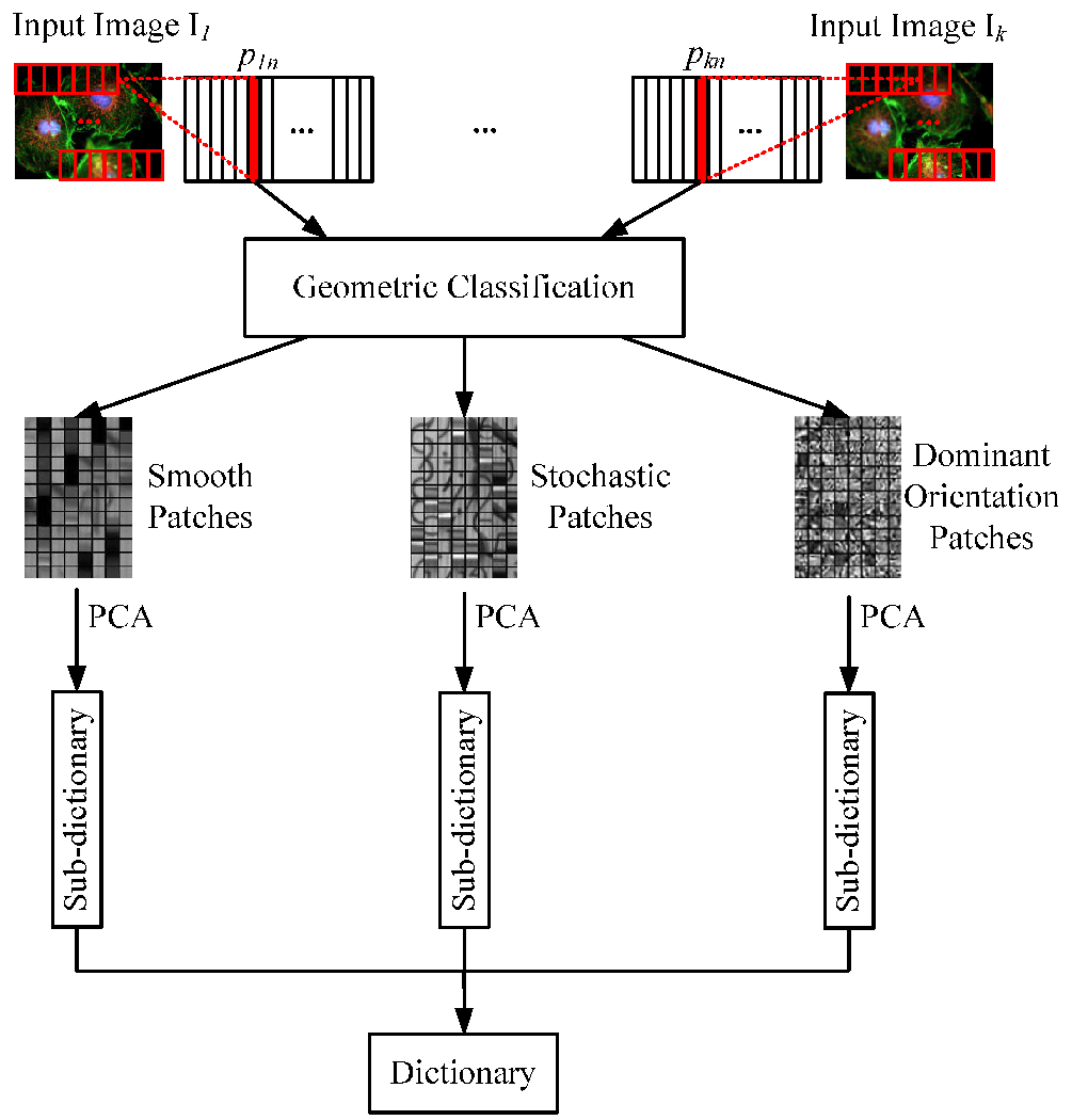
• In the first step, input source images are split into small blocks. According to the similarity of geometric patterns, these blocks are classified into smooth patches, stochastic patches, and dominant orientation patches.
• In the second step, it does principal component analysis (PCA) on each type of patches to extract crucial bases. The extracted PCA bases are used to construct the sub-dictionary of each image patch group.
• In the last step, the obtained sub-dictionaries are merged into a complete dictionary for sparse-representation-based fusion approach and the integrated sparse coefficients are inverted to fused image.

This paper has two main contributions.

• A geometric image patches classification method is proposed for dictionary learning. The proposed geometry classification method can accurately split source image patches into different image patch groups for dictionary learning. Dictionary bases extracted from each image patch group have good performance, when they are used to describe the geometric features of source images.
• A PCA-based geometry dictionary construction method is proposed. The trained dictionary with PCA bases is informative and compact for sparse representation. The informative feature of trained dictionary ensures that different geometric features of source images can be accurately described. The compact feature of trained dictionary can speed up the sparse coding process.

The rest sections of this paper are structured as follows: Section 2 proposes the geometric dictionary learning method and multi-focus image fusion framework; Section 3 compares and analyzes experimentation results; and Section 4 concludes this paper.

2. Geometry Dictionary Construction and Fusion Scheme

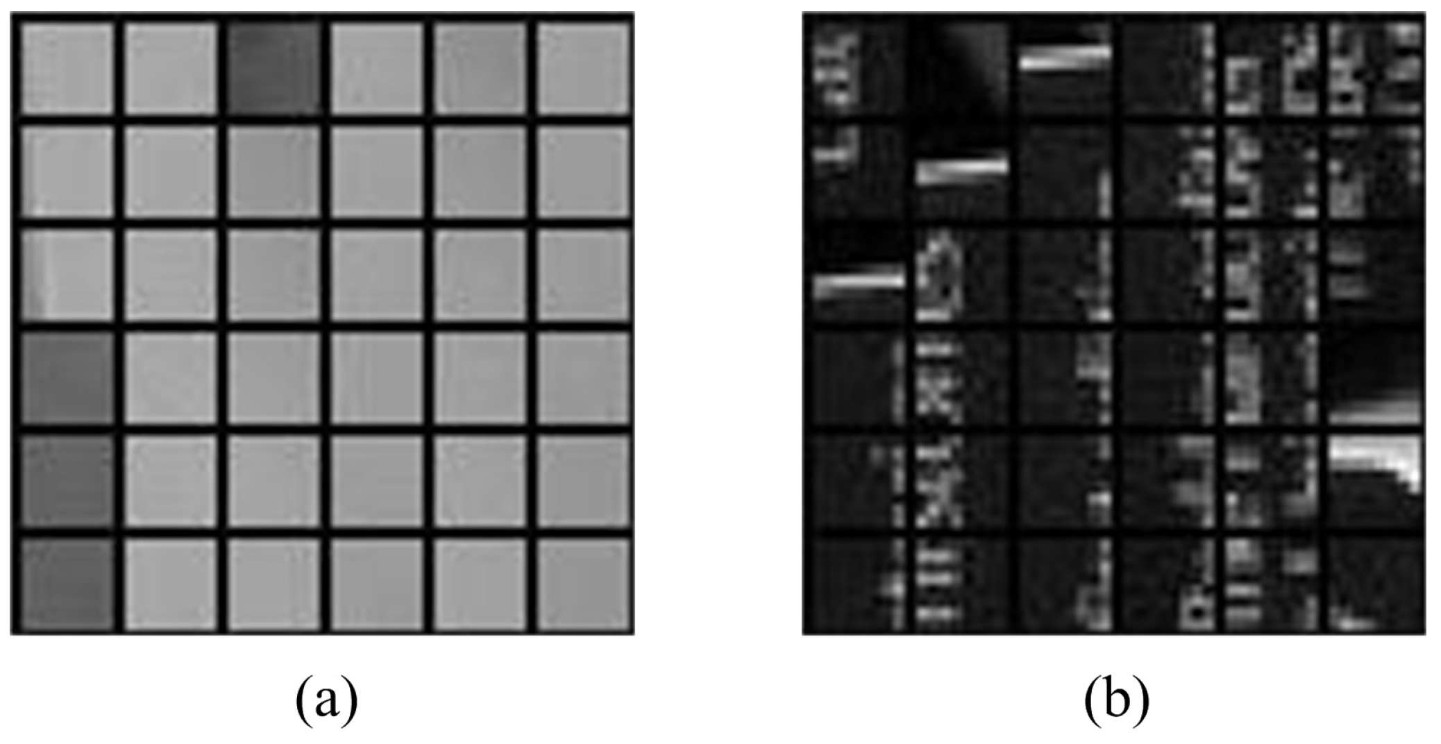
2.1. Dictionary Learning Analysis

During the sparse representation of the dictionary construction process, the key step is to construct an over-complete dictionary that covers the important information of input image. Since geometry information of image plays an important role in describing an image, an informative dictionary should take the geometric information into consideration. Smooth and non-smooth information as two important types of geometry information can be used to classify source images.

A multiple geometry information classification approach was proposed for single image super-resolution reconstruction (SISR) [39]. According to the geometric features, a large number of high-resolution (HR) image patches were randomly extracted and clustered to generate corresponding geometric dictionaries for sparse representations of local patches in low-resolution (LR) images. The geometric features were classified into three types, smooth patch, dominant orientation patch, and stochastic patch. According to the estimated dominant orientation, the dominant orientation patches could be divided into different directional patches. Rather than adaptively selecting one dictionary, the recovered patches were weighted in the learned geometric dictionaries to characterize the local image patterns, by a subsequent patch aggregation to estimate the whole image. To reduce the redundancy in image recovery, the self-similarity constraints were added on HR image patch aggregation. Both LR and HR residual images were estimated from the recovered image and compensated for the subtle details of reconstructed image.

In SISR, the source images are classified as smooth, dominant orientation, and stochastic patches. Dominant orientation and stochastic patches are non-smooth patches. Since the detection of orientation in finite dimensional Euclidean spaces corresponded to fitting an axis or a plane by Fourier transformation of an n-dimensional structure, Bigün verified dominant orientation and stochastic patches can be separated by orientation estimation in the spatial domain based on the error of the fit [42].

In dictionary learning, the redundancy of trained dictionary is usually not considered. A redundant dictionary not only has high computational complexity, but cannot also obtain the best effect in image representation. Different methods are proposed to reduce the redundancy in learning process to construct the compact dictionary. Elad [43] estimated the maximum a posteriori probability (MAP) by a compact dictionary. An effective image interpolation method by nonlocal autoregressive modeling (NARM) was developed and embedded in SRM by Dong [44] to enhance the effectiveness of SRM in image interpolation by reducing the coherence between the sampling matrix and the sparse representation dictionary and minimizing the nonlocal redundancy. To improve the performance of sparse representation-based image restoration, a non-locally centralized sparse representation (NCSR) model proposed by Dong [45] suppressed the sparse coding noise in image restoration.

The sparse representation-based approach linearly combines a few atoms extracted from an over-complete dictionary as an image patch. The promising results have been shown in various image restoration applications [38,45]. Based on the classification of image patches, this paper proposed sparse representation-based approach that uses PCA algorithm to construct more informative and compact dictionary [38]. The proposed solution cannot be extended to other sparse-representation applications. Most sparse representation methods are based on a large number of sample images. The corresponding learned dictionaries are expected to be applied to different scenic source images. The proposed solution uses sparse feature to do image sparse representation and fusion. Therefore, the learned dictionary of proposed solution does not need to be extended to different source images, and only specializes for experimented source images. It uses PCA classification to reduce the redundancy in dictionary and enhance the performance.

There are many popular dictionary learning methods like KSVD. However, this paper cannot use other dictionary learning methods to substitute PCA to do dictionary learning. It compares PCA with KSVD to explain the benefits of using PCA in dictionary learning. For sparse representation-based image reconstruction and fusion techniques, it is difficult to select a good over-complete dictionary. To obtain an adaptive dictionary, Aharon [46] developed KSVD that learned an over-complete dictionary by using a set of training images or updates a dictionary adaptively by applying SVD operations. The image patches used by KSVD in dictionary learning were extracted either from globally trained dictionary (natural images) or adaptively trained dictionary (input images). Although KSVD shows better performance in dictionary learning than other methods, it takes high costs to do dictionary learning with a large number of training images iteratively. The high computational complexity constrains the learned dictionary size of KSVD in practical usage. Kim [38] firstly applied clustering-based dictionary learning solution to image fusion. It clustered patches from different source images together based on local structural similarities. Only a few principal components of each cluster were analyzed and used to construct corresponding sub-dictionary. All learned sub-dictionaries were combined to form a compact and informative dictionary that can describe local structures of all source images effectively. The redundancies of dictionary (i.e., reducing the size of dictionary) were eliminated to reduce the computation loads of the proposed PCA-based dictionary learning solution. In various comparison experimentations, the proposed PCA-based dictionary learning solution (JPDL) had better performance than other traditional multi-scale transform-based and sparse representation-based methods, including KSVD. Comparing with KSVD, JPDL as a PCA-based method not only obtained a more compact dictionary, but also took less computational costs in dictionary learning process.

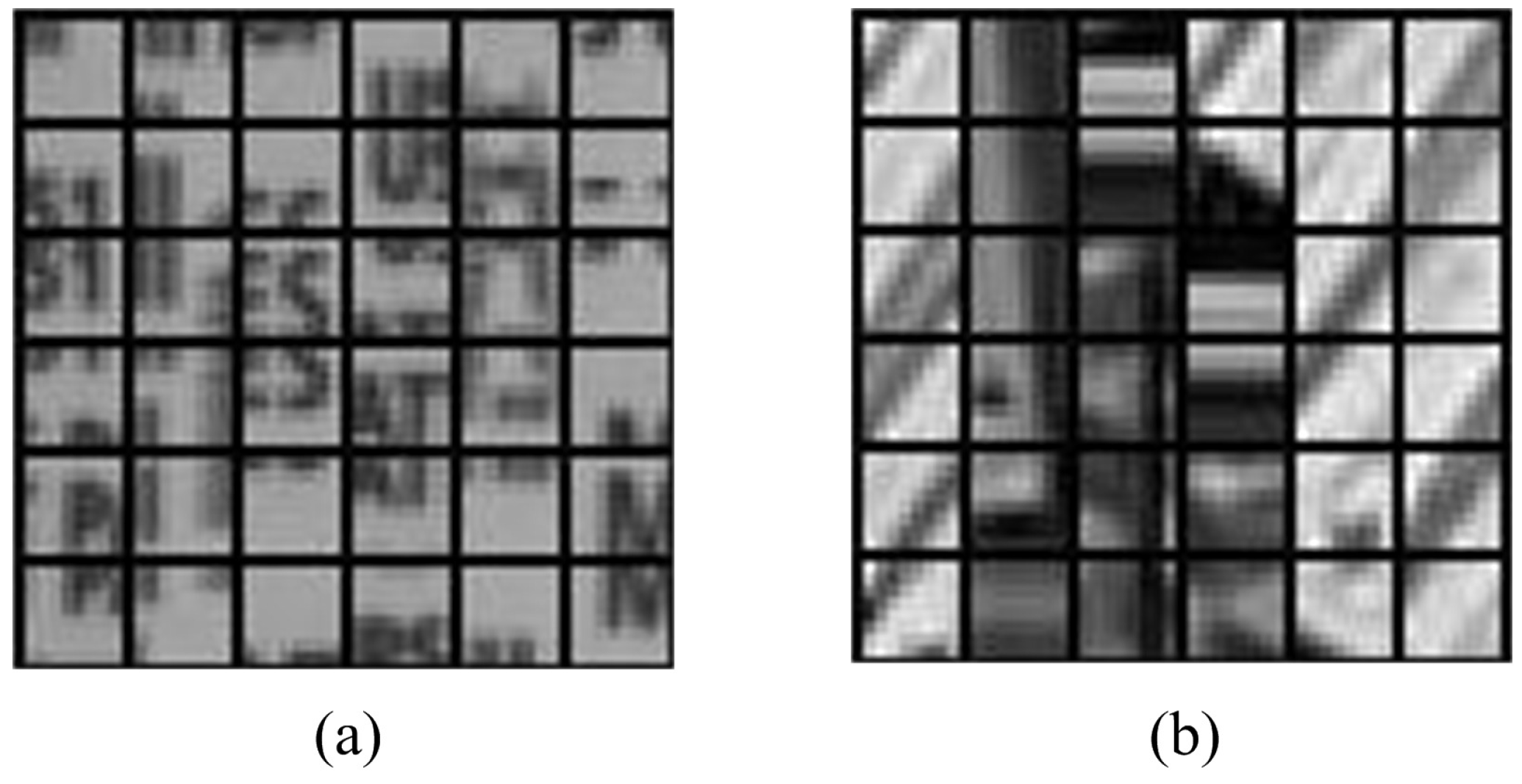
2.2. Geometry Dictionary Construction

According to geometric patterns used in SISR [39], this paper classifies the image into three patch types: smooth patches, stochastic patches, and dominant orientation patches. The smooth patches, stochastic patches and dominant orientation patches mainly describe the structure information, texture information, and edge information respectively. Based on a priori knowledge, image patches can be classified into three groups for sub-dictionaries learning. Additionally, to obtain more compact sub-dictionary for each image patch group, this paper uses PCA method to extract the important information from each group. PCA bases of each group are used as the bases of corresponding sub-dictionary. The obtained dictionary can be more compact and informative by combining the PCA-based sub-dictionaries [38].

This paper learns three different sub-dictionaries rather other one dictionary. Three different sub-dictionaries contain more detailed information and structure information, and less redundant information. It means that although the obtained sub-dictionaries are compact, they can still contain more useful information. Three types of geometric patches extract different image information from source images respectively.

• Smooth patches describe the structure information of source images, such as the background.
• Dominant orientation patches describe the edge information to provide the direction information in source images.
• Stochastic patches show the texture information to make up the missing detailed information that is not represented in dominant orientation patches.

Three learned dictionaries specialize in smooth, dominant orientation, and stochastic patches respectively. The structure information, edge information, and texture information can be accurately and completely shown in corresponding sub-dictionary. Comparing with one learned dictionary, three learned sub-dictionaries can not only supply different information of source images respectively, but also make up the deficiencies mutually to enhance the quality of merged dictionary. So each sub-dictionary is important to compose a compact and informative dictionary in the proposed approach.

The proposed geometric approach is shown in Figure 1 that has two main steps. In the first step, the input source images $I_i$ to $I_k$ are split to several small image blocks $p_{in},i\in (1,2...k),n\in (1,2...w)$, where i is the source image number, and n is the patch number. The total block number of each input image is w. Then according to the similarity of geometric patterns, the obtained image blocks are classified into three groups, smooth patch group, stochastic patch group, and dominant orientation patch group. In the second step, it does PCA analysis on each sub-class for extracting corresponding PCA bases as sub-dictionary. Then these obtained sub-dictionaries are composed to construct a complete dictionary for image sparse representation.

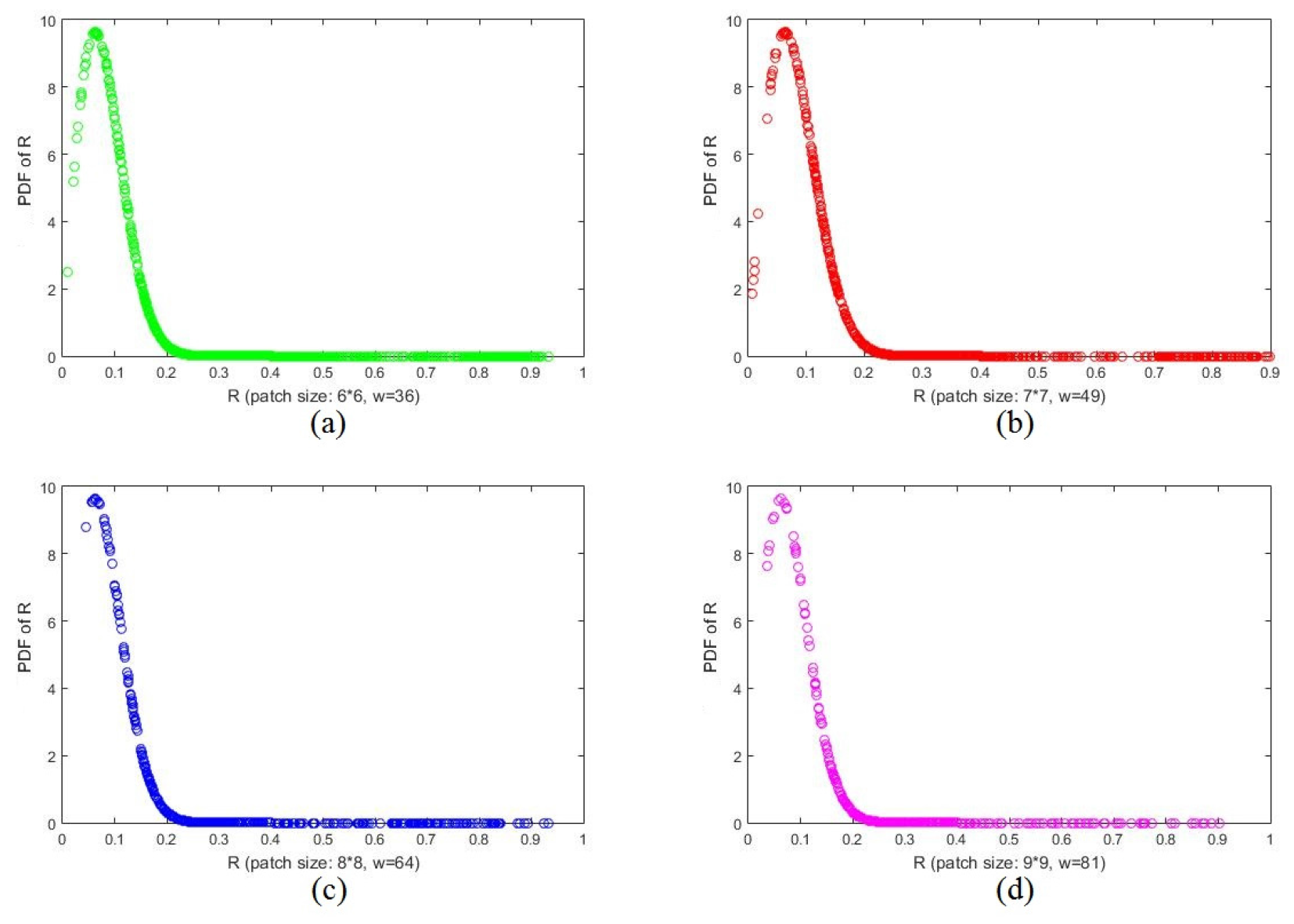
2.3. Geometric-Structure-Based Patches Classification

Image blocks of a source image can be classified by various image features in describing underlying relationships. According to geometry descriptions, the multi-focus source images can be divided to smooth, stochastic, and dominant orientation patches. The edges of focused area are usually sharp that contain dominant orientation patches. The out-of-focused areas are smooth that contain a large number of smooth blocks. Besides that, there are also lots of stochastic blocks in source images. Grouping image blocks into different classes for dictionary learning is an efficient way to improve the accuracy of image description.

To obtain different geometry sub-classes, this paper uses a geometric-structure-based approach to partition image into several sub-classes first. Then based on the classified image blocks, it gets the corresponding sub-dictionaries.

Before doing geometry analysis, it needs to divide the input image into $\sqrt{w}\times \sqrt{w}$ small image blocks $P_I=(p_1,p_2,...,p_n)$ first. Each image patch $p_i,i\in (1,2,...n)$ is converted into $1\times w$ image vectors $v_i,i\in (1,2,...n)$. After obtaining vectors , the variance $C_i$ of pixels in each image vector can be calculated. After obtaining variance, it needs to choose the threshold δ to evaluate whether image block is smooth. If $C_i<\delta$, image block $p_i$ is smooth, otherwise image block $p_i$ is not smooth [39]. Based on the threshold δ, the classified smooth and non-smooth patches are shown in Figure 2a,b respectively.

According to the classified smooth and non-smooth patches shown in Figure 2a,b, it is clear to find that the smooth patches have similar structure information of input images. Oppositely, non-smooth patches are different and cannot be directly classified into one class.

Non-smooth patches may also be classified. According to geometric patterns, non-smooth patches could be divided into stochastic and dominant orientation patches. The separation method of stochastic and dominant orientation image patches consists of two steps. In the first step, the gradient of each pixel is calculated. In every image vector $v_i,i\in (1,2,...n)$, the gradient of each pixel $k_{ij}$, $j\in (1,2,...,w),i\in (1,2,...n)$ is composed by its x and y coordinate gradient $g_{ij}\left(x\right)$ and $g_{ij}\left(y\right)$. The gradient value of each pixel $k_{ij}$ in image patch $v_i$ is $g_{ij}=(g_{ij}\left(x\right),g_{ij}\left(y\right))$. The $(g_{ij}\left(x\right)$, $g_{ij}\left(y\right))$ can be calculated by $g_{ij}\left(x\right)=\partial k_{ij}(x,y)/\partial x$, $g_{ij}\left(y\right)=\partial k_{ij}(x,y)/\partial y$. For each image vector $v_i$, the gradient $G_i$ is $G_i={(g_{i1},g_{i2},...,g_{iw})}^T$, where $G_i\in {\mathbb{R}}^{w\times 2}$. In the second step, the gradient value of each image patch is decomposed by Equation (1):

$$\begin{array}{c}\hfill \begin{array}{c}\hfill G_i=\left[\begin{array}{c}{G}_{i1}\\ G_{i2}\\ ...\\ G_{iw}\end{array}\right]=U_i{S}_i{V}_i^T\end{array},\end{array}$$

(1)

where $U_i{S}_i{V}_i^T$ is the singular value decomposition of $G_i$. $S_i$ is a diagonal $2\times 2$ matrix for representing energy in dominant directions [47]. When $S_i$ is obtained, the dominant measure R can be calculated. The calculation method of R is shown in Equation (2):

$$\begin{array}{c}\hfill \begin{array}{c}\hfill R=\frac{S_{1,1}-S_{2,2}}{S_{1,1}+S_{2,2}}\end{array},\end{array}$$

(2)

The smaller the R is, the more stochastic the corresponding image patch is [48]. In this case, a threshold $R^{*}$ should be calculated for distinguishing stochastic and dominant orientation patches. To find the threshold $R^{*}$, a probability density function (PDF) of R is calculated. According to [42], the PDF of R can be calculated by Equation (3).

$$\begin{array}{c}\hfill \begin{array}{c}\hfill P\left(R\right)=4(w-1)R\frac{{(1-R^2)}^{w-2}}{{(1+R^2)}^w}\end{array},\end{array}$$

(3)

The PDF of dominant measure R of patches with different sizes is shown in Figure 3.

A PDF significance test is implemented to distinguish stochastic and dominant orientation patch by the threshold $R^{*}$ [42]. If R is less than $R^{*}$, the image patch can be considered as stochastic patch. The stochastic and dominant orientation patches separated by the proposed method are shown in Figure 4. The Figure 4a shows the stochastic image patches, which contain some texture and detailed information. Dominant orientation image patches are shown in Figure 4b, which mainly contain the edge information.

As shown in Figure 3, when R increases, $P\left(R\right)$ converges to zero. It chooses the value of R as the threshold $R^{*}$, when $P\left(R\right)$ reaches zero for the first time.

2.4. PCA-Based Dictionary Construction

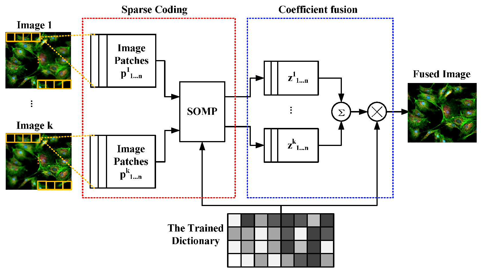
When the geometric classification finished, image patches with similar geometric structure are classified into a few groups. In this work, the compact and informative dictionary is trained by combining the principal components of each geometric group. Since patches in the same geometric group can be well-approximated by a small number of PCA bases, top m most informative principal components are chosen to form a sub-dictionary [49] as Equation (4).

$$\begin{array}{c}\hfill \begin{array}{c}\hfill B_x=[b_1,b_2...,b_j],s.t.p=\underset{p}{\arg \max }\left\{\sum _{j=p+1}^q{L}_j>\delta \right\}\end{array},\end{array}$$

(4)

where $B_x$ denotes the sub-dictionary of the xth cluster, and q is the total number of atoms in each cluster. Each $B_x$ consists of p eigenvector atoms. $L_j$ is the eigenvalue of the corresponding jth eigenvector $d_j$. The eigenvalues are sorted in descending order (i.e., $L_1>L_2>...>L_n>0$). δ is a parameter to control the amount of approximation with rank p. Usually, δ is set to a proportional to the dimension of input image to avoid over-fitting [49]. After the sub-dictionaries are obtained, a dictionary D is constructed by combining sub-dictionaries together as Equation (5).

$$\begin{array}{c}\hfill \begin{array}{c}\hfill D=[B_1,B_2...,B_n]\end{array},\end{array}$$

(5)

where n is the total number of clusters.

2.5. Fusion Scheme

The fusion scheme of proposed method is shown in Figure 5, which consists of two steps.

In the first step, each input image $I_i$ is split into n image patches with the size of $\sqrt{w}\times \sqrt{w}$. These image patches are resized to $w*1$ vectors $p_1^i,p_2^i,...,p_n^i$. The resized vectors are sparse coded with trained dictionary to sparse coefficients $z_1^i,z_2^i,...,z_n^i$. In the second step, the sparse coefficients are fused by ’Max-L1’ fusion rule [50,51,52]. Then the fused coefficients are inverted to fused image by the trained dictionary.

3. Experiments and Analyses

In comparison experiments, three pairs of color fluorescence images are used to test the proposed multi-focused image fusion approach. All three multi-focus image pairs are modified to the size of $256\times 256$ for comparison purpose. To show the efficiency of proposed method, the state of art dictionary learning based sparse-representation fusion schemes KSVD [50] and JPDL [38], which were proposed by Li in 2012 and Kim in 2016 respectively, are used in comparison experiments. The comparison experiments are evaluated by both subjective and objective assessments. Four popular image fusion quality metrics are used in this paper for the quantitative evaluation. The patch size of all sparse-representation-based methods including the proposed method are set to $8\times 8$. To avoid blocking artifacts, all experiments use sliding window scheme [38,50]. The overlapped region of sliding window scheme is set to 4-pixel in each vertical and horizontal direction of all experiments. All experiments were implemented using Matlab, version 2014a; MathWorks: Natick, MA, 2014, and Visual Studio, version Community 2013; Microsoft: Redmond, WA, 2013, mixed programming on an Intel(R) Core(TM), version i7-4720HQ; Intel: Santa Clara, CA, 2015, CPU @ 2.60 GHz Laptop with 12.00 GB RAM.

3.1. Objective Evaluation Methods

Five mainstream objective evaluation metrics are implemented for the quantitative evaluation. These metrics include edge retention ($Q^{AB/F}$) [53,54], mutual information (MI) [55], visual information fidelity (VIF) [56], Yang proposed fusion metric ($Q_Y$) [57,58], and Chen-Blum metric ($Q_{CB}$) [58,59]. For the fused image, the sizes of $Q^{AB/F}$, MI, VIF, $Q_Y$, and $Q_{CB}$ become bigger, the corresponding fusion results are better.

3.1.1. Mutual Information

MI for images can be formalized as Equation (6).

$$\begin{array}{c}\hfill \begin{array}{c}\hfill MI=\sum _{i=1}^L\sum _{j=1}^L{h}_{A,F}(i,j)lo{g}_2\frac{h_{A,F}(i,j)}{h_A\left(i\right)h_{F\left(j\right)}}\end{array},\end{array}$$

(6)

where L is the number of gray-level, $h_{R,F}(i,j)$ is the gray histogram of image A and F. $h_A\left(i\right)$ and $h_F\left(j\right)$ are edge histogram of image A and F. MI of fused image can be calculated by Equation (7).

$$\begin{array}{c}\hfill \begin{array}{c}\hfill MI(A,B,F)=MI(A,F)+MI(B,F)\end{array},\end{array}$$

(7)

where $MI(A,F)$ represents the MI value of input image A and fused image F; $MI(B,F)$ represents the MI value of input image B and fused image F.

3.1.2. $Q^{AB/F}$

$Q^{AB/F}$ metric is a gradient-based quality index to measure how well the edge information of source images conducted to the fused image. It is calculated by:

$$\begin{array}{c}\hfill \begin{array}{c}\hfill Q^{AB/F}=\frac{{\sum }_{i,j}(Q^{AF}(i,j)w^A(i,j)+Q^{BF}(i,j)w^B(i,j))}{{\sum }_{i,j}(w^A(i,j)+w^B(i,j))}\end{array},\end{array}$$

(8)

where $Q^{AF}=Q_g^{AF}{Q}_0^{AF}$, $Q_g^{AF}$ and $Q_0^{AF}$ are the edge strength and orientation preservation values at location (i, j). $Q^{BF}$ can be computed similarly to $Q^{AF}$ . $w_A(i,j)$ and $w_B(i,j)$ are the weights of $Q^{AF}$ and $Q^{BF}$ respectively.

3.1.3. Visual Information Fidelity

VIF is the novel full reference image quality metric. VIF quantifies the mutual information between the reference and test images based on Natural Scene Statistics (NSS) theory and Human Visual System (HVS) model. It can be expressed as the ratio between the distorted test image information and the reference image information, the calculation equation of VIF is shown in Equation (9).

$$\begin{array}{c}\hfill \begin{array}{c}\hfill VIF=\frac{{\sum }_{i\in subbands}I(\overrightarrow{C^{N,i}};\overrightarrow{F^{N,i}})}{{\sum }_{i\in subbands}I(\overrightarrow{C^{N,i}};\overrightarrow{E^{N,i}})}\end{array},\end{array}$$

(9)

where $I(\overrightarrow{C^{N,i}};\overrightarrow{F^{N,i}})$ and $I(\overrightarrow{C^{N,i}};\overrightarrow{E^{N,i}})$ represent the mutual information, which are extracted from a particular subband in the reference and the test images respectively. $\overrightarrow{C^N}$ denotes N elements from a random field, $\overrightarrow{E^N}$ and $\overrightarrow{F^N}$ are visual signals at the output of HVS model from the reference and the test images respectively.

To evaluate the VIF of fused image, an average of VIF values of each input image and the integrated image is proposed [56]. The evaluation function of VIF for image fusion is shown in Equation (10).

$$\begin{array}{c}\hfill \begin{array}{c}\hfill VIF(A,B,F)=\frac{VIF(A,F)+VIF(B,F)}{2}\end{array},\end{array}$$

(10)

where $VIF(A,F)$ is the VIF value between input image A and fused image F; $VIF(B,F)$ is the VIF value between input image B and fused image F.

3.1.4. $Q_Y$

Yang et al. proposed structural similarity-Based way for fusion assessment [57]. The Yang’s method is shown in Equation (11).

$$\begin{array}{c}\hfill \begin{array}{c}\hfill Q_Y=\left\{\begin{array}{c}\begin{array}{c}\lambda \left(\omega \right)SSIM(A,F\left|\omega \right.)+(1-\lambda \left(\omega \right)(SSIM(B,F\left|\omega \right.),\hfill \\ SSIM(A,B\left|\omega \right.)\ge 0.75,\hfill \end{array}\\ \begin{array}{c}max\left\{SSIM(A,F\left|\omega \right.),SSIM(A,B\left|\omega \right.)\right\},\hfill \\ SSIM(A,B\left|\omega \right.)<0.75\hfill \end{array}\end{array}\right.\end{array},\end{array}$$

(11)

where $\lambda \left(\omega \right)$ is the local weight, $SSIM(A,B)$ is a structural similarity index measure for images A and B. The detail of $\lambda \left(\omega \right)$ and $SSIM(A,B)$ can be found in [57,58].

3.1.5. $Q_{CB}$

Chen-Blum metric is human perception inspired fusion metrics. Chen-Blum metric consists of 5 steps:

In the first step, filtering image $I(i,j)$ in frequency domain. $I(i,j)$ is transformed to frequency domain and get $I(m,n)$. Filtering $I(m,n)$ by contrast sensitive function(CSV) [59] filter $S\left(r\right)$, where $r=\sqrt{m^2+n^2}$. In this image fusion metric $S\left(r\right)$ is in polar form. $\tilde{I}(m,n)$ can be got by $\tilde{I}(m,n)=I(m,n)*S\left(r\right)$.

In the second step, local contrast is computed. For $Q_{CB}$ metric, Peli’s contrast is used and it can be defined as:

$$\begin{array}{c}\hfill \begin{array}{c}\hfill C(i,j)=\frac{{\varphi }_k(i,j)*I(i,j)}{{\varphi }_{k+1}(i,j)*I(i,j)}-1\end{array}.\end{array}$$

(12)

A common choice for ${\varphi }_k(i,j)$ would be

$$\begin{array}{c}\hfill \begin{array}{c}\hfill {\varphi }_k(i,j)=\frac{1}{\sqrt{2\pi }{\sigma }_k}{e}^{\frac{i^2+j^2}{2{\sigma }_k^2}}\end{array}.\end{array}$$

(13)

with a standard deviation ${\sigma }_k=2$.

In the third step, The masked contrast map for input image $I_A(i,j)$ is calculated as:

$$\begin{array}{c}\hfill \begin{array}{c}\hfill C_A^{\prime }=\frac{t{\left(C_A\right)}^p}{h{\left(C_A\right)}^p+Z}\end{array}.\end{array}$$

(14)

Here, $t,h,p,q$ and Z are real scalar parameters that determine the shape of the nonlinearity of the masking function [59,60].

In the fourth step, the saliency map of $I_A(i,j)$ can be calculated by Equation (15),

$$\begin{array}{c}\hfill \begin{array}{c}\hfill {\lambda }_A(i,j)=\frac{{C_A^{\prime }}^2(i,j)}{{C_A^{\prime }}^2(i,j)+{C_A^{\prime }}^2(i,j)}\end{array}.\end{array}$$

(15)

The information preservation value is computed as Equation (16),

$$\begin{array}{c}\hfill \begin{array}{c}\hfill Q_{AF}(i,j)=\left\{\begin{array}{c}\frac{C_A^{\prime }(i,j)}{C_F^{\prime }(i,j)},if{C}_A^{\prime }(i,j)<C_F^{\prime }(i,j),\\ \frac{C_F^{\prime }(i,j)}{C_A^{\prime }(i,j)},otherwise.\end{array}\right.\end{array}\end{array}$$

(16)

In the fifth step, the Global quality map can be calculated:

$$\begin{array}{c}\hfill \begin{array}{c}\hfill Q_{GQM}(i,j)={\lambda }_A(i,j)Q_{AF}(i,j)+{\lambda }_B(i,j)Q_{BF}(i,j)\end{array}.\end{array}$$

(17)

Then the value of $Q_{CB}$ can be got by average the global quality map:

$$\begin{array}{c}\hfill \begin{array}{c}\hfill Q_{CB}=\overline{\sum _{i,j}{Q}_{GQM}(i,j)}\end{array}.\end{array}$$

(18)

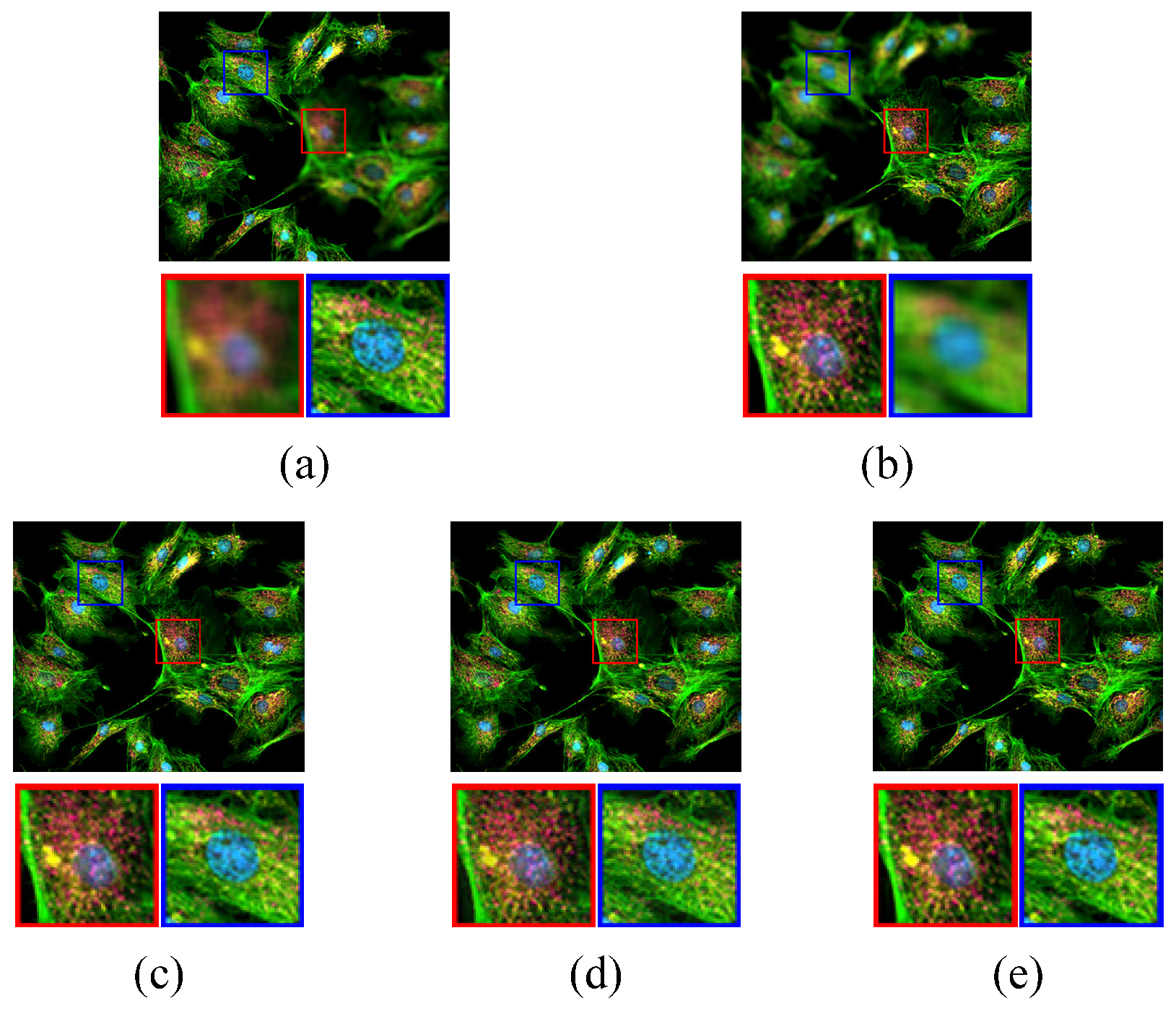
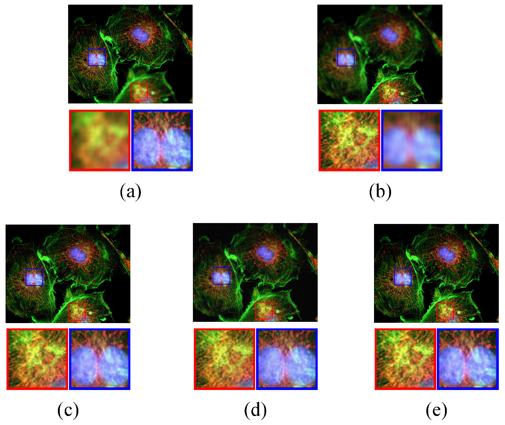
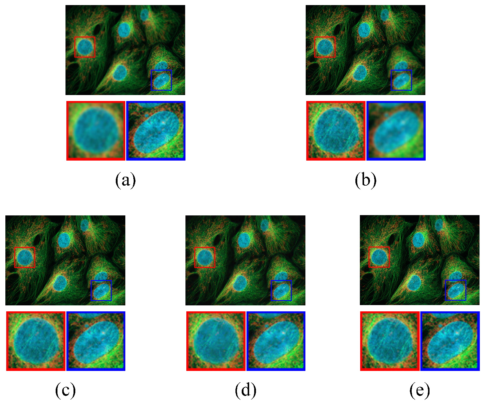
3.2. Image Quality Comparison

To show the efficiency of proposed method, the quality comparison of fused images is demonstrated. It compares the quality of fused image based on visual effect, the accuracy of focused region detection, and the objective evaluations.

3.2.1. Comparison Experiment 1

The source fluorescence image is obtained from public website [61]. Figure 6a,b are the source multi-focus fluorescence images. To show the details of fused image, two image blocks are highlighted and magnified, which are squared by red and blue square respectively. The image block in red square is out of focus in Figure 6a, and the image block in blue square, is out of focus in Figure 6b. The corresponding image block in blue and red square are totally focused in Figure 6a,b respectively. Figure 6c–e show the fused images of KSVD, JPDL, and proposed method, respectively.

The difference and performance of fused images by three different methods are difficult to figure out by eyes. In order to evaluate of fusion performances objectively, $Q^{AB/F}$, MI, VIF, $Q_Y$, and $Q_{CB}$ are also used as image fusion quality measures. The fusion results of multi-focus fluorescence images using three different methods are shown in

Table 1. Fusion Performance Comparison - 1 of Multi-focus Fluorescence Image Pairs.

	${\mathit{Q}}^{\mathit{AB}/\mathit{F}}$	MI	VIF	${\mathit{Q}}_{\mathit{Y}}$	${\mathit{Q}}_{\mathit{CB}}$
KSVD	0.4966	2.4247	0.5778	0.5960	0.5287
JPDL	0.5815	2.9258	0.6972	0.6944	0.7243
Proposed Solution	0.6226${}^{*}$	3.4773	0.7428	0.7386	0.7974

* The highest result in each column is marked in bold-face.

.

The best results of each evaluation metric are highlighted by bold-faces in Table 1. According to Table 1, it can figure out that the proposed method has the best performance in all five types of evaluation metrics. Particularly, for the objective evaluation metric $Q^{AB/F}$, the proposed method obtains higher result than other two comparison image fusion methods. Since $Q^{AB/F}$ is a gradient-based quality metric to measure how well the edge information of source images is conducted to the fused image, it means the proposed method can get better fused image with edge information.

3.2.2. Comparison Experiment 2 and 3

Similarly, the source fluorescence images shown in Figure 7 and Figure 8a,b are obtained from public websites [62,63] respectively. In a set of source images, two images (a) and (b) focus on different items. The source images are fused by KSVD, JPDL, and proposed method to get a totally focused image, and the corresponding fusion results are shown in Figure 7 and Figure 8c–e respectively.

Objective metrics of multi-focus comparison experiment 2 and 3 are shown in

Table 2. Fusion Performance Comparison - 2 of Multi-focus Fluorescence Image Pairs.

	${\mathit{Q}}^{\mathit{AB}/\mathit{F}}$	MI	VIF	${\mathit{Q}}_{\mathit{Y}}$	${\mathit{Q}}_{\mathit{CB}}$
KSVD	0.5600	2.4747	0.6099	0.6161	0.5477
JPDL	0.6952	3.1357	0.7013	0.7355	0.7423
Proposed Solution	0.7692${}^{*}$	3.8982	0.7488	0.8058	0.8206

* The highest result in each column is marked in bold-face.

and

Table 3. Fusion Performance Comparison - 3 of Multi-focus Fluorescence Image Pairs.

	${\mathit{Q}}^{\mathit{AB}/\mathit{F}}$	MI	VIF	${\mathit{Q}}_{\mathit{Y}}$	${\mathit{Q}}_{\mathit{CB}}$
KSVD	0.6837	2.4624	0.8171	0.7855	0.6454
JPDL	0.8557	2.9358	0.8943	0.9325	0.7665
Proposed Solution	0.8979${}^{*}$	3.9154	0.9129	0.9790	0.8237

* The highest result in each column is marked in bold-face.

respectively to evaluate the quality of fused images. According to the metric results, the proposed method has the best performance in all five objective evaluations in comparison experiment 2 and 3. So the proposed method has the best overall performance among all comparison methods.

3.3. Processing Time Comparison

Table 4. Processing Time Comparison.

	Experiment - 1	Experiment - 2	Experiment - 3
KSVD	164.02 s	215.09 s	108.65 s
JPDL	123.68 s	171.93 s	73.58 s
Proposed Solution	76.23 s${}^{*}$	103.96 s	25.47 s

* The highest result in each column is marked in bold-face.

compares the processing times of three comparison experimentations. The proposed solution has lower computation costs than KSVD and JPDL in image fusion process. Compared with KSVD, the dictionary construction method of proposed solution does not use any iterative way to extract the underlying information of images, which is not efficient in dictionary construction. Although JPDL and the proposed method both cluster image pixels or patches based on geometric similarity, the proposed method does not use the iterative method of Steering Kernel Regression (SKR), which is time consuming.

4. Conclusions

This paper proposes a novel sparse representation-based image fusion framework, which integrates geometric dictionary construction. A geometric image patch classification approach is presented to group image patches from different source images based on the similarity of image geometric structure. The proposed method extracts a few compact and informative sub-dictionaries from each image patch cluster by PCA and these sub-dictionaries are combined into a dictionary for sparse representation. Then image patches are sparsely coded into coefficients by the trained dictionary. For obtaining better edge and corner details of fusion results, the proposed solution also chooses image block size adaptively and selects optimal coefficients during the image process. The sparsely coded coefficients are fused by Max-L1 rule and inverted to the fused image. The proposed method is compared with existing mainstream sparse representation-based methods in various experiments. The experimentation results proves that the proposed method has good fusion performance in different image scenarios.

References

1. Tsai, W.; Qi, G. DICB: Dynamic Intelligent Customizable Benign Pricing Strategy for Cloud Computing. In Proceedings of the 5th IEEE International Conference on Cloud Computing, Honolulu, HI, USA, 24–29 June 2012; pp. 654–661.
2. Wu, W.; Tsai, W.; Jin, C.; Qi, G.; Luo, J. Test-Algebra Execution in a Cloud Environment. In Proceedings of the 8th IEEE International Symposium on Service Oriented System Engineering, SOSE 2014, Oxford, UK, 7–11 April 2014; pp. 59–69.
3. Tsai, W.; Qi, G.; Chen, Y. Choosing cost-effective configuration in cloud storage. In Proceedings of the 11th IEEE International Symposium on Autonomous Decentralized Systems, ISADS 2013, Mexico City, Mexico, 6–8 March 2013; pp. 1–8.
4. Li, X.; Li, H.; Yu, Z.; Kong, Y. Multifocus image fusion scheme based on the multiscale curvature in nonsubsampled contourlet transform domain. Opt. Eng. 2015, 54, 073115-1–073115-15. [Google Scholar] [CrossRef]
5. Rodger, J.A. Toward reducing failure risk in an integrated vehicle health maintenance system: A fuzzy multi-sensor data fusion Kalman filter approach for {IVHMS}. Expert Syst. Appl. 2012, 39, 9821–9836. [Google Scholar] [CrossRef]
6. Li, H.; Li, X.; Yu, Z.; Mao, C. Multifocus image fusion by combining with mixed-order structure tensors and multiscale neighborhood. Inf. Sci. 2016, 349–350, 25–49. [Google Scholar] [CrossRef]
7. Sun, J.; Zheng, H.; Chai, Y.; Hu, Y.; Zhang, K.; Zhu, Z. A direct method for power system corrective control to relieve current violation in transient with UPFCs by barrier functions. Int. J. Electr. Power & Energy Syst. 2016, 78, 626–636. [Google Scholar]
8. Li, S.; Kang, X.; Hu, J.; Yang, B. Image matting for fusion of multi-focus images in dynamic scenes. Inf. Fusion 2013, 14, 147–162. [Google Scholar] [CrossRef]
9. Li, H.; Liu, X.; Yu, Z.; Zhang, Y. Performance improvement scheme of multifocus image fusion derived by difference images. Signal Process. 2016, 128, 474–493. [Google Scholar] [CrossRef]
10. Nejati, M.; Samavi, S.; Shirani, S. Multi-focus image fusion using dictionary-based sparse representation. Inf. Fusion 2015, 25, 72–84. [Google Scholar] [CrossRef]
11. Li, S.; Yang, B. Multifocus image fusion using region segmentation and spatial frequency. Image Vis. Comput. 2008, 26, 971–979. [Google Scholar] [CrossRef]
12. Li, H.; Yu, Z.; Mao, C. Fractional differential and variational method for image fusion and super-resolution. Neurocomputing 2016, 171, 138–148. [Google Scholar] [CrossRef]
13. Li, H.; Qiu, H.; Yu, Z.; Zhang, Y. Infrared and visible image fusion scheme based on NSCT and low-level visual features. Infrared Phys. Technol. 2016, 76, 174–184. [Google Scholar] [CrossRef]
14. Li, S.; Yang, B.; Hu, J. Performance comparison of different multi-resolution transforms for image fusion. Inf. Fusion 2011, 12, 74–84. [Google Scholar] [CrossRef]
15. Vijayarajan, R.; Muttan, S. Discrete wavelet transform based principal component averaging fusion for medical images. Int. J. Electron. Commun. 2015, 69, 896–902. [Google Scholar] [CrossRef]
16. Pajares, G.; de la Cruz, J.M. A wavelet-based image fusion tutorial. Pattern Recognit. 2004, 37, 1855–1872. [Google Scholar] [CrossRef]
17. Makbol, N.M.; Khoo, B.E. Robust blind image watermarking scheme based on Redundant Discrete Wavelet Transform and Singular Value Decomposition. Int. J. Electron. Commun. 2013, 67, 102–112. [Google Scholar] [CrossRef]
18. Luo, X.; Zhang, Z.; Wu, X. A novel algorithm of remote sensing image fusion based on shift-invariant Shearlet transform and regional selection. Int. J. Electron. Commun. 2016, 70, 186–197. [Google Scholar] [CrossRef]
19. Liu, X.; Zhou, Y.; Wang, J. Image fusion based on shearlet transform and regional features. Int. J. Electron. Commun. 2014, 68, 471–477. [Google Scholar] [CrossRef]
20. Sulochana, S.; Vidhya, R.; Manonmani, R. Optical image fusion using support value transform (SVT) and curvelets. Optik-Int. J. Light Electron Opt. 2015, 126, 1672–1675. [Google Scholar] [CrossRef]
21. Zhu, Z.; Chai, Y.; Yin, H.; Li, Y.; Liu, Z. A novel dictionary learning approach for multi-modality medical image fusion. Neurocomputing 2016, 214, 471–482. [Google Scholar] [CrossRef]
22. Seal, A.; Bhattacharjee, D.; Nasipuri, M. Human face recognition using random forest based fusion of à-trous wavelet transform coefficients from thermal and visible images. Int. J. Electron. Commun. 2016, 70, 1041–1049. [Google Scholar] [CrossRef]
23. Qu, X.B.; Yan, J.W.; Xiao, H.Z.; Zhu, Z.Q. Image Fusion Algorithm Based on Spatial Frequency-Motivated Pulse Coupled Neural Networks in Nonsubsampled Contourlet Transform Domain. Acta Autom. Sin. 2008, 34, 1508–1514. [Google Scholar] [CrossRef]
24. Tsai, W.; Qi, G. A Cloud-Based Platform for Crowdsourcing and Self-Organizing Learning. In Proceedings of the 8th IEEE International Symposium on Service Oriented System Engineering, SOSE 2014, Oxford, UK, 7–11 April 2014; pp. 454–458.
25. Elad, M.; Aharon, M. Image Denoising Via Learned Dictionaries and Sparse representation. In Proceedings of the 2006 IEEE Computer Society Conference on Computer Vision and Pattern Recognition (CVPR 2006), New York, NY, USA, 17–22 June 2006; pp. 895–900.
26. Tsai, W.T.; Qi, G. Integrated fault detection and test algebra for combinatorial testing in TaaS (Testing-as-a-Service). Simul. Model. Pract. Theory 2016, 68, 108–124. [Google Scholar] [CrossRef]
27. Zhu, Z.; Qi, G.; Chai, Y.; Yin, H.; Sun, J. A Novel Visible-infrared Image Fusion Framework for Smart City. Int. J. Simul. Process Model. 2016, in press. [Google Scholar]
28. Han, J.; Yue, J.; Zhang, Y.; Bai, L. Local Sparse Structure Denoising for Low-Light-Level Image. IEEE Trans. Image Process. 2015, 24, 5177–5192. [Google Scholar] [CrossRef] [PubMed]
29. Zhang, X.; Zhang, S. Diffusion scheme using mean filter and wavelet coefficient magnitude for image denoising. Int. J. Electron. Commun. 2016, 70, 944–952. [Google Scholar] [CrossRef]
30. Sun, J.; Chai, Y.; Su, C.; Zhu, Z.; Luo, X. BLDC motor speed control system fault diagnosis based on LRGF neural network and adaptive lifting scheme. Appl. Soft Comput. 2014, 14, 609–622. [Google Scholar] [CrossRef]
31. Xu, J.; Feng, A.; Hao, Y.; Zhang, X.; Han, Y. Image deblurring and denoising by an improved variational model. Int. J. Electron. Commun. 2016, 70, 1128–1133. [Google Scholar] [CrossRef]
32. Shi, J.; Qi, C. Sparse modeling based image inpainting with local similarity constraint. In Proceedings of the IEEE International Conference on Image Processing, ICIP 2013, Melbourne, Australia, 15–18 September 2013; pp. 1371–1375.
33. Aslantas, V.; Bendes, E. A new image quality metric for image fusion: The sum of the correlations of differences. Int. J. Electron. Commun. 2015, 69, 1890–1896. [Google Scholar] [CrossRef]
34. Yang, J.; Wright, J.; Huang, T.S.; Ma, Y. Image Super-Resolution Via Sparse Representation. IEEE Trans. Image Process. 2010, 19, 2861–2873. [Google Scholar] [CrossRef] [PubMed]
35. Yang, B.; Li, S. Multifocus Image Fusion and Restoration With Sparse Representation. IEEE Trans. Instrum. Meas. 2010, 59, 884–892. [Google Scholar] [CrossRef]
36. Li, H.; Li, L.; Zhang, J. Multi-focus image fusion based on sparse feature matrix decomposition and morphological filtering. Opt. Commun. 2015, 342, 1–11. [Google Scholar] [CrossRef]
37. Wang, J.; Liu, H.; He, N. Exposure fusion based on sparse representation using approximate K-SVD. Neurocomputing 2014, 135, 145–154. [Google Scholar] [CrossRef]
38. Kim, M.; Han, D.K.; Ko, H. Joint patch clustering-based dictionary learning for multimodal image fusion. Inf. Fusion 2016, 27, 198–214. [Google Scholar] [CrossRef]
39. Yang, S.; Wang, M.; Chen, Y.; Sun, Y. Single-Image Super-Resolution Reconstruction via Learned Geometric Dictionaries and Clustered Sparse Coding. IEEE Trans. Image Process. 2012, 21, 4016–4028. [Google Scholar] [CrossRef] [PubMed]
40. Sun, J.; Zheng, H.; Demarco, C.; Chai, Y. Energy Function Based Model Predictive Control with UPFCs for Relieving Power System Dynamic Current Violation. IEEE Trans. Smart Grid 2016, 7, 2933–2942. [Google Scholar] [CrossRef]
41. Keerqinhu; Qi, G.; Tsai, W.; Hong, Y.; Wang, W.; Hou, G.; Zhu, Z. Fault-Diagnosis for Reciprocating Compressors Using Big Data. In Proceedings of the Second IEEE International Conference on Big Data Computing Service and Applications, BigDataService 2016, Oxford, UK, 29 March–1 April 2016; pp. 72–81.
42. Bigün, J.; Granlund, G.H.; Wiklund, J. Multidimensional Orientation Estimation with Applications to Texture Analysis and Optical Flow. IEEE Trans. Pattern Anal. Mach. Intell. 1991, 13, 775–790. [Google Scholar] [CrossRef]
43. Elad, M.; Yavneh, I. A Plurality of Sparse Representations is Better Than the Sparsest One Alone. IEEE Trans. Inf. Theor. 2009, 55, 4701–4714. [Google Scholar] [CrossRef]
44. Dong, W.; Zhang, L.; Lukac, R.; Shi, G. Sparse Representation Based Image Interpolation With Nonlocal Autoregressive Modeling. IEEE Trans. Image Process. 2013, 22, 1382–1394. [Google Scholar] [CrossRef] [PubMed]
45. Dong, W.; Zhang, L.; Shi, G.; Li, X. Nonlocally Centralized Sparse Representation for Image Restoration. IEEE Trans. Image Process. 2013, 22, 1620–1630. [Google Scholar] [CrossRef] [PubMed]
46. Aharon, M.; Elad, M.; Bruckstein, A. rmK-SVD: An Algorithm for Designing Overcomplete Dictionaries for Sparse Representation. IEEE Trans. Signal Process. 2006, 54, 4311–4322. [Google Scholar] [CrossRef]
47. Takeda, H.; Farsiu, S.; Milanfar, P. Kernel Regression for Image Processing and Reconstruction. IEEE Trans. Image Process. 2007, 16, 349–366. [Google Scholar] [CrossRef] [PubMed]
48. Ratnarajah, T.; Vaillancourt, R.; Alvo, M. Eigenvalues and Condition Numbers of Complex Random Matrices. SIAM J. Matrix Anal. Appl. 2004, 26, 441–456. [Google Scholar] [CrossRef]
49. Chatterjee, P.; Milanfar, P. Clustering-Based Denoising With Locally Learned Dictionaries. IEEE Trans. Image Process. 2009, 18, 1438–1451. [Google Scholar] [CrossRef] [PubMed]
50. Yang, B.; Li, S. Pixel-level image fusion with simultaneous orthogonal matching pursuit. Inf. Fusion 2012, 13, 10–19. [Google Scholar] [CrossRef]
51. Zhu, Z.; Qi, G.; Chai, Y.; Chen, Y. A Novel Multi-Focus Image Fusion Method Based on Stochastic Coordinate Coding and Local Density Peaks Clustering. Future Internet 2016, 8, 53. [Google Scholar] [CrossRef]
52. Yin, H.; Li, S.; Fang, L. Simultaneous image fusion and super-resolution using sparse representation. Inf. Fusion 2013, 14, 229–240. [Google Scholar] [CrossRef]
53. Petrovic, V.S. Subjective tests for image fusion evaluation and objective metric validation. Inf. Fusion 2007, 8, 208–216. [Google Scholar] [CrossRef]
54. Tsai, W.; Colbourn, C.J.; Luo, J.; Qi, G.; Li, Q.; Bai, X. Test algebra for combinatorial testing. In Proceedings of the 8th IEEE International Workshop on Automation of Software Test, AST 2013, San Francisco, CA, USA, 18–19 May 2013; pp. 19–25.
55. Wang, Q.; Shen, Y.; Zhang, Y.; Zhang, J.Q. Fast quantitative correlation analysis and information deviation analysis for evaluating the performances of image fusion techniques. IEEE Trans. Instrum. Meas. 2004, 53, 1441–1447. [Google Scholar] [CrossRef]
56. Sheikh, H.R.; Bovik, A.C. Image information and visual quality. IEEE Trans. Image Process. 2006, 15, 430–444. [Google Scholar] [CrossRef] [PubMed]
57. Yang, C.; Zhang, J.Q.; Wang, X.R.; Liu, X. A novel similarity based quality metric for image fusion. Inf. Fusion 2008, 9, 156–160. [Google Scholar] [CrossRef]
58. Liu, Z.; Blasch, E.; Xue, Z.; Zhao, J.; Laganiere, R.; Wu, W. Objective Assessment of Multiresolution Image Fusion Algorithms for Context Enhancement in Night Vision: A Comparative Study. IEEE Trans. Pattern Anal. Mach. Intell. 2011, 34, 94–109. [Google Scholar] [CrossRef] [PubMed]
59. Chen, Y.; Blum, R.S. A new automated quality assessment algorithm for image fusion. Image Vis. Comput. 2009, 27, 1421–1432. [Google Scholar] [CrossRef]
60. Tsai, W.T.; Qi, G.; Zhu, Z. Scalable SaaS Indexing Algorithms with Automated Redundancy and Recovery Management. Int. J. Softw. Inform. 2013, 7, 63–84. [Google Scholar]
61. Fluorescence Image Example - 1. Available online: https://www.thermofisher.com/cn/zh/home/references /newsletters- and-journals/probesonline/probesonline-issues-2014/probesonline-jan-2014.html/ (accessed on 21 December 2016).
62. Fluorescence Image Example - 2. Available online: http://www2.warwick.ac.uk/services/ris/ impactinnovation/impact/analyticalguide/fluorescence/ (accessed on 21 December 2016).
63. Fluorescence Image Example - 3. Available online: http://www.lichtstadt-jena.de/erfolgsgeschichten/ themen-detailseite/ (accessed on 21 December 2016).
Figure 1. Geometric Dictionary based Image Fusion Framework.
Applsci 07 00161 g001
Figure 2. Smooth Image Patches and Non-smooth Image Patches, (a) shows smooth image patches, (b) shows non-smooth image patches.
Applsci 07 00161 g002
Figure 3. PDFs of Dominant Measure R, (a) shows PDF of R in 6*6 patch size, (b) shows PDF of R in 7*7 patch size, (c) shows PDF of R in 8*8 patch size, (d) shows PDF of R in 9*9 patch size.
Applsci 07 00161 g003
Figure 4. Stochastic Image Patches and Dominant Orientation Image Patches, (a) shows stochastic image patches, (b) shows dominant orientation image patches.
Applsci 07 00161 g004
Figure 5. Proposed Image Fusion Scheme.
Applsci 07 00161 g005
Figure 6. Fusion Results of Multi-focus Fluorescence Image - 1, (a,b) are source images, (ce) are fused image of KSVD, JPDL, and proposed method respectively.
Applsci 07 00161 g006
Figure 7. Fusion Results of Multi-focus Fluorescence Image - 2, (a,b) are source images, (ce) are fused image of KSVD, JPDL, and proposed method respectively.
Applsci 07 00161 g007
Figure 8. Fusion Results of Multi-focus Fluorescence Image - 3, (a,b) are source images, (ce) are fused image of KSVD, JPDL, and proposed method respectively.
Applsci 07 00161 g008