A Hybrid Model Algorithm for Hypersonic Glide Vehicle Maneuver Tracking Based on the Aerodynamic Model

Abstract

In order to solve the problem of an uncertain initial state and big errors for hypersonic glide vehicle (HGV) tracking, a hybrid model algorithm is proposed by combining a single model algorithm with a multiple model algorithm. To develop the tracking algorithm with the Cubature Kalman filter, in every model filter the process equation is established based on the HGV aerodynamic model and the measurement equation is established based on the radar measurement principle. The proposed hybrid model algorithm is developed by using the multiple model algorithm in the initial tracking stage and using the single model algorithm in the stable tracking stage, and they are divided by a proposed parameter. The former can avoid divergence and reduce the errors caused by the uncertain initial state. The latter can track the HGV at higher accuracy. The simulation indicates that the proposed hybrid model has high speed accuracy in the whole tracking stage and high position accuracy in the stable tracking stage. The average position root mean square error (RMSE) using the hybrid model algorithm is almost the same as that using the single model algorithm but the average speed RMSE using the single model algorithm is about 30% greater than that using the hybrid model algorithm. In a system for defending the HGV, the speed accuracy has more effect on the trajectory prediction as time goes on. Thus, the hybrid model algorithm is an engineering algorithm for HGVs with high accuracy. In future research, the hybrid model algorithm will be studied for general maneuvering target tracking.

1. Introduction

The hypersonic glide vehicle (HGV) [1] is a rapid strike weapon, which can strike any place in the world within two hours. HGVs can make a long glide in near space by aerodynamic force with a Mach number bigger than five. Usually the first step of defending the HGV is to find and track HGVs using radars. We will miss lots of important information if we track an HGV using kinematic models [2,3], such as the constant acceleration (CA) model, the constant turning (CT) [4] model and the Singer model [5]. To develop the HGV tracking algorithm using as much information as possible, we established the process equation based on the aerodynamic model.

There are some papers about HGV tracking using kinematic models [2,3] and using aerodynamic models [6,7]. However, the problems of the uncertain initial state and big errors for HGV tracking have not been studied in any published paper, and they are important for improving the tracking performance.

When tracking an HGV using radar, the velocity and position can be directly measured roughly but the two control variables, the bank angle and the angle of attack (AOA), cannot be directly measured. The initial states of the bank angle and AOA are unknown by defenders. This problem of choosing the initial states of the two control variables for HGV tracking will be studied in this paper.

We proposed that we conduct HGV tracking with a multiple model algorithm in the initial tracking stage and with a single model algorithm in the stable tracking stage, and they are divided by a proposed parameter. The multiple model algorithm can avoid divergence and reduce the errors caused by the uncertain initial state. The single model algorithm can track the HGV at higher accuracy. The proposed hybrid model algorithm will be compared with the single model algorithm and multiple model algorithm in computational cost and tracking accuracy.

We will establish the HGV tracking algorithm using the Cubature Kalman filter (CKF). The CKF [8] is proposed by Ienkaran Arasaratnam based on the Cubature rules with rigorous mathematical derivation. CKF is more accurate than the extended Kalman filter (EKF) [9] in a nonlinear filter and more accurate than the unscented Kalman filter (UKF) [10] in a high-degree nonlinear system filter [11]. Furthermore, the system of tracking an HGV is a high-degree nonlinear system. According to the above considerations, every model filter in the algorithms in this paper can be constructed using CKF.

2. Aerodynamic Model and Radar Model

From the above considerations we know the CKF is a good choice for a high-degree nonlinear system, such as the HGV tracking system. Based on CKF theory, the tracking problem of a nonlinear dynamic system can be defined by the following state-space model with additive noise in discrete time [12].

Process equation:

$$X_k=f(X_{k-1},u_{k-1})+w_{k-1}$$

(1)

Measurement equation:

$$Y_k=h(X_k,u_k)+{\nu }_{R,k}$$

(2)

where $X_k$ is the state variable at discrete time k; $u_k$ is the control input at time k; $\left\{w_k\right\}$ and $\left\{{\nu }_{R,k}\right\}$ are the independent process and measurement Gaussian noise sequence with zero means and covariance matrixes $Q_k$ and $R_k$, respectively. Furthermore, the process equation will be established based on the HGV aerodynamic model and the measurement equation will be obtained based on the radar principle.

We proposed a single model algorithm and several multiple model algorithms for HGV tracking in our paper [7]. Those algorithms were all developed based on the aerodynamic model (process equation) and the radar measurement model (measurement equation). In this paper we will propose the new tracking algorithm based the same aerodynamic model and the same radar measurement model.

2.1. HGV Aerodynamic Model

The HGV aerodynamic model can be described in a semi-speed coordinate system by the equation [7,13]:

$$\{\begin{array}{l}\frac{dV}{dt}=-D-\mathrm{gsin}\theta \hfill \\ \frac{d\theta }{dt}=\frac{Lcos\nu }{V}+\left(\frac{V}{r}-\frac{g}{V}\right)cos\theta +2{\omega }_{e}cos\varphi sin\sigma \hfill \\ \frac{d\sigma }{dt}=\frac{Lsin\nu }{Vcos\theta }+\frac{Vcos\theta sin\sigma tan\varphi }{r}-2{\omega }_e\left(cos\varphi tan\theta cos\sigma -\sin \varphi \right)\hfill \\ \frac{d\varphi }{dt}=\frac{Vcos\theta cos\sigma }{r}\hfill \\ \frac{d\lambda }{dt}=\frac{Vcos\theta sin\sigma }{rcos\varphi }\hfill \\ \frac{dr}{dt}=Vsin\theta \hfill \end{array}$$

(3)

where $V,\theta ,\sigma ,r,\lambda ,\varphi$ are the state variables defined in our paper [7]. Bank angle $\nu$ and AOA $\alpha$ are the two unknown control variables defined in our paper [7]. Furthermore, from Reference [7] we know that for an appropriate flight distance, the variation ranges are usually set as follows [6]: AOA, 6° to 12°; bank angle, −20° to 20°.

2.2. Radar Measurement Model

The radar measurement model [14] was previously described in our paper [7]. In the radar measurement coordinate system, the coordinates of the HGV centroid are ${\left[\begin{array}{ccc}x& y& z\end{array}\right]}^T$, and based on coordinate transforming relations we can know the coordinates of the HGV centroid in the spherical coordinate system. According to the radar principle [14], range (R), azimuth angle (A) and elevation angle (E) can be expressed as:

$$\{\begin{array}{c}{R}_0=\sqrt{x^2+y^2+z^2}\\ A=\{\begin{array}{c}\arctan \left(\frac{z}{x}\right)+\pi ,x<0\\ \arctan \left(\frac{z}{x}\right),x>0,z>0\\ \arctan \left(\frac{z}{x}\right)+2\pi ,x>0,z<0\end{array}\\ E=\arcsin \left(y/R_0\right)\end{array}$$

(4)

In HGV tracking we assume the radar measurement noises are known independent white noises, so the radar measurement equations can be expressed as:

$$\{\begin{array}{c}{\tilde{R}}_0=R_0+{\epsilon }_R\\ \tilde{A}=A+{\epsilon }_A\\ \tilde{E}=E+{\epsilon }_E\end{array}$$

(5)

where $v_R={[\begin{array}{ccc}{\epsilon }_R& {\epsilon }_A& {\epsilon }_E\end{array}]}^T$ has been defined in our paper [7].

The statistical characteristics of radar measurement noises $v_R$ can be expressed as

$$R=\left[\begin{array}{ccc}{\sigma }_R^2& 0& 0\\ 0& {\sigma }_A^2& 0\\ 0& 0& {\sigma }_E^2\end{array}\right]$$

(6)

where ${\sigma }_R^2$, ${\sigma }_A^2$ and ${\sigma }_E^2$ are measurement error variances of the range, azimuth angle and elevation angle respectively.

3. Tracking Algorithm

In this section we will develop three HGV tracking algorithms, namely the multiple model algorithm, the single model algorithm and the hybrid model algorithm. Through these algorithms we can estimate $X_k$ using $X_{k-1}$ and $Y_k$.

The augmented state variables at discrete time k can be defined as

$$X_k=\left[\begin{array}{cccccccc}{V}_k& {\theta }_k& {\sigma }_k& r_k& {\lambda }_k& {\varphi }_k& {\alpha }_k& {\nu }_k\end{array}\right]$$

(7)

where the new $X_k$ is the combination of the former $X_k$ and $u_k$.

3.1. Multiple Model Algorithm

Based on the above considerations, the two control variables cannot be measured directly and their initial states are hard to choose as the filter initial states in HGV tracking. However, their variation ranges usually are within certain ranges [6]: AOA: 6 to 12 degrees; bank angle: −20 to 20 degrees.

So we can use a nine-model multiple model algorithm based on the aerodynamic model to track HGVs. The interacting multiple model (IMM) [15] estimator is a widely used cost-effective algorithm for maneuvering target tracking. We can get the model set by combining the three fixed AOAs and three fixed bank angles as

$$\left\{\begin{array}{l}\left({\alpha }_1=6^{\circ },{\nu }_1=-{20}^{\circ }\right),\left({\alpha }_2=6^{\circ },{\nu }_2=0^{\circ }\right),\left({\alpha }_3=6^{\circ },{\nu }_3={20}^{\circ }\right),\left({\alpha }_4=9^{\circ },{\nu }_4=-{20}^{\circ }\right),\left({\alpha }_5=9^{\circ },{\nu }_5=0^{\circ }\right),\\ \left({\alpha }_6=9^{\circ },{\nu }_6={20}^{\circ }\right),\left({\alpha }_7={12}^{\circ },{\nu }_7=-{20}^{\circ }\right),\left({\alpha }_8={12}^{\circ },{\nu }_8=0^{\circ }\right),\left({\alpha }_9={12}^{\circ },{\nu }_9={20}^{\circ }\right)\end{array}\right\}$$

(8)

The details of the nine-model IMM algorithm can be found in our paper [7].

3.2. Single Model Algorithm

Equation (3) shows the process of position and velocity in continuous time. Then the basic process equation can be written by making Equation (3) discretized. To develop the single model tracking algorithm based on the aerodynamic model, we need to approximate the process of the two control variables from discrete time k − 1 to k. Furthermore, the augmented equations regarding the control variables can be written as

$$\{\begin{array}{c}{\alpha }_k={\alpha }_{k-1}+T{w}_{k-1,\alpha }\\ {\nu }_k={\nu }_{k-1}+T{w}_{k-1,\nu }\end{array}$$

(9)

where T is the time interval. We consider that the changes of the AOA and the bank angle at discrete time k and (k − 1) are caused by white noise $w_{k-1,\alpha }$ and $w_{k-1,\nu }$, respectively.

After getting the process and measurement equations, according to CKF we can get the predicated state ${\widehat{X}}_k$ at discrete time k using the state ${\widehat{X}}_{k-1}$ at discrete time k − 1 and the new measurement $Y_k$.

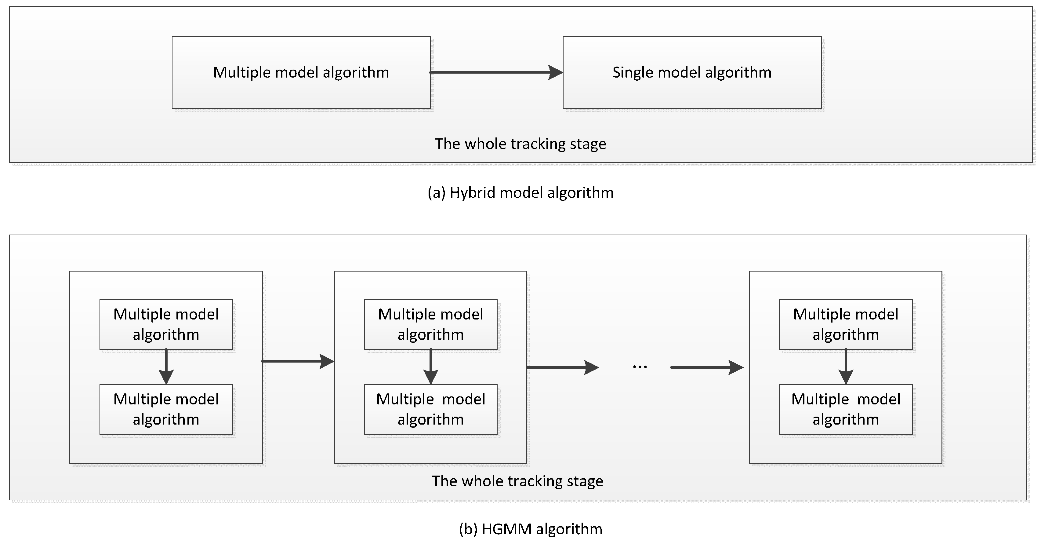
3.3. Hybrid Model Algorithm

We are stimulated by the idea of a hybrid grid multiple model (HGMM) [16] algorithm and we propose an absolutely improved algorithm called the hybrid model algorithm. The model set in effect in the HGMM algorithm consists of two types of model subsets: a fixed coarse grid and an adaptive fine grid. The coarse subset is obtained by quantizing the mode space crudely and the fine subset is designed from the region surrounding the optimal estimate of the true mode. One cycle of HGMM consists of three steps: the first step is to obtain the mode estimate based on the fixed coarse grid; the second step is to design the fine grid using the mode estimate; third step is to run the variable structure–interacting multiple model algorithm. The hybrid model algorithm is not hybrid in every recursion like the HGMM algorithm but it is hybrid in the whole filtering stage (the initial filtering stage and the stable filtering stage). The differences between the hybrid model algorithm and the HGMM algorithm are shown in Figure 1.

From Figure 1 we can know that the hybrid model algorithm is a hybrid of the multiple model algorithm and the single model algorithm in the whole tracking stage, but the HGMM algorithm includes many hybrids from the coarse grid and fine grid in the whole tracking stage.

To solve the problem of big errors in the initial tracking stage using the single model algorithm because of the uncertain initial state and in the stable tracking stage using the multiple model algorithm because of the excessive “competition” from the “unnecessary” models, we develop the hybrid model algorithm with multiple models in the initial tracking stage and a single model in the stable tracking stage. The turning point from the multiple model algorithm to the single model algorithm is an approximate time denoted as

$$f=\frac{V}{\sqrt[2]{{\left(R_0{\sigma }_{\mathrm{A}}\right)}^2+{\left(R_0{\sigma }_E\right)}^2+{\sigma }_R^2}}$$

(10)

$$t_s=fT$$

(11)

where ${\sigma }_{\mathrm{A}},{\sigma }_E,{\sigma }_{\mathrm{R}}$ and $R_0$ have been defined as parameters of the radar measurement in Section 2.2, respectively. T is the time interval for the Kalman filter recursion. The HGV tracking system enters into the stable tracking stage after the f-th Kalman filter recursion.

More specifically, we use the multiple model algorithm before time $t_s$ and use the single model algorithm after time $t_s$. The tracking performance can be improved using the multiple model algorithm when the initial state is unknown in the initial tracking stage, and the tracking performance is better using the single model algorithm in the stable tracking stage.

4. Simulation Results

In this section, two representative scenarios will be generated as HGV maneuvering trajectories and tracked using the above three algorithms. In order to make the simulation results objective and practical, we choose the average values of the variation ranges of the two control variables as the initial states.

We generate the HGV trajectory using the following initial augmented state: $V=6000$ m/s; $\theta =-5.73°$; $\sigma =0°$; $r=6.378\times {10}^6+50\times {10}^3$ m; $\lambda =0^{\circ }$; $\varphi =0^{\circ }$. Furthermore, the HGV makes skipping longitudinally flight at the fixed AOA ${10}^{\circ }$. To validate the effectiveness of the HGV maneuvering trajectory tracking algorithms proposed in this paper, two lateral maneuvering methods are given from

$$\{\begin{array}{c}\begin{array}{c}\nu ={20}^{\circ },V>V_1\\ \nu =0^{\circ },V_2<V<V_1\end{array}\\ \nu =-{20}^{\circ },V<V_2\end{array}$$

(12)

$$\nu =20\sin \left(t\pi /40\right)$$

(13)

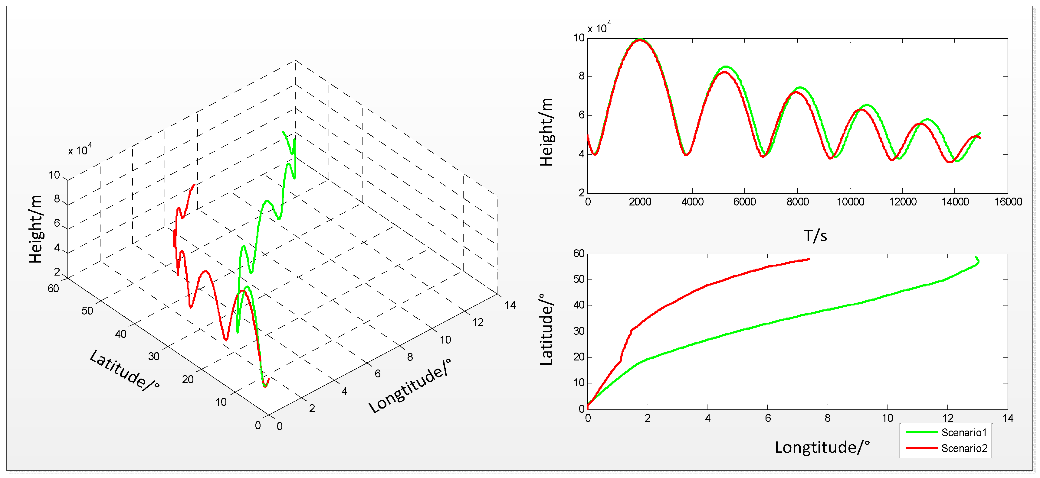
where $V_1$ = 5000 m/s and $V_2$ = 4500 m/s; t denotes the flight time. Equation (12) shows the HGV maneuvers laterally at the biggest degree. Equation (13) shows the HGV maneuvers laterally with the bank angle changing in the sine law with a period of 80 s and an amplitude of 20°. Then two HGV trajectory scenarios can be generated as shown in Figure 2.

In Figure 2, scenario 1 is generated based on Equation (12) and scenario 2 is generated based on Equation (13). From Figure 2 we can know that the HGV maneuvers laterally more strongly when the bank angle changes according to Equation (12).

We set that the radar is located at the position: $r=6.378\times {10}^6+200 \mathrm{m}$; $\lambda =-5.625°$; $\varphi =11.25°$. The standard deviation of the radar measurement errors is set as

$$\left[\begin{array}{ccc}{\sigma }_R& {\sigma }_A& {\sigma }_E\end{array}\right]=\left[\begin{array}{ccc}10 \mathrm{m}& 0.0286°& 0.0286°\end{array}\right]$$

(14)

Every process noise covariance matrix in all tracking models is set as

$$Q=diag\left(\left[5^2,{0.0573}^2,{0.0573}^2,{50}^2,{0.000573}^2,{0.000573}^2,{0.01}^2,{0.01}^2\right]\right)$$

(15)

In the algorithm simulation, the time interval T is 0.1 s. In addition, the initial state for all HGV tracking algorithms is set as

$$X_0=\left[\begin{array}{cccccccc}6000& -5.73& 0& (6.378\times {10}^6+50\times {10}^3)& 0& 0& 9& 0\end{array}\right]$$

(16)

Based on the set about the radar and the initial state, the turning point from the multiple model algorithm to the single model algorithm is approximately $t_s=17.9$s. So we use approximately $t_s=20$s in the hybrid model algorithm for HGV tracking.

The model switching probability ${\rho }_{ij}$ for the multiple model algorithm is a constant matrix with a large value on the diagonal elements. The nine-model switching probability for the nine-model IMM algorithm can be set as

$${\rho }_{ij}=\{\begin{array}{c}0.6,i=j\\ 0.05,i\ne j\end{array}$$

(17)

The initial model probability for the nine-model tracking algorithm is taken assuming the first model is near to the real model of the HGV, that is:

$${\omega }_0^j=\{\begin{array}{c}0.2,j=1\\ 0.1,\mathrm{otherwise}\end{array}$$

(18)

Then we can conduct HGV tracking using the three algorithms mentioned above and run 100 Monte-Carlo simulations for every algorithm on each trajectory. We use the root mean square error (RMSE) of the position and velocity to contrast the performances of the different tracking algorithms. The RMSE, average RMSE (ARMSE) and peak RMSE (PRMSE) can be defined as

$$RMSE\left(k\right)=\sqrt{\frac{1}{n_{MC}}{\displaystyle \sum _{i=1}^{n_{MC}}{\left({\widehat{X}}_{k/k}^{(i)}-X_k\right)}^2}}$$

(19)

$$ARMSE=\frac{1}{m}{\displaystyle \sum _{k=n}^{n+m}RMSE(k)}$$

(20)

$$PRMSE=\underset{n\le k\le m+n}{\max }(RMSE(k))$$

(21)

where $n_{MC}=100$ is the Monte-Carlo simulation number; ${\widehat{X}}_{k/k}^{(i)}$ is the predicted state at discrete time k at the i-th Monte-Carlo simulation; $X_k$ is the real state at discrete time k.

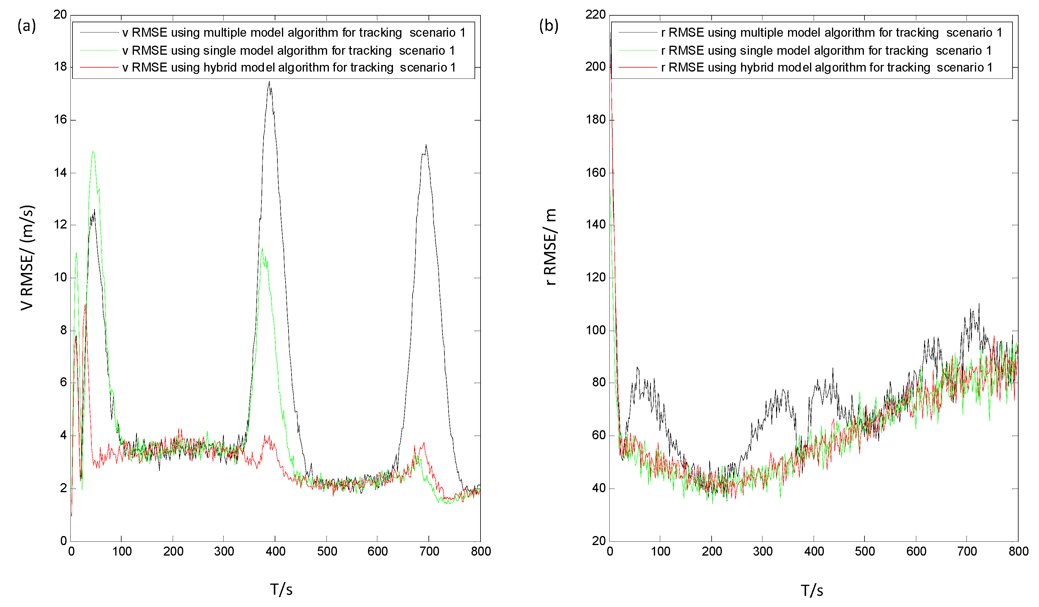
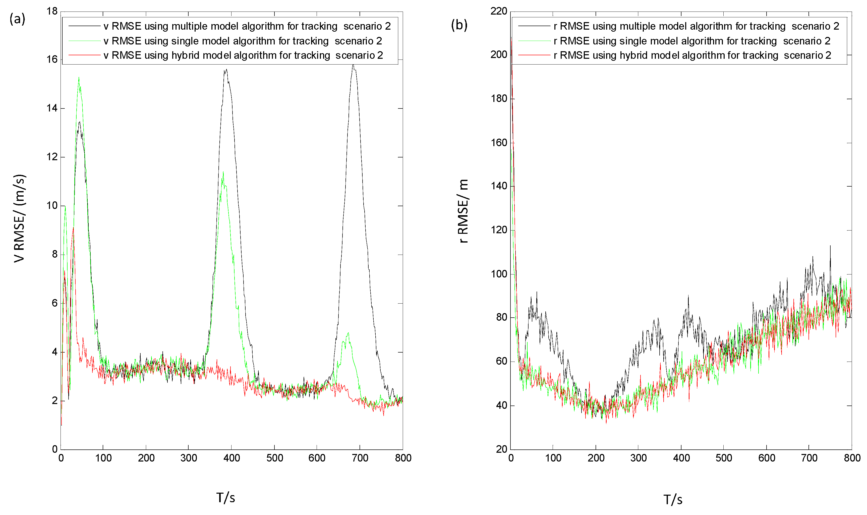
The RMSE of r and V using different algorithms in scenarios 1 and 2 are shown as Figure 3 and Figure 4, respectively. The ARMSE and PRMSE of r and V using different algorithms in scenarios 1 and 2 are shown in

Table 1. The performances for tracking scenario 1, ARMSE: average root mean square error; PRMSE: peak root mean square error.

Algorithm	V ARMSE (m/s)	V PRMSE (m/s)	r ARMSE (m)	r PRMSE (m)
Multiple model	5.30	17.96	74.18	214.09
Single model	3.89	15.33	61.36	164.95
Hybrid model	2.95	9.49	62.34	217.18

and

Table 2. The performances for tracking scenario 2.

Algorithm	V ARMSE (m/s)	V PRMSE (m/s)	r ARMSE (m)	r PRMSE (m)
Multiple model	5.29	16.26	70.87	219.16
Single model	4.04	15.69	59.70	161.32
Hybrid model	2.91	9.88	60.63	214.73

, respectively.

5. Discussion

From Table 1 and Table 2 we can see that the hybrid model algorithm has the best V ARMSE and V PRMSE in these algorithms, because the fixed coarse grid (multiple model) is good for reducing the V RMSE caused by the uncertain initial control variables and the fine grid (single model) is good for reducing the V RMSE caused by excessive “competition” from the “unnecessary” models in the stable tracking stage.

However, the r ARMSE using the hybrid model algorithm is a bit higher than that using the single model algorithm and the r PRMSE using the hybrid model algorithm is about the same as that using the multiple model algorithm. In the initial tracking stage, using the multiple model results in a bigger r RMSE because it is slow that the changes of the speed propagate to that of the position in a nonlinear system with excessive models, and the fixed coarse grid does not come into effect in the initial tracking stage.

The higher r PRMSE using the hybrid model algorithm is caused by the multiple model algorithm in the initial tracking stage. The r ARMSE using the hybrid model algorithm is about 1.6% greater than that using the single model algorithm. However, the V RMSE using the single model algorithm is about 30% greater than that using the hybrid model algorithm.

The numbers of the model filters mainly determine the computational cost of the HGV tracking algorithm. There is only one model filter in the single model algorithm and there are nine model filters in the multiple model algorithm. Obviously, the computational cost of the hybrid model algorithm is slightly higher than that of the single model algorithm but much lower than that of the multiple model algorithm. It is acceptable that the V accuracy is improved significantly with the slightly higher computational cost.

In a system for defending HGVs we take more consideration of the speed accuracy in the whole tracking stage and the position accuracy in the stable tracking stage, because we need to launch the interceptor missile in the stable tracking stage and the speed accuracy has more effect on the trajectory prediction as time goes on. From Figure 3 and Figure 4, we can know that the V RMSE and r RMSE using the hybrid algorithm are quick to converge. The hybrid model algorithm has the lowest V RMSE in these algorithms and about the same r RMSE as the single model algorithm. Thus, the hybrid model algorithm is the best choice for HGV tracking of the three algorithms.

The hybrid model algorithm may be promising for some general-maneuvering target tracking, which will be studied in future research.

References

- Li, G.; Zhang, H.; Tang, G.; Xie, Y. Maneuver modes analysis for hypersonic glide vehicles. Guid. Navig. Control Conf. 2014, 43, 543–548. [Google Scholar]
- Zhang, X.Y.; Wang, G.H.; Song, Z.Y.; Gu, J.J. Hypersonic sliding target tracking in near space. Def. Technol. 2015, 29, 370–381. [Google Scholar] [CrossRef]
- Qin, L.J.; Zhou, D. Tracking filter algorithm for near space target based on AGIMM. Syst. Eng. Electr. 2015, 37, 1009–1014. [Google Scholar]
- Wang, H.; Liu, G.; Gu, X. Research on adaptive turning model in grid multiple model algorithm. J. Proj. Rocket. Missiles Guid. 2008, 28, 241–244. [Google Scholar]
- Wu, W.; Pan, Q.; Zhao, C.; Liu, L. A probability hypothesis density filter with singer model for maneuver target tracking. In Proceedings of the 2013 32nd Chinese Control Conference (CCC), Xi’an, China, 26–28 July 2013.
- Zhai, D.; Lei, H.; Li, J.; Liu, T. Trajectory prediction of hypersonic vehicles based on the self-adaptive IMM. Acta Aeronaut. Astronaut. Sin. 2016, 37, 245–253. [Google Scholar]
- Fan, Y.; Zhu, W.; Bai, G. A Cost-Effective Tracking algorithm for hypersonic glide vehicle maneuver based on modified aerodynamic model. Appl. Sci. 2016, 6, 312. [Google Scholar] [CrossRef]
- Arasaratnam, I.; Haykin, S. Cubature kalman filters. IEEE Trans. Autom. Control 2009, 54, 1254–1269. [Google Scholar] [CrossRef]
- Aidala, V.J. Kalman filter behavior in bearings-only tracking applications. IEEE Trans. Aerosp. Electr. Syst. 1979, 15, 29–39. [Google Scholar] [CrossRef]
- Julier, S.J.; Uhlmann, J.K.; Durrant-Whyte, H.F. A new approach for filtering nonlinear systems. Am. Control Conf. 1995, 3, 1628–1632. [Google Scholar]
- Zhu, W.; Wang, W.; Yuan, G. An improved interacting multiple model filtering algorithm based on the cubature kalman filter for maneuvering target tracking. Sensors 2016, 16, 805. [Google Scholar] [CrossRef] [PubMed]
- Ho, Y.-C.; Lee, R. A Bayesian approach to problems in stochastic estimation and control. IEEE Trans. Autom. Control 1964, 9, 333–339. [Google Scholar] [CrossRef]
- Shen, Z.; Lu, P. Dynamic lateral entry guidance logic. J. Guid. Control Dyn. 2004, 27, 949–959. [Google Scholar] [CrossRef]
- Ding, L.; Geng, F.; Chen, J. Radar Principle; Publishing House of Electronics Industry: Beijing, China, 2009. [Google Scholar]
- Blom, H.A.P.; Barshalom, Y. The interacting multiple model algorithm for systems with Markovian switching coefficients. IEEE Trans. Autom. Control 1988, 33, 780–783. [Google Scholar] [CrossRef]
- Xu, L.; Li, X.R.; Duan, Z. Hybrid grid multiple-model estimation with application to maneuvering target tracking. IEEE Trans. Aerosp. Electr. Syst. 2016, 52, 122–136. [Google Scholar] [CrossRef]
© 2017 by the authors. Licensee MDPI, Basel, Switzerland. This article is an open access article distributed under the terms and conditions of the Creative Commons Attribution (CC BY) license ( http://creativecommons.org/licenses/by/4.0/).