Light Trapping above the Light Cone in One-Dimensional Arrays of Dielectric Spheres

Abstract

We demonstrate bound states in the radiation continuum (BSC) in a linear periodic array of dielectric spheres in air above the light cone. We classify the BSCs by orbital angular momentum $m=0,\pm 1,\pm 2$ according to the rotational symmetry of the array, Bloch wave vector β directed along the array according to the translational symmetry, and polarization. The most simple symmetry protected BSCs have $m=0,\beta =0$ and occur in a wide range of the radius of the spheres and dielectric constant. More sophisticated BSCs with $m\ne 0,\beta =0$ exist only for a selected radius of spheres at fixed dielectric constant. We also find robust Bloch BSCs with $\beta \ne 0,m=0$. All BSCs reside within the first but below the other diffraction continua. We show that the BSCs can be easily detected by bright features in scattering of different plane waves by the array as dependent on type of the BSC. The symmetry protected TE/TM BSCs can be traced by collapsing Fano resonance in cross-sections of normally incident TE/TM plane waves. When plane wave with circular polarization with frequency tuned to the bound states with OAM illuminates the array the spin angular momentum of the incident wave transfers into the orbital angular momentum of the BSC. This, in turn, gives rise to giant vortical power currents rotating around the array. Incident wave with linear polarization with frequency tuned to the Bloch bound state in the continuum induces giant laminar power currents. At last, the plane wave with linear polarization incident under tilt relative to the axis of array excites Poynting currents spiralling around the array. It is demonstrated numerically that quasi-bound leaky modes of the array can propagate both stationary waves and light pulses to a distance of 60 wavelengths at the frequencies close to the bound states in the radiation continuum. A semi-analytical estimate for decay rates of the guided waves is found to match the numerical data to a good accuracy.

1. Introduction

The scattering of electromagnetic waves by an ensemble of dielectric spheres has a long history of research beginning with Mie who presented a rigorous theory for scattering by a single dielectric sphere [1]. The overwhelming majority of papers since the pioneering papers by Ohtaka and his coauthors [2,3,4] considered the periodical two- and three-dimensional arrays [5,6,7,8]. Surprisingly, less interest has been payed to scattering by a linear array of dielectric nanoparticles mostly restricted to aggregates of a finite number of spheres [9,10,11]. Guiding of electromagnetic waves by a linear array of dielectric spheres below the diffraction limit attracted more attention. There were two types of consideration: finite arrays [12,13,14,15,16] and infinite arrays which were studied by means of the coupled-dipole approximation [17,18,19,20,21,22,23]. Only in 2013 a full-wave analysis of waves on linear arrays of dielectric spheres below the light cone was provided by Linton, Zalipaev, and Thompson [24]. It has been widely believed that only those modes whose eigenfrequencies lie below the light cone, are confined and the rest of the eigenmodes have finite life times. However recently confined electromagnetic modes were shown to exist in various periodical arrays of:

(i)

long cylindrical rods [25,26,27,28,29,30,31,32,33,34,35,36,37,38,39,40,41,42,43]

(ii)

photonic crystal slabs [44,45,46,47,48,49,50,51] and

(iii)

two-dimensional arrays of spheres [40,52].

Surprisingly, less attention is paid to the one-dimensional array of dielectric nanoparticles. Similar one may expect light trapping in the one-dimensional array of nanoparticles with the bound frequencies above the light cone. The array of dielectric spheres or discs is interesting due to the rotational symmetry giving rise to that the orbital angular momentum (OAM) of light is preserved. Therefore one can expect the the BSCs with non-zero OAM. The angular momentum is composed of the spin angular momentum (SAM) and OAM describing the polarization and the phase structure distribution of EM fields, respectively [53,54,55]. In this review we summarize our resent results on BSCs in arrays of dielectric spheres [56] including some findings on transport properties of dielectric arrays [57] and BSCs with OAM [58,59]. For a thorough review of BSCs the reader is addressed to [60].

2. Basic Equations for EM Wave Scattering by a Linear Array of Spheres

In the present paper we consider a free-standing one-dimensional infinite array of dielectric spheres in air Figure 1. In what follows we refer all length quantities in terms of the period h of the array.

We formulate the scattering theory by a periodic array of dielectric spheres in the form similar to the approach developed for a periodic array of dielectric cylinders [37,61]

$${\widehat{S}}^{-1}\mathrm{\Psi }=\widehat{L}\mathrm{\Psi }={\mathrm{\Psi }}_{inc}.$$

(1)

where the matrix $\widehat{L}$ accounts for both the scattering matrix of the isolated sphere as well as the mutual scattering events between the spheres, ${\mathrm{\Psi }}_{inc}$ is given by the incident wave, and the column Ψ consists of amplitudes $a_l^m$ of the multipole expansion of the scattering function.

The exact expression of the matrix $\widehat{L}$ was derived by Linton et al. [24] for EM guided waves on a periodic array of dielectric spheres. For the reader’s convenience we present the equations and notations from the above reference. We seek the solutions of the Maxwell equations, which obey the Bloch theorem:

$$\mathbf{E}(\mathbf{r}+{\mathbf{R}}_j)=e^{i\beta j}\mathbf{E}\left(\mathbf{r}\right),\mathbf{H}(\mathbf{r}+{\mathbf{R}}_j)=e^{i\beta j}\mathbf{H}\left(\mathbf{r}\right)$$

with the Bloch wave vector β directed along the array aligned with the z-axis (see Figure 1). Here ${\mathbf{R}}_j=j{\mathbf{e}}_z$ is the position of the center of the j-th sphere and ${\mathbf{e}}_z$ is the unit vector along the array. Scattered electromagnetic fields are expanded in a series over vector spherical harmonics ${\mathbf{M}}_n^m$ and ${\mathbf{N}}_n^m$ [1,24].

$$\begin{array}{c}\mathbf{E}\left(\mathbf{r}\right)={\sum }_j{e}^{i\beta j}{\sum }_{lm}[a_l^m{\mathbf{M}}_l^m(\mathbf{r}-{\mathbf{R}}_j)+b_l^m{\mathbf{N}}_l^m(\mathbf{r}-{\mathbf{R}}_j)],\\ \mathbf{H}\left(\mathbf{r}\right)=-i{\sum }_j{e}^{i\beta j}{\sum }_{lm}[a_l^m{\mathbf{N}}_l^m(\mathbf{r}-{\mathbf{R}}_j)+b_l^m{\mathbf{M}}_l^m(\mathbf{r}-{\mathbf{R}}_j)].\end{array}$$

(2)

In series (2) the first/second terms presents TE/TM spherical vector EM fields.

In absence of an incident wave Linton et al. [24] derived the homogeneous matrix equation for the amplitudes $a_l^m,b_l^m$.

$$\begin{array}{c}{Z}_{TE,l}^{-1}{a}_l^m-{\sum }_{\nu }(a_{\nu }^m{\mathcal{A}}_{\nu l}^{mm}+b_{\nu }^m{\mathcal{B}}_{\nu l}^{mm})=0,\\ Z_{TM,l}^{-1}{b}_l^m-{\sum }_{\nu }(a_{\nu }^m{\mathcal{B}}_{\nu l}^{mm}+b_{\nu }^m{\mathcal{A}}_{\nu l}^{mm})=0,\end{array}$$

(3)

where summation over ν begins with $max(1,m)$, and the so-called Lorenz-Mie coefficients are given by

$$\begin{array}{ccc}\hfill & Z_{TE,l}=\frac{j_l\left(kR\right){\left[r{j}_l\left(k_{0}r\right)\right]}_{r=R}^{\prime }-j_l\left(k_{0}R\right){\left[r{j}_l\left(kr\right)\right]}_{r=R}^{\prime }}{h_l\left(k_{0}R\right){\left[r{j}_l\left(kr\right)\right]}_{r=R}^{\prime }-j_l\left(kR\right){\left[r{h}_l\left(k_{0}r\right)\right]}_{r=R}^{\prime }},& \hfill \\ & Z_{TM,l}=\frac{ϵj_l\left(kR\right){\left[r{j}_l\left(k_{0}r\right)\right]}_{r=R}^{\prime }-j_l\left(k_{0}R\right){\left[r{j}_l\left(kr\right)\right]}_{r=R}^{\prime }}{h_l\left(k_{0}R\right){\left[r{j}_l\left(kr\right)\right]}_{r=R}^{\prime }-ϵj_l\left(kR\right){\left[r{h}_l\left(k_{0}r\right)\right]}_{r=R}^{\prime }},\end{array}$$

(4)

where $k=\sqrt{ϵ}{k}_0$ and ϵ is the dielectric constant of the spheres

$${\mathcal{A}}_{l\nu }^{mm}=4\pi {(-1)}^m{i}^{\nu -l}\sqrt{\frac{\nu (\nu +1)}{l(l+1)}}\sum _{p=|l-\nu |;l+\nu +p=even}^{l+\nu }{(-i)}^p{g}_{l\nu p}\mathcal{G}(l,m;\nu ,-m;p)s_p,$$

(5)

$${\mathcal{B}}_{l\nu }^{mm}=\frac{2\pi {(-1)}^m}{\sqrt{l(l+1)\nu (\nu +1)}}\sum _{p=|l-\nu |+1;l+\nu +p=odd}^{l+\nu -1}{i}^{\nu -l-p}\sqrt{\frac{2p+1}{2p-1}}\mathcal{H}(l,m;\nu ,-m;p)s_p.$$

(6)

The coefficients

$$g_{l\nu p}=1+\frac{(l-\nu +p+1)(l+\nu -p)}{2\nu (2\nu +1)}-\frac{(\nu -l+p+1)(l+\nu +p+2)}{2(\nu +1)(2\nu +1)},$$

(7)

$$\mathcal{G}(l,m;\nu ,\mu ;p)=\frac{{(-1)}^{m+\mu }}{\sqrt{4\pi }}\sqrt{(2l+1)(2\nu +1)(2p+1)}\left(\begin{array}{ccc}l& \nu & p\\ m& \mu & -m-\mu \end{array}\right)\left(\begin{array}{ccc}l& \nu & p\\ 0& 0& 0\end{array}\right)$$

(8)

are expressed in terms of Wigner 3-j symbols,

$$\mathcal{H}(l,m;\nu ,-m;p)=\sum _{s=-1}^1{\mathcal{G}}_s(l,m;\nu ,-m;p)$$

(9)

with

$$\begin{array}{ccc}\hfill & {\mathcal{G}}_0(l,m;\nu ,-m;p)=-2m\left|p\right|\mathcal{G}(l,m;\nu ,-m;p-1),& \hfill \\ & {\mathcal{G}}_{\pm 1}(l,m;\nu ,-m;p)=\mp \sqrt{(\nu \pm m)(\nu \mp m+1)p(p-1)}\mathcal{G}(l,m;\nu ,-m\pm 1;p-1),\end{array}$$

(10)

and

$$s_p={\lambda }_{p0}\sum _{j=1}^{\infty }{h}_p\left(k_{0}j\right)(e^{i\beta j}+{(-1)}^p{e}^{-i\beta j}),$$

(11)

where ${\lambda }_{lm}$ is normalization factor given in Appendix A. The next step is to account for an incident plane wave which can be expanded over vector spherical harmonics [1,6].

$$\begin{array}{ccc}\hfill & {\mathbf{E}}^{\sigma }\left(\mathbf{r}\right)={\sum }_{l=1}^{\infty }{\sum }_{-l}^l[q_{lm}^{\sigma }{\mathbf{M}}_l^m\left(\mathbf{r}\right)+p_{lm}^{\sigma }{\mathbf{N}}_l^m\left(\mathbf{r}\right)],& \hfill \\ & {\mathbf{H}}^{\sigma }\left(\mathbf{r}\right)=-i{\sum }_{l=1}^{\infty }{\sum }_{-l}^l[p_{lm}^{\sigma }{\mathbf{M}}_l^m\left(\mathbf{r}\right)+q_{lm}^{\sigma }{\mathbf{N}}_l^m\left(\mathbf{r}\right)].\end{array}$$

(12)

Here, index σ stands for plane TE/TM wave.

$$\begin{array}{ccc}\hfill & p_{lm}^{TE}=-F_{lm}{\tau }_{lm}\left(\alpha \right),q_{lm}^{TE}=F_{lm}{\pi }_{lm}\left(\alpha \right),& \hfill \\ & p_{lm}^{TM}=-i{F}_{lm}{\pi }_{lm}\left(\alpha \right),q_{lm}^{TM}=i{F}_{lm}{\tau }_{lm}\left(\alpha \right),\end{array}$$

(13)

$k_x=-k_0\sin \alpha ,k_y=k_0\cos \alpha$,

$$\begin{array}{ccc}\hfill & F_{lm}={(-1)}^m{i}^l\sqrt{\frac{4\pi (2l+1)(l-m)!}{(l+m)!}},& \hfill \\ & {\tau }_{lm}\left(\alpha \right)=\frac{m}{\sin \alpha }{P}_l^m\left(\cos \alpha \right),& \hfill \\ & {\pi }_{lm}\left(\alpha \right)=-\frac{d}{d\alpha }{P}_l^m\left(\cos \alpha \right).\end{array}$$

(14)

For a particular case of normal incidence $k_z=0,\alpha =-\pi /2$ we obtain from Equation (14)

$${\tau }_{lm}=-m{P}_l^m\left(0\right),{\pi }_{lm}=-\frac{d}{d\alpha }{P}_l^m\left(0\right).$$

(15)

The general equation for the amplitudes $a_l^m,b_l^m$ which describe the scattering by a linear array of spheres takes the following form:

$$\begin{array}{ccc}\hfill & Z_{TE,l}^{-1}{a}_l^m-{\sum }_{\nu }(a_{\nu }^m{\mathcal{A}}_{\nu l}^{mm}+b_{\nu }^m{\mathcal{B}}_{\nu l}^{mm})=q_{lm}^{\sigma },& \hfill \\ & Z_{TM,l}^{-1}{b}_l^m-{\sum }_{\nu }(a_{\nu }^m{\mathcal{B}}_{\nu l}^{mm}+b_{\nu }^m{\mathcal{A}}_{\nu l}^{mm})=p_{lm}^{\sigma }.\end{array}$$

(16)

Here the left hand term formulates explicitly the matrix $\widehat{L}$ in Equation (1) and the right hand term corresponds the vector of incident wave ${\mathrm{\Psi }}_{inc}$ in the space of vector spherical functions notified by two integers $l,m$ and polarization σ.

3. The Diffraction Continua of Vector Cylindrical Modes

Thanks to the axial symmetry of the array we can exploit the vector cylindrical modes for description of the diffraction continua which are doubly degenerate in TM and TE polarizations σ. The modes can be expressed through a scalar function ψ [1].

$${\psi }_{m,n}(r,\varphi ,z)=H_m^{\left(1\right)}\left({\chi }_{n}r\right)e^{im\varphi +i{k}_{z,n}z}.$$

(17)

Then for the TE modes we have

$$\begin{array}{ccc}\hfill & E_z=0,H_z={\psi }_{m,n},& \hfill \\ & E_r=\frac{i{k}_0}{{\chi }_n^2}\frac{1}{r}\frac{\partial {\psi }_{m,n}}{\partial \varphi },H_r=\frac{i{k}_z}{{\chi }_n^2}\frac{\partial {\psi }_{m,n}}{\partial r},& \hfill \\ & E_{\varphi }=\frac{-i{k}_0}{{\chi }_n^2}\frac{\partial {\psi }_{m,n}}{\partial r},H_{\varphi }=\frac{i{k}_z}{{\chi }_n^2}\frac{1}{r}\frac{\partial {\psi }_{m,n}}{\partial \varphi },\end{array}$$

(18)

and for the TM modes

$$\begin{array}{ccc}\hfill & E_z={\psi }_{m,n},H_z=0,& \hfill \\ & E_r=\frac{i{k}_z}{{\chi }_n^2}\frac{\partial {\psi }_{m,n}}{\partial r},H_r=\frac{-i{k}_0}{{\chi }_n^2}\frac{1}{r}\frac{\partial {\psi }_{m,n}}{\partial \varphi },& \hfill \\ & E_{\varphi }=\frac{i{k}_z}{{\chi }_n^2}\frac{1}{r}\frac{\partial {\psi }_{m,n}}{\partial \varphi },H_{\varphi }=\frac{i{k}_0}{{\chi }_n^2}\frac{\partial {\psi }_{m,n}}{\partial r},\end{array}$$

(19)

where

$${\chi }_n^2=k_0^2-k_{z,n}^2$$

(20)

and

$$k_{z,n}=\beta +2\pi n,n=0,\pm 1,\pm 2,\dots .$$

(21)

In what follows we consider the BSCs in the diffraction continua specified by two quantum numbers m and n where the m is the result of the axial symmetry and n is the result of translational symmetry of the infinite linear array of the dielectric spheres. Note that each diffraction continuum is doubly degenerate relative to the polarization σ. As a result of the interplay between the frequency $k_0$ and the wave number $k_{z,n}$ the continua can be open (χ is real) or closed (χ is imaginary). In the present paper we restrict ourselves by the case of one, two and three open continua.

4. Classification of BSCs in the Array of Spheres

In the previous section we presented the theory for scattering of plane waves by a periodic array of dielectric spheres based on the approach by Linton et al. [24]. If there is no incident wave we have $\widehat{L}\mathbf{a}=0$ whose solutions are bound modes of the array. There might be two kinds of the bound modes. The first type of modes have wave number $\beta >k_0$ and describe guided waves along the array. These solutions found by Linton et al. exist in some interval of the material parameters of spheres, dielectric constant ϵ or radius R, and the Bloch wave number β [24]. The second type of bound modes with $\beta <k_0$ resides above the light cone (BSCs). It is much more difficult to establish the existence of the second type of bound states because a tuning of material parameters is required. However there might exist symmetry protected BSCs which are robust with respect to the material parameters. These BSCs have been already considered in the linear array of infinitely long dielectric rods [31,33,35,37,40,41,42,43,44,45].

The axial symmetry of the array implies that the matrices $\mathcal{A}$ and $\mathcal{B}$ split into the irreducible representations of the azimuthal number m which therefore classifies the BSCs. Next, the discrete translational symmetry along the z-axis implies that the respective wave number β specifies the BSC. At last, additional optional symmetries arise due to the inversion symmetry transformation $\widehat{K}f(x,y,z)=f(x,y,-z)$ for $\beta =0,\pi$. It follows from Equation (11) that $s_{2k+1}=0$, and respectively from Equations (5) and (60) we obtain ${\mathcal{A}}_{\nu L}^{mm}=0$ if $l+\nu$ is odd, and ${\mathcal{B}}_{\nu L}^{mm}=0$ if $l+\nu$ is even. Moreover for arbitrary β: ${\mathcal{B}}_{\nu l}^{00}=0$ (see Appendix A). These relations establish the selection rules for the amplitudes $a_l^m,b_l^m$ which determine allowed BSC modes listed in the

Table 1. Classification of the bound states in the radiation continuum (BSCs).

m	β	Type I of BSC	Type II of BSC
$\ne 0$	0	$(a_{2k}^m,b_{2k+1}^m)$	$(a_{2k+1}^m,b_{2k}^m)$
0	$\ne 0$	$(a_l^0,0),E_z=0$	$(0,b_l^0),H_z=0$
0	0	$(a_{2k}^0,0),E_z=0$	$(0,b_{2k}^0),H_z=0$
0	0	$(0,b_{2k+1}^0),H_z=0$	$(a_{2k+1}^0,0),E_z=0$

.

The cartesian components of the vector spherical functions transform under the inversion of z as follows

$$\begin{array}{ccc}\hfill & M_{l,x,y}^m(\pi -\theta )=-{(-1)}^{l-m}{M}_{l,x,y}^m\left(\theta \right),M_{l,z}^m(\pi -\theta )={(-1)}^{l-m}{M}_{l,z}^m\left(\theta \right),& \hfill \\ & N_{l,x,y}^m(\pi -\theta )={(-1)}^{l-m}{N}_{l,x,y}^m\left(\theta \right),N_{l,z}^m(\pi -\theta )=-{(-1)}^{l-m}{N}_{l,z}^m\left(\theta \right).\end{array}$$

(22)

For $\beta =0$ we have

$$\begin{array}{ccc}\hfill & {\sum }_j{M}_{l,x,y}^m(\mathbf{r}-{\mathbf{R}}_j)=-{(-1)}^{l-m}{\sum }_j{M}_{l,x,y}^m(\widehat{K}\mathbf{r}-{\mathbf{R}}_j),& \hfill \\ & {\sum }_j{M}_{l,z}^m(\mathbf{r}-{\mathbf{R}}_j)={(-1)}^{l-m}{\sum }_j{M}_{l,z}^m(\widehat{K}\mathbf{r}-{\mathbf{R}}_j).& \hfill \\ & {\sum }_j{N}_{l,x,y}^m(\mathbf{r}-{\mathbf{R}}_j)=-{(-1)}^{l-m}{\sum }_j{N}_{l,x,y}^m(\widehat{K}\mathbf{r}-{\mathbf{R}}_j),& \hfill \\ & {\sum }_j{N}_{l,z}^m(\mathbf{r}-{\mathbf{R}}_j)={(-1)}^{l-m}{\sum }_j{N}_{l,z}^m(\widehat{K}\mathbf{r}-{\mathbf{R}}_j).\end{array}$$

(23)

Then from these equations and Equation (2) one can obtain the following symmetric properties for the cartesian components of EM fields collected in

Table 2. Symmetry properties of the eigenmodes with $\beta =0$.

Type I	Type II
$E_{x,y}(-z)={(-1)}^{m+1}{E}_{x,y}\left(z\right)$	$E_{x,y}(-z)={(-1)}^m{E}_{x,y}\left(z\right)$
$E_z(-z)={(-1)}^m{E}_z\left(z\right)$	$E_z(-z)={(-1)}^{m+1}{E}_z\left(z\right)$
$H_{x,y}(-z)={(-1)}^m{H}_{x,y}\left(z\right)$	$H_{x,y}(-z)={(-1)}^{m+1}{H}_{x,y}\left(z\right)$
$H_z(-z)={(-1)}^{m+1}{H}_z\left(z\right)$	$H_z(-z)={(-1)}^m{H}_z\left(z\right)$

.

Table 1 and Table 2 will be useful for the symmetry classification of the bound modes in the next sections.

5. Symmetry Protected BSCs

In this section we present numerical solutions of Equation (3) for the symmetry protected BSCs with $m=0,\beta =0$ embedded into the first diffraction continuum $n=0$. They constitute the majority of the BSCs in the array. The symmetry protected BSCs are either pure TE spherical vector modes (Type I in Table 1) with $a_{2k}^0\ne 0,b_k^0=0$ or TM spherical vector modes (Type II in Table 1) with $a_k^0=0,b_{2k}^0\ne 0$. We show that the symmetry protected BSCs are symmetrically mismatched to the first open continuum. Below we present numerical solutions for Type I BSCs with accuracy of ${10}^{-4}$:

$$\begin{array}{c}\hfill k_0=4.24,R=0.3,ϵ=12,a_l^0=\left(\begin{array}{c}0\\ 0.7563-0.6542i\\ 0\end{array}\right),b_l^0=0,l\ge 1\end{array}$$

(24)

and for Type II as

$$\begin{array}{c}\hfill k_0=4.7504,R=0.3,ϵ=15,a_l^0=0,b_l^0=\left(\begin{array}{c}0\\ -0.6017+0.7988i\\ 0\\ 0.0004-0.0006i\end{array}\right),l\ge 1,\end{array}$$

(25)

Patterns of EM fields and EM force lines are shown in Figure 2. Hereinafter we plot only real parts of electromagnetic fields. Other patterns of the symmetry protected BSCs the reader can find in Ref. [56]. One can see from Figure 2 that in the BSC of Type I (II) electric (magnetic) force lines are parallel the sphere surface.

The symmetry protected Type I and Type II BSCs have qualitatively similar field structure with respect to $\mathbf{E}\leftrightarrow \mathbf{H}$ but are not degenerate because of different boundary conditions for $\mathbf{E}$ and $\mathbf{H}$ at the sphere surface. From Table 2 one can see why the eigenmodes (24) and (25) are protected by symmetry against decay into the diffraction continuum $m=0,n=0$. From Equations (18) and (19) we obtain that the TE/TM continuum with $k_{z,0}=0(\beta =0)$ has the only $H_z/E_z\ne 0$ independent of z. The Type I BSC has $E_z=0$ and odd $H_z$ so that these type of BSCs is symmetrically mismatched to both TE and TM continua. The Type II BSC has odd $E_z$ and $H_z=0$ to decouple from the both TE and TM continua.

Besides the fully symmetry protected BSCs from the third row in Table 1 $(a_{2k}^0,0)$ and $(0,b_{2k}^0)$, we found a partially symmetry protected Type II BSC $(a_{2k+1}^0,0)$ from the fourth row of Table 1:

$$k_0=2.934,R=0.4805,ϵ=15,a_l^0=\left(\begin{array}{c}0.6826+0.0332i\\ 0\\ -0.7291-0.0354i\\ 0\\ -0.0008\end{array}\right),b_l^0=0,l\ge 1,$$

(26)

however the Type I BSCs with $(0,b_{2k+1}^0)$ were not revealed in our computations. The BSC (26) is symmetrically mismatched relative only to the TM continuum. Zero coupling of this BSC with the TE continuum can be achieved by tuning the radius of spheres. Patterns of EM fields and EM force lines are shown in Figure 3.

5.1. $\pm m$ Degenerate BSCs with $\beta =0$

The above described mechanism for partially symmetry protected BSCs with $m=0$ can be exploited for even more complicated case $m\ne 0$. Their orbital angular momentum (OAM) $m\ne 0$ of these BSCs is the result of azimuthal rotation symmetry of the array and provide unique properties in the form of spinning or spiralling currents of the Poynting vector [58,59]. Besides, the system has the time reversal symmetry which implies that these BSCs are degenerate over $\pm m$. Let us start with the Type I BSC with $m=1$ which has the odd $E_z$ and the even $H_z$ according to Table 1 and Table 2. This BSC is symmetrically mismatched with the TM diffraction continuum $m=1,n=0$ which is independent of z. The coupling with the TE continuum can be cancelled by tuning the radius. The result of computation of this partially symmetry protected Type I BSC $(a_{2k},b_{2k+1})$ is the following

$$m=1,k_0=2.847,R=0.3945,(a_l^1,b_l^1)=\left(\begin{array}{cc}0& 0.6662+0.4273i\\ -0.33+0.5145i& 0\\ 0& -0.0048-0.0031i\\ 0& 0\end{array}\right),l\ge 1$$

(27)

and shown in Figure 4a. The Type II BSC $(a_{2k+1},b_{2k})$ with $m=2$ has even $E_z$ and odd $H_z$. It is symmetry protected against decay into the TE continuum with $m=2,n=0$ and coupling with the TM continuum is cancelled by tuning the radius with the following result

$$m=2,k_0=3.086,R=0.471,(a_l^2,b_l^2)=\left(\begin{array}{cc}0& 0.6545+0.2013i\\ -0.2142+0.6964i& 0\\ 0& -0.0057-0.0018i\\ 0& 0\\ 0& 0\end{array}\right),l\ge 2.$$

(28)

All components of electric and magnetic fields are nonzero and localized around the array as shown in Figure 4. We show the EM field around only one sphere because the pattern is periodically repeated along the z-axis. One can see that the value of OAM m reflects in the structure of force lines in the xy-plane while the number of the amplitudes $a_l^m$ reflects in the structure of lines along the z-axis.

5.2. Robust Bloch BSCs with $\beta \ne 0,m=0$

Could the Bloch BSC occur at $\beta \ne 0$ in the continuum of free-space modes? This question was first answered positively by Porter and Evans [26] who considered acoustic trapping in an array of rods of rectangular cross-section. Marinica et al. [32] demonstrated the existence of the Bloch BSC with $\beta \ne 0$ in two parallel dielectric gratings and Ndangali and Shabanov [33] in two parallel arrays of dielectric rods. In a single array of rods positioned on the surface of bulk 2d photonic crystal multiple BSCs with $\beta \ge 0$ were considered by Chia Wei Hsu et al. [44]. The Bloch BSCs in a single array of cylindrical dielectric rods in air were also reported in Refs. [37,49,62]. Such travelling wave Bloch BSCs with the eigenfrequencies above the light cone are interesting because the array serves as a waveguide although only for fixed β (see summary of BSCs in Figure 5) in contrast to the bound states below the light cone [24].

According to Table 1 the Bloch BSCs with $\beta \ne 0,m=0$ have only nonzero components $a_l^0$ or $b_l^0$. Let us first consider Type I BSCs with $b_l^0=0$ which have $E_z=0$ and, therefore, are decoupled with the TM continuum but coupled with the TE $n=0,m=0$ continuum. We show numerically that this coupling can be cancelled under variation of β. The numerical results are collected in Equation (29) below with the pattern of EM fields shown in Figure 6.

$$k_0=3.6505,R=0.4,ϵ=15,\beta =1.2074,(a_l^1,b_l^1)=\left(\begin{array}{cc}0.1053-0.0638i& 0\\ 0.1918+0.3161i& 0\\ 0.6046+0.5572i& 0\\ 0.7873+0.4777i& 0\\ -0.0033-0.0054i& 0\end{array}\right),l\ge 1.$$

(29)

Although this BSC occurs at the fixed value of β there is no necessity to tune the material parameters of the spheres and therefore the BSC can be referred to as robust which is attractive from experimental viewpoint. We managed to find only Type I BSCs for $ϵ=15$ but none of Type II. Such a difference between the types is related to different boundary conditions for electric and magnetic fields at material interfaces. We collected all BSCs in Figure 5.

6. Light Guiding above the Light Line

The arrays of dielectric nanonparticles can serve as subwavelength waveguides to be emploied as the key components for future integrated optics [15,16,17,18,19,21]. They could be potentially advantageous against nanoplasmonics due to, for instance, the opportunity to control the frequencies of electric and magnetic Mie resonances by changing the geometry of high-index nanoparticles, and the absence of free carriers resulting in a high Q-factor. Arguably, the arrays of dielectric nanoparticles provide one of the most promising subwavelength set-ups for efficient light guiding [16,22] as well as more intricate effects such as resonant transmission of light [22], and optical nanoantennas [23].

So far the major theoretical tool for analyzing the infinite arrays of spherical dielectric nanoparticles has been the coupled-dipole approximation [63,64,65]. In that approximation guided waves in arrays of magnetodielectric spheres were first considered by Shore and Yaghjian [66,67] who derived the dispersion relation and computed the dispersion curves for dipolar waves. Recently a more tractable form of the dispersion equations was presented by the same authors [68] with the use of the polilogarithmic functions. The dipolar waves in arrays of Si dielectric nanospheres were thoroughly analyzed in [21]. It was shown that only two lowest guided modes could be fairly described by the dipole approximation which breaks down as the frequency approaches the first quadruple Mie resonance. This limits the application of the dipolar dispersion diagrams to realistic waveguides assembled of dielectric nanoparticles. As an alternative to the dipole approximation a “semiclassical” approach based on the coupling of the whispering gallery modes of individual spheres could be employed to recover the array band structure [69,70] if the wavelength is much smaller than the diameter of the spheres. The general case, however, requires a full-wave Mie scattering approach to account for all possible multipole resonances [19] involving a very complicated multiscattering picture which mathematically manifests itself in infinite multipole sums. Luckily, such an approach was recently developed by Linton, Zalipaev, and Thompson who managed to obtain a multipole dispersion relation in a closed form suitable for numerical computations [24]. The above approach was used for analyzing the spectra of dielectric arrays above the line of light in Ref. [56]. It was demonstrated that under variation of some parameter such as, for example, the radius of the spheres the leaky modes dominating the spectrum can acquire an infinite life-time. In other words, the array can support bound states in the radiation continuum (BSCs) [33,35,37,48,71]. In this letter, we will address the ability of the BSCs to propagate light along the array primarily motivated by finding new opportunities for designing subwavelength waveguides.

The dispersion diagram of an array of dielectric nanoparticles was obtained [57]. The dispersion curves were computed by solving the dispersion equations $f_{d,m}(k,\beta )=0$, where k is the vacuum wave number $k=\omega /c$, and β is the Bloch wave number, while the subscripts $d,m$ designate either dipole [21,68], or multipole [24] dispersion relations. For brevity we do not present the exact dispersion relations $f_{d,m}(k,\beta )=0$. A mathematically inquisitive reader is referred to the above cited papers to examine the rather cumbersome expressions for $f_{d,m}(k,\beta )$. Here we assume that the array consists of spherical noanoparticles of radius R with dielectric constant $ϵ=15$ (Si) in vacuum. The centers of the nanoparticles are separated by distance a. It is worth mentioning that at a given dielectric constant the dispersion is only dependent on a single dimensionless quantity $R/a$. This allowed to scale the model for a microwave experiment [21]. There are three types of dipolar solutions [21], namely; longitudinal magnetic (LM), longitudinal electric (LE), and transverse electromagnetic (TEM) waves. In Figure 7 we plot the lowest frequency modes of each type in comparison against the multipole solution [24]. In all cases if the $k-\beta$ curve is above the light line $k=\beta$ the vacuum wave number becomes complex valued. The imaginary part of k is linked to the mode life-time through the following formula:

$$\tau =-{\left[c\Im \left(k\right)\right]}^{-1}.$$

(30)

Two approaches are possible for description of the leaky modes; complex frequency ω [61,72], or complex Bloch number β [21,73]. In the latter case the inverse of the imaginary part of β is the penetration depth into the array $L_{\tau }={\left[\Im \left(\beta \right)\right]}^{-1}$. The quantities τ and $L_{\tau }$ are, in fact, proportional

$$L_{\tau }=v\tau ,$$

(31)

where v is the group velocity $v=d\Re \left(\omega \right)/d\beta$. Here, we do not present the imaginary part of β mentioning in passing that the penetration depths for dipolar waves were analyzed in refs. [21,73]. What is important the numerical data available so far [21,56,73] indicate that all dipolar leaky modes are relatively short-lived, in particular, no dipolar BSCs were found in Ref. [56]. In compliance with Ref. [21] Figure 7 demonstrates that only two lowest eigenmodes are fairly described by the dipole approximation.

Now, let us consider the multipolar quasi-guided modes within the first radiation continuum [56]. The dispersion curves for a leaky mode for two different ratios $R/a$ are plotted in Figure 8a. One can see that in contrast to the dipolar waves in Figure 7 now the solutions could be long-lived with the life-time Equation (30) growing up to infinity at the BSC points. It should pointed out that for both $R/a$ of all leaky modes of the array we plot only one which has a Bloch BSC point $\Im \left(k\right)=0$ at $\beta \ne 0$. As shown in Figure 8b the BSC exists in a wide range of parameter $R/a$. The magnetic and electric vectors could be found in terms of Mie coefficients $a_n^m,b_n^m$. For instance, outside the spheres one has for the electric vector $\mathbf{E}\left(\mathbf{r}\right)$ [24]

$$\mathbf{E}\left(\mathbf{r}\right)=\sum _{j=-\infty }^{\infty }{e}^{iaj\beta }\sum _{n=m^{*}}^{\infty }\left[a_n^m{\mathbf{M}}_n^m(\mathbf{r}-{\mathbf{r}}_j)+b_n^m{\mathbf{N}}_n^m(\mathbf{r}-{\mathbf{r}}_j)\right],$$

(32)

where j the number of the particle in the array, m - azimuthal number, $m^{*}=max(1,m)$, and ${\mathbf{N}}_n^m\left(\mathbf{r}\right),{\mathbf{M}}_n^m\left(\mathbf{r}\right)$ are spherical vector harmonics [1]. Only $m=0$ Bloch BSCs were found in Ref. [56]. Our numerics indicate that for BSCs in Figure 8 the dominating term in the expansions (32) corresponds to coefficient $a_3^0$. In the insets in Figure 8b we plot the components of the electric and magnetic vectors of the BSC solution. One can see that the electromagnetic field is localized in the vicinity of the array. The amplitude of a wave propagating along the array attenuates exponentially according to a simple formula

$$F\left(x\right)=e^{-x/L_{\tau }},$$

(33)

where $x=ja$ is the distance. In the vicinity of a BSC the $\omega -\beta$ dependance could be approximated as

$$\omega -{\omega }_0=v_0(\beta -{\beta }_0)+\mathcal{O}\left[{(\beta -{\beta }_0)}^2\right],$$

(34)

where ${\omega }_0,{\beta }_0,v_0$ are the BSC eigenfrequency, Bloch number, and group velocity, correspondingly.

$$-\Im \left\{k\right\}=\alpha {(\beta -{\beta }_0)}^2+\mathcal{O}\left[{(\beta -{\beta }_0)}^3\right].$$

(35)

Combining Equations (30), (31) and (33)–(35) one obtains in the vicinity of a BSC

$$F\left(x\right)=\exp \left[-\frac{\alpha xc}{v_0^3}{(\omega -{\omega }_0)}^2\right].$$

(36)

Thus, for the width of the transparency window in the frequency domain we have

$$\Delta \left(x\right)=\sqrt{\frac{v_0^3}{\alpha c}}\frac{1}{\sqrt{x}}$$

(37)

with α and $v_0$ extracted from the data in Figure 8 by a polynomial fit. Nevertheless, care is needed in applying Equation (36) as the frequency may fall out of the range where the dispersion is well approximated by the leading terms in Equations (34) and (35).

Using a full-wave multiscattering method [19] we simulated wave propagation in a finite array of 400 nanoparticles. In our numerical experiment a linearly polarized Gaussian beam [74] with the Rayleigh range $z_0=5a$ was focused on the first nanoparticle in the array. The wave vector of the beam was directed along the y-axis perpendicular to the array (see Figure 7), and the magnetic vector aligned with the array axis. In Figure 9a we plot the the leading Mie coefficient $a_3^0$ for the last nanoparticle in the array. The result shows a pronounced resonant behavior due to formation of standing waves as a consequence of the finiteness of the array. The distance between the resonances $\Delta \omega$ could be assessed as $\Delta \omega \approx \pi v_0/\left(aN\right)$ where N is the number of particles in the array. The resonant features could be averaged out by integration over small frequency intervals larger than $\Delta \omega$. The result is shown in Figure 9a in comparison against Equation (36). One can see that Equation (36) matches the numerical data to a good accuracy. The finiteness of chain also results in additional attenuation due to the radiative losses at the ends of the array. A detailed study of that effect was undertaken in Ref. [19] where it was shown that the Q factor of the finite arrays of high index nanoparticles scales as $C{N}^3$ with $0.1<C<10$ which makes such radiative losses negligible for $N=400$. The discrepancy in Figure 9 is due to the higher order terms in Equations (34) and (35).

Finally, pulse propagation along the array was considered in the above set-up with a continuous superposition of Gaussian beams forming a Gaussian light pulse of width ${\sigma }_{\omega }$ in the frequency domain. The central wave number of the pulse was adjusted to the BSC wave number $k_0=\pi 1.162/a$. At the moment $t=0$ a light pulse was injected into the left end of the array. In Figure 9b we plot four snapshots of the leading Mie coefficient $a_3^0$ against the distance along the array for three different initial pulse widths ${\sigma }_{\omega }$. One can clearly see in Figure 9b that the pulse propagating along the array tends to spread as the harmonics distant in the ω-space from the BSC frequency decay into the continuum. The pulse profile $f(x,t)$ could be found by Fourier-transforming the initial Gaussian pulse to the real space:

$$f(x,t)=\frac{1}{\sigma \left(t\right)}{e}^{-\frac{{(x-v_{0}t)}^2}{{\sigma }^2\left(t\right)}}{e}^{i({\beta }_{0}x-{\omega }_{0}t)}$$

(38)

with

$${\sigma }^2\left(t\right)=4a^2\left[{\left(\frac{v_0}{a{\sigma }_{\omega }}\right)}^2+\frac{c\alpha }{a^2}t\right].$$

(39)

Analyzing Equation (39) for a given distance $L=v_{0}t$ one can identify two possible regimes for the pulse propagation. In the "overdamped" regime the second term dominates on the left hand side of Equation (39) resulting in a noticeable spreading of the pulse in the real space. If, however, the first term dominates the pulse retains its profile during propagation time (${\sigma }_{\omega }=0.0025/t_0$ in Figure 9b). One finds from Equation (39) that the pulse doubles its width after travelling to the distance

$$L=\frac{3a^2}{\alpha }{\left(\frac{v_0}{c}\right)}^3{\left(\frac{c}{a{\sigma }_{\omega }}\right)}^2.$$

(40)

So far the material losses due to the imaginary part of the dielectric constant were neglected. Particulary in silicon the material losses vary significantly in the optical range [75]. We ran a numerical test at 725 nm with $\Im \left(ϵ\right)=0.0075$ to find that the propagation distance $L\approx 100a$, $a=421$ nm so the light can travel to approximately 60 wavelengths. It should be pointed out that in the near infrared $\lambda \approx 1000$ nm the losses can be tens of times less allowing propagation to hundreds wavelengths [21] as shown in Figure 9.

7. Emergence of the BSC in Scattering

Scattering of plane waves by periodic two-dimensional arrays of dielectric spheres originates since pioneering papers by Ohtaka et al. [3,4] (see also Ref. [5]). Scattering by aggregates of finite number of spheres was considered in the framework of multi sphere Mie scattering [6,9,11], however to our knowledge the scattering by the one-dimensional infinite array of dielectric spheres was not considered yet. The following subsections aim to present results of numerical calculation of differential and total cross-sections of the infinite array with focus to follow resonant traces of the BSCs in the cross-sections similar to the scattering by array of dielectric rods [37,44,45]. For the present case of the array of dielectric spheres we revealed different types of the BSCs. We show that excitation of corresponding quasi-BSCs needs in different ways of injection of EM waves.

The BSC has zero coupling with the continuum, i.e., the BSC has infinite quality factor [76]. Also the BSC is unique by that the solution of the scattering problem becomes ambiguous [25] and can be written as superposition of particular scattering state and the BSC [77,78].

$$\mathrm{\Psi }={\mathrm{\Psi }}_S+\alpha {\mathrm{\Psi }}_{BSC}$$

(41)

where α is arbitrary coefficient. This equation is well known mathematical consequence of the linear Lippmann-Schwinger Equation (1) when the inverse of the matrix $\widehat{L}$ does not exist, i.e., when $Det(\widehat{L})=0$. Then the BSC is the eigenmode of the matrix $\widehat{L}$

$$\widehat{L}{\mathrm{\Psi }}_{BSC}={\lambda }_c{\mathrm{\Psi }}_{BSC}$$

(42)

with real eigenvalue ${\lambda }_c$. At the first sight the BSCs are not interesting because they are invisible for probing waves incident from the continuum. However the BSC point is isolated in the parametric space and experimentalist can approach to this point only approximately. Other words, in reality we have only the quasi-BSCs whose quality factor is restricted by set-up imperfectness. Moreover for the case of arrays of dielectric rods or nanoparticles we have always finite number of them to give rise to a leakage of trapped modes into the diffraction continua. In this case the parameter α in Equation (47) is defined by the point in the parametric space. When the point is sufficiently close to the BSC point α can achieve enormous value however as dependent on the way of approaching [78]. That observation is important for applications [26,52,78,79].

According to above equation the BSC is a null eigenvector of matrix $\widehat{L}$ with zero eigenvalue. As soon as one deviates from the BSC point in the parametric space the BSC emerges in the form of a collapsing Fano resonance. That phenomenon was observed in scattering of EM waves by arrays of rods [30,33,37,40,44,45,52,62]. The Fano resonance for the present system can be interpreted as interference of two optical paths, one through the spheres and another between the spheres. In what follows we highlight these features of the BSCs using the biorthogonal basis of eigenvectors of the non-Hermitian matrix $\widehat{L}$ [37,80].

$$\widehat{L}{\mathbf{X}}_f=L_f{\mathbf{X}}_f,{\widehat{L}}^{+}{\mathbf{Y}}_f=L_f^{*}{\mathbf{Y}}_f,{\mathbf{Y}}_f^{+}{\mathbf{X}}_{f^{\prime }}={\delta }_{f{f}^{\prime }}.$$

(43)

It immediately follows that

$${\widehat{L}}^{-1}=\sum _f{\mathbf{X}}_f\frac{1}{L_f}{\mathbf{Y}}_f^{+}.$$

(44)

Because of the axial symmetry matrix $\widehat{L}$ has OAM preserving block structure

$$L_{l{l}^{\prime }}^{\left(m\right)}=\left(\begin{array}{cc}{Z}_{TE,l}^{-1}{\delta }_{l{l}^{\prime }}-{\mathcal{A}}_{l{l}^{\prime }}^{mm}& -{\mathcal{B}}_{l{l}^{\prime }}^{mm}\\ -{\mathcal{B}}_{l{l}^{\prime }}^{mm}& Z_{TM,l}^{-1}{\delta }_{l{l}^{\prime }}-{\mathcal{A}}_{l{l}^{\prime }}^{mm}\end{array}\right),$$

(45)

where each block correspond to a specific value m.

In the nearest vicinity of the BSC point one of the complex eigenvalues $L_c$ is close to zero. That allows us to substantially simplify Equation (44) leaving in the sum only the leading contribution related to $L_c$. Respectively the solution for the scattering function in Equation (1)

$$\mathrm{\Psi }={\widehat{L}}^{-1}{\mathrm{\Psi }}_{inc}$$

(46)

is simplified as follows

$${\mathrm{\Psi }}^{\sigma }\approx \frac{1}{L_c}{\mathbf{X}}_c({\mathbf{Y}}_c^{+}·{\mathrm{\Psi }}_{inc}^{\sigma }),\sigma =TE/TM.$$

(47)

This equation manifests one remarkable as well as important for applications property of the BSCs to enormously enhance the incident wave ${\mathrm{\Psi }}_{inc}$ by the factor $1/L_c$ [52,77,78].

7.1. Symmetry Protected BSCs

First the effect of enhancement of scattering function in the near zone of the infinite periodic array of dielectric spheres was shown in Ref. [56] in the vicinity to the symmetry protected BSCs with $m=0$. As it follows from Equations(20) and (21) only one diffraction channel $n=0$ is open for low frequencies $k_0$ where the majority of the BSCs occur as shown in Figure 5. Although the BSCs can not be probed directly by an incident wave they are seen as collapses of Fano resonance when the BSC point is approached in the parametric space. That phenomenon was observed for scattering of EM waves by arrays of rods [30,33,37,40,44,45,51,52,81]. In this subsection we report a similar Fano resonance collapse in the differential and total cross-sections vs. frequency when the wave number $k_z$ tends to zero or the radius of the spheres approaches the BSC radius. The Fano resonance for the present system can be interpreted as an interference of the optical paths through and between the spheres.

Let us consider an incident plane wave with the wave vector in the $x,z$ plane and polarizations: (a) TE polarized with electric field along the y-axis and (b) TM polarized with magnetic field along the y-axis.

For $m=0,k_z\ne 0$ Equations (13) and (14) gives that $p_{l0}^{TE}=0,q_{l0}^{TM}=0$. Then taking into account that ${\mathcal{B}}_{\nu l}^{00}=0$ (see Appendix A) we have from Equations (16) for the TE incident plane wave

$$\begin{array}{cc}\hfill & Z_{TE,l}^{-1}{a}_l^0-{\sum }_{\nu }{a}_{\nu }^0{\mathcal{A}}_{\nu l}^{00}=q_{l0}^{TE},\\ & Z_{TM,l}^{-1}{b}_l^0-{\sum }_{\nu }{b}_{\nu }^0{\mathcal{A}}_{\nu l}^{00}=0.\end{array}$$

(48)

The second equation gives $b_l^0=0$, and scattering of plane wave with TE polarization is given by only $a_k$. Then the type I BSCs is quasi BSC weakly coupled with the TE continuum for small $k_z$. That results in sharp resonant contribution in the cross-section ${\sigma }_{TE,TE}$ as shown in Figure 10a. The cross-sections ${\sigma }_{TE\to TM},{\sigma }_{TM\to TM}$ and ${\sigma }_{TM\to TE}$ have no features related to these BSCs and are not shown in Figure 10a. If the plane wave falls onto the array normally $\alpha =-\pi /2$ ($k_z=0$) we have fully invisible type I BSC that is shown by dash line in Figure 10a. Alternatively, the symmetry protected type II of the symmetry protected BSCs with the only amplitudes $b_k$ can be observed via the cross-section ${\sigma }_{TM\to TM}$ as shown in Figure 10b. Thus, although the BSCs have no effect for the normal incidence they are detected by collapse of Fano resonances in total cross-sections for $k_z\to 0$.

7.2. Scattering of Plane Waves in the Vicinity of the Quasi-BSCs with OAM

Next, consider the effect of the BSCs with $m=2$ given by Equation (28) on the cross-section. We begin with the TE plane waves incident onto the array normally ($k_z=0$). Then we have from Equations (13)–(30) that $p_{l2}^{TE}=0,q_{l2}^{TE}\ne 0$ for odd l, and $p_{l2}^{TE}\ne 0,q_{l2}^{TE}=0$ for even l. Therefore as Equation (16) shows there are only Type II solutions for scattered waves with the amplitudes $(a_{2k+1},b_{2k})$. Table 1 shows that they belong to the same type of BSCs with $m=2$. Therefore in the vicinity of $R_{BSC}=0.471$ this BSC is coupled with the TE continuum and gives the resonant contribution in the cross-section ${\sigma }_{TE,TE}$ that is demonstrated in Figure 11a,b. As for the scattering of the TM plane waves there are no resonant features as shown in Figure 10b by dash line. One can see in Figure 11c bright features of the differential cross-sections near the eigenfrequency of the BSC caused by the resonant contribution of the amplitude $A_2$ at the azimuthal angles $\varphi =0,\pm {90}^{\circ },{180}^{\circ }$:

$$\frac{d\sigma }{d\varphi }={\sigma }_0{|\sum _m{A}_{m}cos\left(m\varphi \right)|}^2.$$

(49)

It is clear that for the sphere radius close to $R_{BSC}=0.471$ the BSC solution dominates in the near field zone. The solution can be presented as

$$\mathrm{\Psi }=\alpha {\mathrm{\Psi }}_{BSC}+\mathrm{\Phi }$$

(50)

where α has a resonant behavior over frequency $k_0$ with the resonant width $\gamma \sim |R-R_{BSC}|$. Analytical expression for the resonant width can be derived following Refs. [77,78]. Thus we have slowly decaying quasi BSC modes above the light cone similar to those considered in Ref. [82]. That effect is important for concentration of light by touching spheres [52,83] notified as the harvesting capability of the system. Figure 11d illustrates the harvesting capability of the array of spheres in the vicinity of the BSC (28). Solid blue line shows the contribution of the background $\varphi =\left|\right|\mathrm{\Phi }\left|\right|$ where $\left|\right|\cdots \left|\right|$ is the norm of vector Φ. We do not present here the scattering of plane incident normally to the array at the vicinity of the BSC with $m=\pm 1$. The results are very similar to those shown in Figure 11 except that differential cross-section has two maxima around the azimuthal angle equal $\varphi =0$ and $\varphi =\pi$ while scattering near the BSC with $m=\pm 2$ shows maxima at $\varphi =0,\pi /2,\pi ,3\pi /4$.

8. Scattering of Plane Waves in the Vicinity of the Bloch BSC

In this section we consider the Bloch BSC with zero OAM whose field configuration is shown in Figure 6. Since the Bloch number ${\beta }_c=1.2074$ the EM field configuration is incommensurate with the period of the array the EM field is different at each sphere. The numerical results for scattering by the array in the vicinity of this Bloch BSC are presented in Figure 12a which shows that under illumination of the array by a TE plane wave there is a resonant peak only in the total cross-section ${\sigma }_{TE,TE}$ [56].

If a plane wave with TE polarization, the wave vector $(k_x,0,\beta \approx {\beta }_c)$ and the frequency $k_0=k_{0c}=3.6505$ illuminates the array, the running Bloch quasi-BSC with β is excited as shown in Figure 12b with giant laminar power flows.

9. Transfer of SAM into OAM of the BSC with $\mathit{m}\ne \mathbf{0}$

It is well known that electromagnetic (EM) fields can not only carry energy but also angular momentum. The angular momentum is composed of the spin angular momentum (SAM) and the orbital angular momentum (OAM) describing the polarization and the phase structure distribution of EM fields, respectively. The research on the OAM of EM fields has been in focus of researches since Allen et al. investigated the mechanism of the OAM in laser modes [54,84]. In contrast to SAM, which has only two possible states of left-handed and right-handed circular polarizations, the states of OAM are in principle unlimited owing to the unique characteristics of spiral flow of propagating EM waves [55]. The OAM has the potential to tremendously increase the spectral efficiency and capacity of communication systems [85]. Among numerous investigations on OAM effects, one of the subjects of intensive recent studies is the link between the near-field chirality and the far-field OAM. For different types of chiral polaritonic lenses, it was shown that the near-field chirality can lead to the tailoring optical OAM in the far-field region [86,87]. There were many proposals to generate OAM beams by use of chiral plasmonic nanostructures [86], ferrite particles [88], the monolithic integration of spiral phase plates [89], chiral polaritonic lenzes [90], and by designer metasurfaces [91], etc.

Schäferling et al. [92] have shown that chiral fields, i.e., electromagnetic fields with nonvanishing optical chirality, can occur next to symmetric nanostructures without geometrical chirality illuminated with linearly polarized light at normal incidence. Rodriguez-Fortuño et al. [93] demonstrated a planar photonic nanostructure with no chirality consisting of a silicon microdisk coupled to two waveguides. The device distinguishes the handedness of an incoming circularly polarized light beam by driving photons with opposite spins toward different waveguides. It was shown theoretically and experimentally that the fundamental resonance of a silicon microdisk resonator can inherit the angular momentum carried by anormally incident light beam and transfer it as linear momentum into one of two output waveguides. Remarkably, the microdisk is not chiral: it responds equally to the left chiral polarization and the right chiral polarization without exhibiting optical activity nor circular dichroism. Instead, it couples light to different waveguides (with opposite linear momenta) depending on the handedness of incoming light and the relative position between the microdisk and the waveguides.

The above results have a simple interpretation as an analogue with the spin-orbit interaction [94]. Rodríguez-Fortuño et al. [95] demonstrated circularly polarized dipole results in the unidirectional excitation of guided electromagnetic modes in the near field, with no preferred far-field radiation direction. In the present section we show a similar excitation of the Bloch BSC mode however with OAM in the near field transfer. Other words, we show a transfer of SAM to OAM of bound states in all-dielectric system in the near field of the array. Because of the time-reversal symmetry BSCs with OAM are degenerate with respect to the sign of m. That modifies Equation (47) as follows

$${\mathrm{\Psi }}_{\sigma }^m\approx \frac{1}{L_c}\sum _{\pm }\left[{\mathbf{X}}_c(\pm m)(Y_c{(\pm m)}^{+}·{\mathrm{\Psi }}_{inc}^{\pm m,\sigma })\right]$$

(51)

where the incident wave according to Equation (16) is given

$$\begin{array}{c}\hfill {\mathrm{\Psi }}_{inc}^{m,\sigma }=\left(\begin{array}{c}sign\left(m\right){\mathbf{p}}_{\left|m\right|}^{\sigma }\\ {\mathbf{q}}_{\left|m\right|}^{\sigma }\end{array}\right),m \mathrm{are} \mathrm{odd},\sigma =TE\\ \hfill {\mathrm{\Psi }}_{inc}^{m,\sigma }=\left(\begin{array}{c}{\mathbf{p}}_{\left|m\right|}^{\sigma }\\ sign\left(m\right){\mathbf{q}}_{\left|m\right|}^{\sigma }\end{array}\right),m \mathrm{are} \mathrm{odd},\sigma =TM\\ \hfill {\mathrm{\Psi }}_{inc}^{m,\sigma }=\left(\begin{array}{c}{\mathbf{p}}_{\left|m\right|}^{\sigma }\\ sign\left(m\right){\mathbf{q}}_{\left|m\right|}^{\sigma }\end{array}\right),m \mathrm{are} \mathrm{even},\sigma =TE\\ \hfill {\mathrm{\Psi }}_{inc}^{m,\sigma }=\left(\begin{array}{c}sign\left(m\right){\mathbf{p}}_{\left|m\right|}^{\sigma }\\ {\mathbf{q}}_{\left|m\right|}^{\sigma }\end{array}\right),m \mathrm{are} \mathrm{even},\sigma =TM.\end{array}$$

(52)

and subvectors ${\mathbf{p}}^m$ and ${\mathbf{q}}^m$ are given by Equation (13). In particular, for the plane wave incident normally to the array $\beta =0$ we have

$$\begin{array}{c}\hfill {\mathbf{p}}_{\left|m\right|}^{TE}=\left(\begin{array}{c}0\\ p_{m,2}^{TE}\\ 0\\ p_{m,4}^{TE}\\ ⋮\end{array}\right),{\mathbf{q}}_{\left|m\right|}^{TE}=\left(\begin{array}{c}{q}_{m,1}^{TE}\\ 0\\ q_{m,3}^{TE}\\ 0\\ ⋮\end{array}\right),m \mathrm{are} \mathrm{odd},\\ \hfill {\mathbf{p}}_{\left|m\right|}^{TM}=\left(\begin{array}{c}{p}_{m,1}^{TM}\\ 0\\ p_{m,3}^{TM}\\ 0\\ ⋮\end{array}\right),{\mathbf{q}}_{\left|m\right|}^{TM}=\left(\begin{array}{c}0\\ q_{m,2}^{TM}\\ 0\\ q_{m,4}^{TM}\\ ⋮\end{array}\right),m \mathrm{are} \mathrm{odd},\\ \hfill {\mathbf{p}}_{\left|m\right|}^{TE}=\left(\begin{array}{c}{p}_{m,1}^{TE}\\ 0\\ p_{m,3}^{TE}\\ 0\\ ⋮\end{array}\right),{\mathbf{q}}_{\left|m\right|}^{TE}=\left(\begin{array}{c}0\\ q_{m,2}^{TE}\\ 0\\ q_{m,4}^{TE}\\ ⋮\end{array}\right),m \mathrm{are} \mathrm{even},\\ \hfill {\mathbf{p}}_{\left|m\right|}^{TM}=\left(\begin{array}{c}0\\ p_{m,2}^{TM}\\ 0\\ p_{m,4}^{TM}\\ ⋮\end{array}\right),{\mathbf{q}}_{\left|m\right|}^{TM}=\left(\begin{array}{c}{q}_{m,1}^{TM}\\ 0\\ q_{m,3}^{TM}\\ 0\\ ⋮\end{array}\right),m \mathrm{are} \mathrm{even}.\end{array}$$

(53)

By virtue of Equation (45) and ${\mathcal{B}}_{l{l}^{\prime }}^{\left(m\right)}=-{\mathcal{B}}_{l{l}^{\prime }}^{(-m)}$ the eigenvectors can be decomposed over the polarizations as follows

$${\mathbf{X}}_c(\pm m)=\left(\begin{array}{c}{\mathbf{x}}_{TE}^m\\ \pm {\mathbf{x}}_{TM}^m\end{array}\right),{\mathbf{Y}}_c(\pm m)=\left(\begin{array}{c}{\mathbf{y}}_{TE}^m\\ \pm {\mathbf{y}}_{TM}^m\end{array}\right).$$

(54)

Then it follows from Equation (51)

$${\mathrm{\Psi }}_{\sigma }^m\approx \left\{\begin{array}{c}\frac{D_{\sigma }^{\left|m\right|}}{L_{c,m}}[{\mathbf{X}}_c\left(m\right)+{(-1)}^m({\mathbf{X}}_c(-m)],\sigma =TE\\ \frac{D_{\sigma }^{\left|m\right|}}{L_{c,m}}[{\mathbf{X}}_c\left(m\right)+{(-1)}^{m+1}{\mathbf{X}}_c(-m)],\sigma =TM,\end{array}\right.,$$

(55)

where

$$D_{\sigma }^{\left|m\right|}={\mathbf{y}}_{TE}^{+}{\mathbf{p}}_{\left|m\right|}^{\sigma }+{\mathbf{y}}_{TM}^{+}{\mathbf{q}}_{\left|m\right|}^{\sigma }.$$

(56)

Assume that the elliptically polarized plane wave ${\mathrm{\Psi }}_{inc}^{TE}+\alpha {\mathrm{\Psi }}_{inc}^{TM}$ is incident with small β. By taking

$$\alpha =\frac{D_{TE}^{\left|m\right|}}{D_{TM}^{\left|m\right|}}$$

(57)

we obtain from Equation (55) that

$${\mathrm{\Psi }}_{\sigma }\approx F_{\left|m\right|}{\mathbf{X}}_c^{+m},F_{\left|m\right|}=\frac{2D_{TE}^{\left|m\right|}}{L_{cm}}.$$

(58)

The scattering function has only a contribution with the positive OAM $m>0$. Here we introduced the enhancement factor F which defines to what extent the scattering function is amplified in the near zone. Respectively for $D_{TE}=-\alpha D_{TM}$ the scattering function has only a contribution with the negative OAM $m<0$.

One can show from Equations (53), (54) and (56) that asymptotically $D_{TM}^{\left|m\right|}\to 0$ for $\beta \to 0$. From Equation (58) it follows that the enhancement factor for scattering of plane waves in the vicinity of the BSC point is determined by the ratio $D_{\sigma }/L_c$. In what follows we sweep the frequency of the incident wave $k_0$ and the angle of incidence defined by β in the vicinity of the BSCs with OAM $m=1$ and $m=2$. Figure 13 illustrates the behavior of the enhancement factor in the plane of the frequency $k_0$ and β calculated with the use of Equation (58). Following the line with $\left|\alpha \right|=1$ we found the maximal enhancement marked by open green circles in Figure 13 for the following parameters. (i) For the case of the BSC with $m=1$ the optimal parameters are $k_0=k_{0c}+0.0025,\beta =0.0052,\alpha =0.63+0.77i$ for $R=R_c-0.0005$; (ii) For the case of the BSC with $m=2$ : $k_0=k_{0c}+0.02,\beta =0.031,\alpha =0.31+0.94i$ for $R=R_c-0.003$. Fixing these parameters except β we plot the lowest eigenvalue of the matrix $\widehat{L}$ in Figure 14 and the values of $|D_{\sigma }|$ Equation (56) in Figure 15 versus β. From these Figures one can see that, first, the enhancement is determined by the lowest eigenvalue $L_{cm}$ while $D_{TE}$ is almost constant. Second, the value $D_{TM}$ grows from zero. Therefore, to achieve enhancement one has to inject a plane wave with elliptic polarization. In what follows we take for simplicity the circular polarization $\left|\alpha \right|=1$ of the incident wave.

Because of the smallness of the eigenvalue $L_{cm}$ in Equation (55) EM fields given by the scattering function can reach extremely high values near the spheres. Clearly this is an effect of the BSCs with infinitely high quality factor that presents a possibility to enormously enhance the incident light [40,52,78]. In Figure 16 we demonstrate that the enhancement is very sensitive to the choice of the sphere radius in the vicinity of $R_c$ when other parameters are tuned to the BSC point.

Thanks to carrying OAM the BSC with $m\ne 0$ supports vortical power currents [96] as demonstrated in Figure 17. Owing to the enhancement of the scattered field in the near zone the spinning currents can reach giant values with respect to the incident power currents as demonstrated in Figure 18. All currents are measured in terms of the incident power with $\beta =0.00517$ for the case $m=1$ and $\beta =0.0307$ for the case $m=2$. The value of the current is extremely high inside the spheres but rapidly drops outside the spheres as shown in Figure 19. As soon as the polarization is linear, for example $\alpha =0$, vortical currents around the array vanish as demonstrated in Figure 20.

Figure 21 and Figure 22 demonstrate that the orbital angular momentum of the BSCs affects the scattering of plane waves with linear polarization. The effect is a conversion of the incident polarizations $TE\to TM$ and visa versa. For the normally incident waves $\beta =0$ there is no polarization conversion and no resonant peaks in the total cross-sections $TM\to TM$. Once the angle of incidence deviates from zero $\beta \ne 0$ all three total cross-sections acquire resonant response as shown in Figure 21. Note that there is polarization conversion when the frequency is far from the BSC frequencies. The absence of polarization conversion is clearly seen in the differential cross-section $TE\to TM$ as shown in Figure 22. It is also remarkable that this cross-section distinctively reflects the value of the OAM m.

10. Propagating Bloch BSCs with Orbital Angular Momentum

$$\overrightarrow{\psi }\approx {\overrightarrow{X}}_{BSC}^{m=1}{B}_{m=1}⨁{\overrightarrow{X}}_{BSC}^{m=-1}{B}_{m=-1}$$

(59)

where

$$B_{m=\pm 1}=\frac{1}{L_c}(D^{TE}\pm \kappa D^{TM}),D^{\sigma }={\overrightarrow{Y}}_{BSC}^{+}{\overrightarrow{\psi }}^{\sigma },$$

(60)

$\sigma =TE,TM$ labels the polarization of electromagnetic field. ${\overrightarrow{Y}}_{BSC}^{+}$ is the left eigenvector of the matrix ${\overrightarrow{Y}}_{BSC}^{+}\widehat{L}=L_c{\overrightarrow{Y}}_{BSC}^{+}$. This eigenvector becomes a true BSC when $L_c=0$. Here the amplitudes $B_{m=\pm 1}$ are the responses with OAM $m=\pm 1$ to the incident wave with linear polarization in the vicinity of the BSC point as dependent on the sign of κ. In particular the case $\kappa >0$ is shown in Figure 23a which demonstrates a resonant enhancement in the vicinity of the BSC frequency $k_{0c}=4.327$. What is more important Figure 23 shows that the amplitudes $B_{m=\pm 1}$ are substantially different for a plane wave with oblique incidence. The change of the sign of κ interchanges priority of $B_{m=\pm 1}$ that in turn changes the direction of spiralling.

The spiralling currents near by the array become giant because of enhancement of the EM fields for the frequency close to the BSC frequency as shown in Figure 24. This Figure is complemented by Figure 25a,b with iso-surfaces of absolute value and the azimuthal component in Figure 25b of the Poynting vector which demonstrates the enhancement.

The next unique property of the BSC is related to the Fano resonance collapse [78,97] that reflects in resonant features of the cross sections of the array in the vicinity of the BSC frequency. Similar to the BSCs with $\beta =0$ and $m\ne 0$ which were presented in Ref. [58] the Bloch BSC with OAM demonstrate resonant features shown in Figure 26.

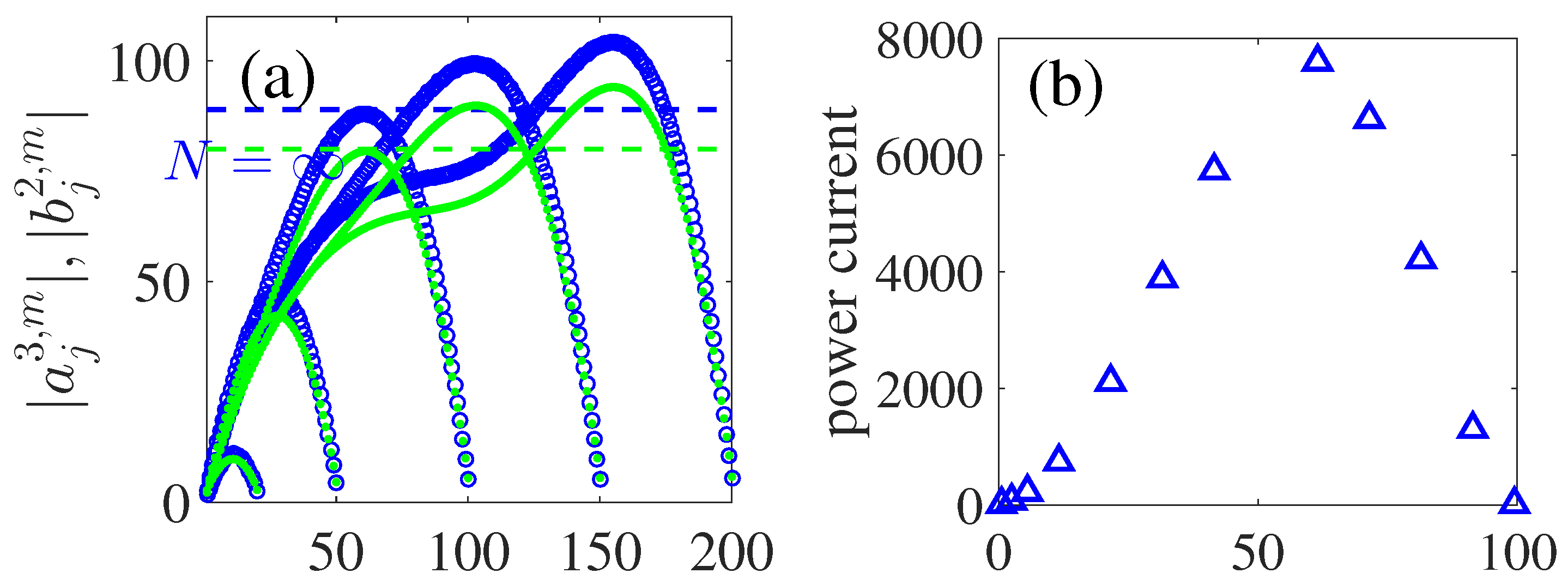
11. Array with the Finite Number of Dielectric Spheres

For finite number of the spheres the translational invariance is broken. Then Equation (2) can be modified as follows [24]

$$\begin{array}{c}\hfill \mathbf{E}\left(\mathbf{r}\right)=\sum _{j=1}^N\sum _{lm}[a_j^{lm}{\mathbf{M}}_l^m(\mathbf{r}-{\mathbf{R}}_j)+b_j^{lm}{\mathbf{N}}_l^m(\mathbf{r}-{\mathbf{R}}_j)],\\ \hfill \mathbf{H}\left(\mathbf{r}\right)=-i\sum _{j=1}^N\sum _{lm}[a_j^{lm}{\mathbf{N}}_l^m(\mathbf{r}-{\mathbf{R}}_j)+b_j^{lm}{\mathbf{M}}_l^m(\mathbf{r}-{\mathbf{R}}_j)].\end{array}$$

(61)

The expansion coefficients $a_j^{lm},b_j^{lm}$ were found numerically [11] and presented in Figure 27.

At the first sight it seems that for growing N the solution for amplitudes $a_j$ and $b_j$ should saturate except in the vicinity of the edges of the finite array. However the EM field is a massless field which has no characteristic scale. Hence we have the behavior of the amplitudes as shown in Figure 27. Nevertheless we can see a tendency for saturation of the amplitudes to the maximal value with the growth of N, but we always observe non-negligible effect of the edges of the finite array. That affects the transfer of SAM of incident light into the giant vortical currents in the vicinity of a quasi-BSC. A similar effect which transforms the BSCs into quasi-BSCs is the volatility of the material parameters of the spheres.

12. Summary and Discussion

Recently the BSCs above the light line were shown to exist in various systems of one-dimensional arrays of dielectric rods and holes in a dielectric slab [31,32,33,37,38,44,45,46]. Similar acoustic BSCs called embedded trapped Rayleigh-Bloch surface waves were obtained in system of material rods [26,29,47,98]. One could ask why BSCs occur in periodic dielectric structures (gratings) but not in homogeneous structures like a slab or a rod which can support guided EM modes below the light line only. Let us begin with the simplest textbook system of a dielectric slab infinitely long in the $x,y$ plane with the dielectric constant $ϵ>1$. The Maxwell equations can be solved by separation of variables for scalar function $\psi (x,y,z)=e^{i{k}_{x}x+i{k}_{y}y}\psi \left(z\right)$ to result in bound states below the light line $k_0^2=k_x^2+k_y^2$ [99] while all solutions above the light line are leaky [100]. The situation can be cardinally changed by replacing the continual translational symmetry by the discrete symmetry $ϵ(x,y,z)=ϵ(x+p,y,z)$ where $p=0,\pm 1,\pm 2,\dots$. All space variables are measured in the period length.. Then the radiation continua of plane waves $e^{i{k}_{x,n}x+i{k}_{y}y+i{k}_{z}z}$ are quantized $k_{x,n}=\beta +2\pi n,n=0,\pm 1,\pm 2,\dots$ with the frequency $k_0^2=k_{x,n}^2+k_y^2+k_z^2$. Here β is the Bloch wave vector along the x-axis, and the integer n refers to the diffraction continua [33]. The physical interpretation of this statement is related to that the slab with the discrete translational symmetry can be considered as a one-dimensional diffraction lattice in the x-direction. Let us take for simplicity $\beta =0,k_y=0$. Assume there is a bound solution with the eigenfrequency $k_{0,BSC}>0$ which is coupled with all diffraction continua enumerated by n. Let $k_{0,BSC}<2\pi$, i.e., the BSC resides in the first diffraction continua but below the others. Because of the symmetry or by variation of the material parameters of the modulated slab we can achieve that the coupling of the solution with the first diffraction continuum equals zero [37,38,44,45,46]. However the solution is coupled with evanescent continua $n=1,2,\dots$ giving rise to exponential decay of the bound solution over the z-axis. The length of localization is given by $L\sim \frac{1}{\sqrt{4{\pi }^2-k_{0,BSC}^2}}$. Therefore, the evanescent diffraction continua play a principal role in the space configuration of the BSCs. Moreover, one can see from Figure 5 that in the limit $h\to \infty$ the BSCs frequency $k_{0BSC}\to 0$ to leave no room for the BSCs with $k_{0,BSC}>0$.

In the present paper we chose another strategy to quantize the radiation continuum. We replace the rod with continual translational symmetry by a periodic array of dielectric spheres. Because of the axial symmetry of the array aligned along the z-axis the quantized continua are specified by two integers, m and n. The first integer is the azimuthal quantum number and the second number defines discrete directions of outgoing cylindrical waves (17) given by the wave vector $k_{z,n}=\beta +2\pi n$ in each sector m where β is the Bloch vector along the array. Bottoms of the particular continua with $m=0$ and $n=0,\pm 1$ and $n=-2$ are shown in Figure 5. By arguments similar to those presented above for the grated slab we obtain that the BSC with $\beta =0$ embedded into the first radiation continuum $m=0,n=0$ is localized around the array.

The symmetry of the system is also important for classifications of the BSCs which are labelled by the azimuthal number of the continuum m of cylindrical vectorial waves and the Bloch wave vector β. The symmetry properties of the BSC play a very important role since it is difficult to provide a zero coupling even with the lowest continua $n=0$ because of the degeneracy in polarization. Nevertheless the symmetry allows to decouple the BSC at least with some particular continua.

(1)

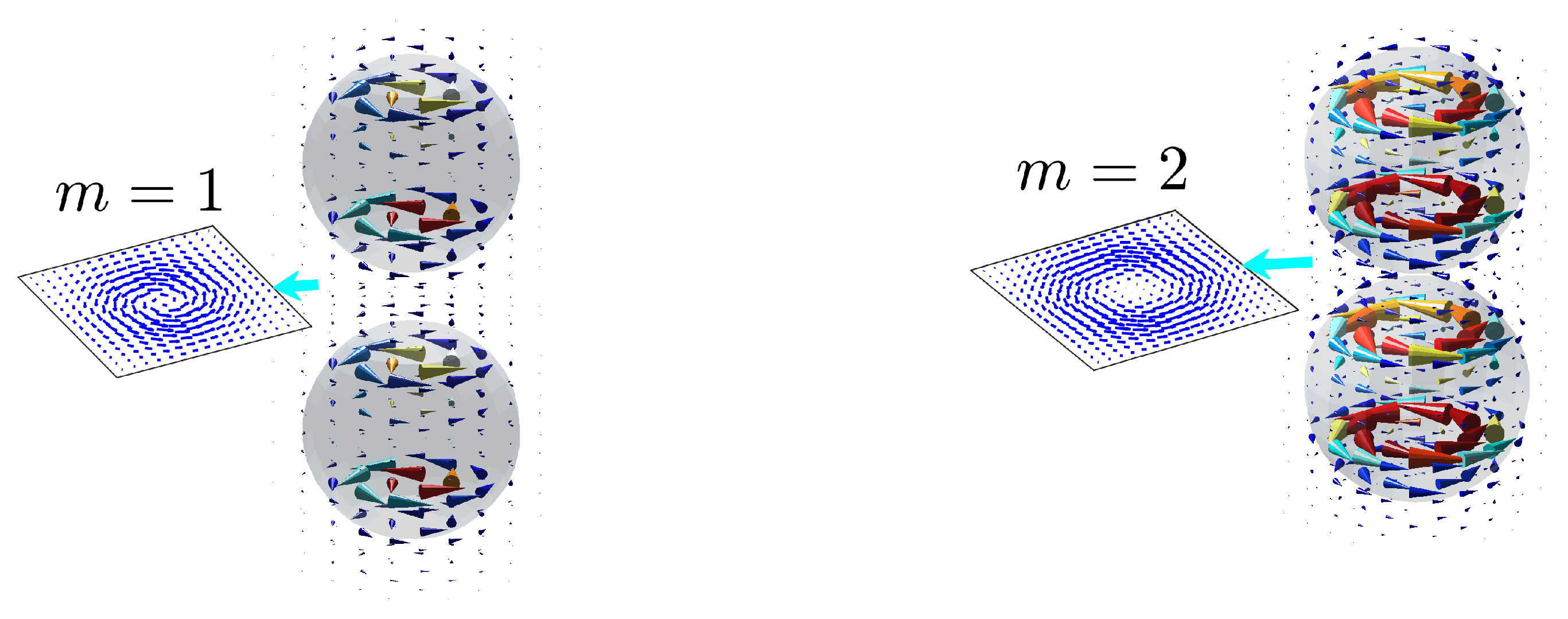
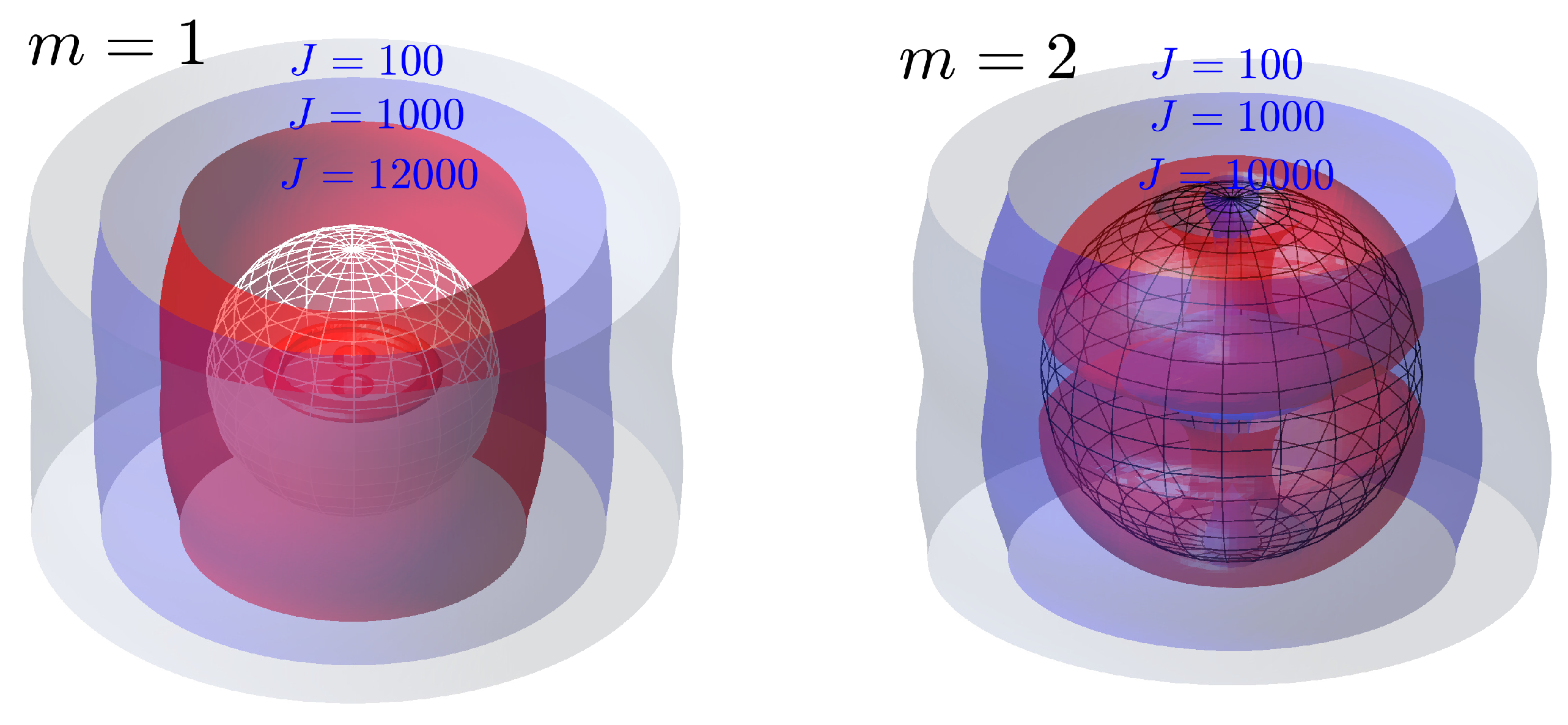
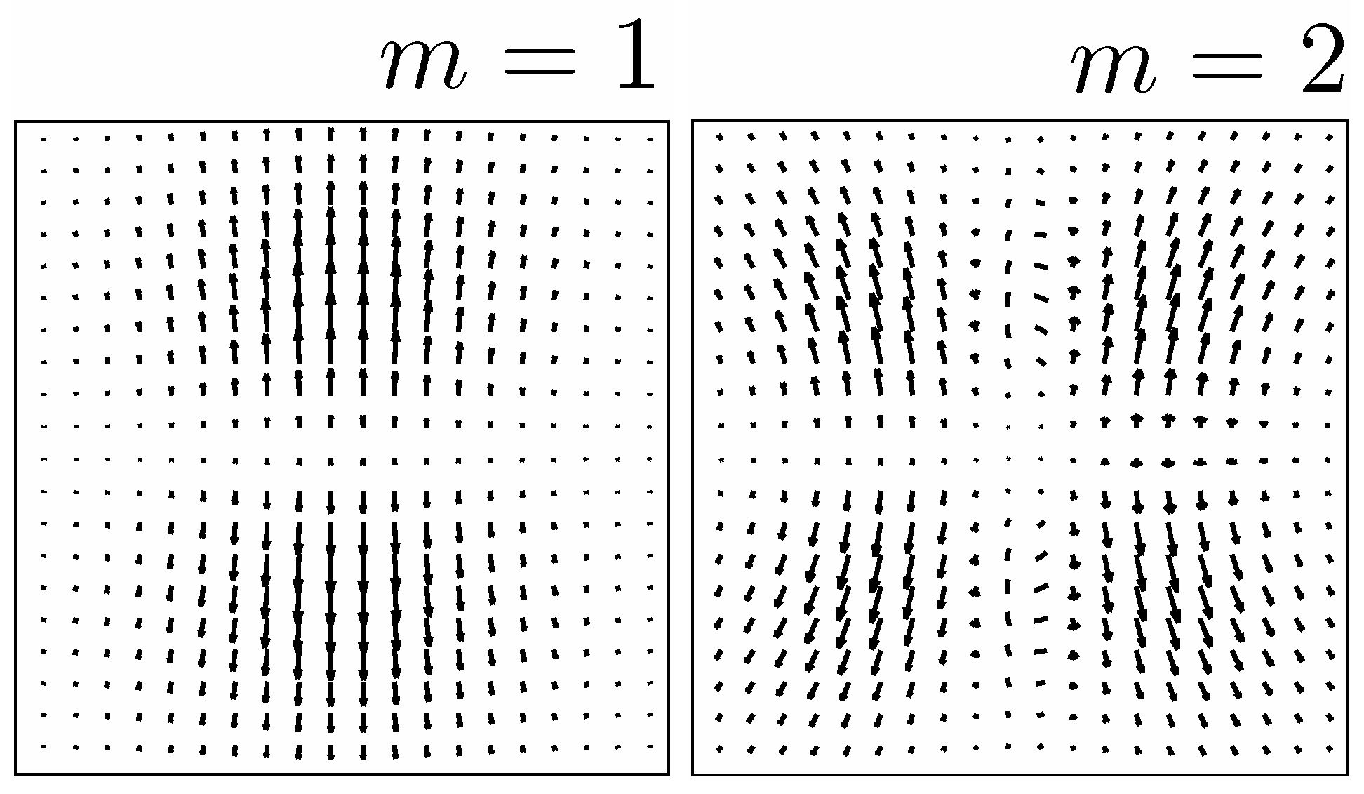
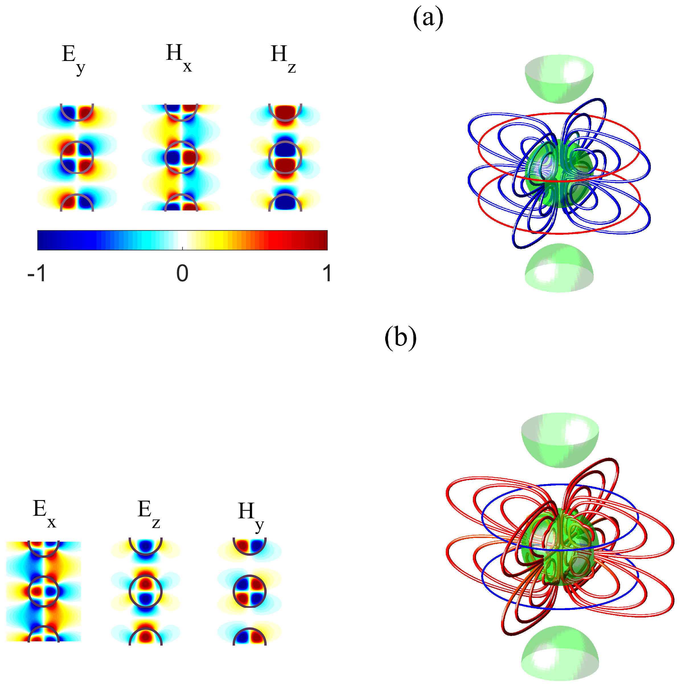
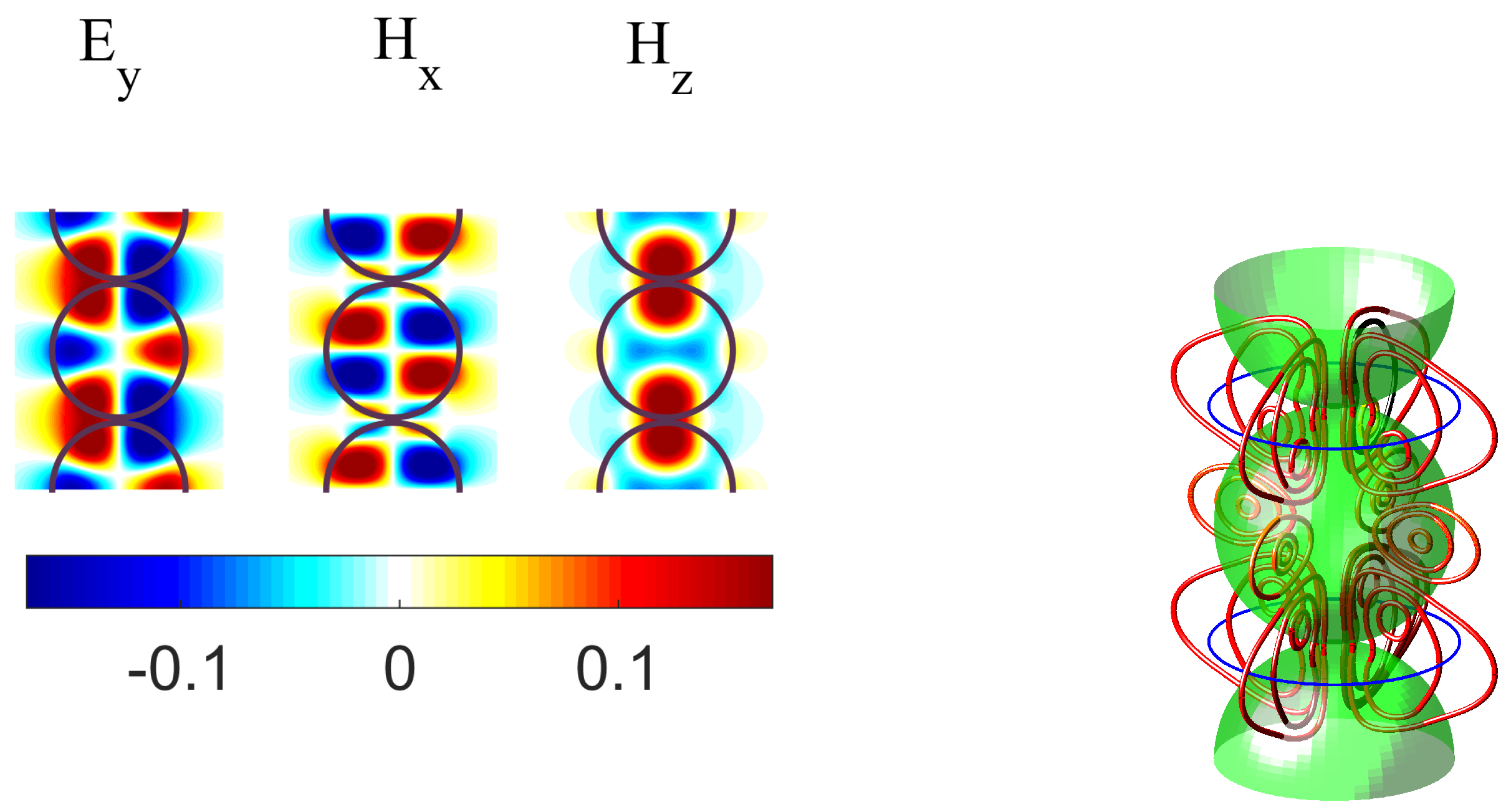
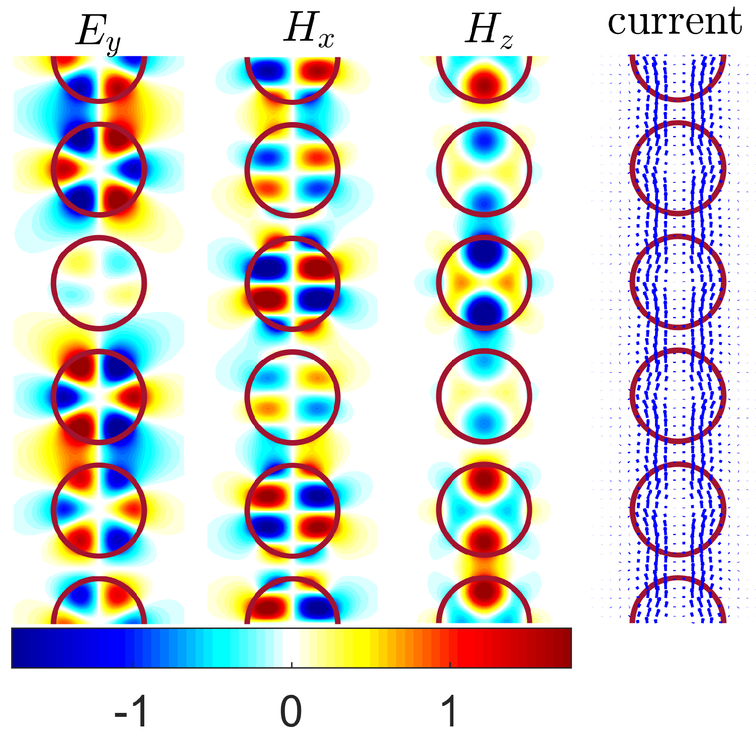
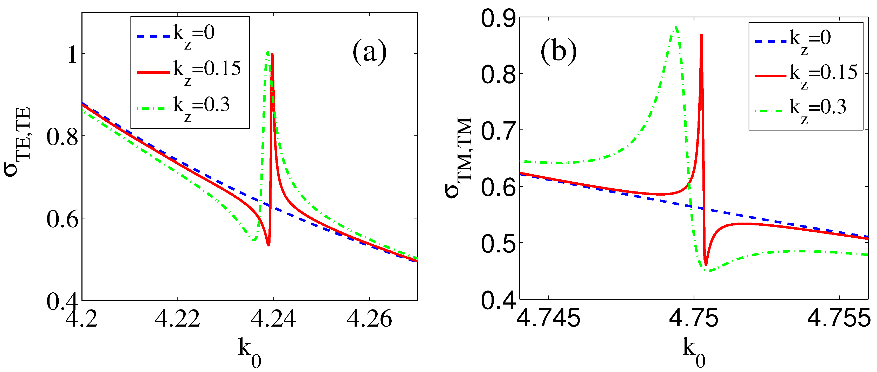
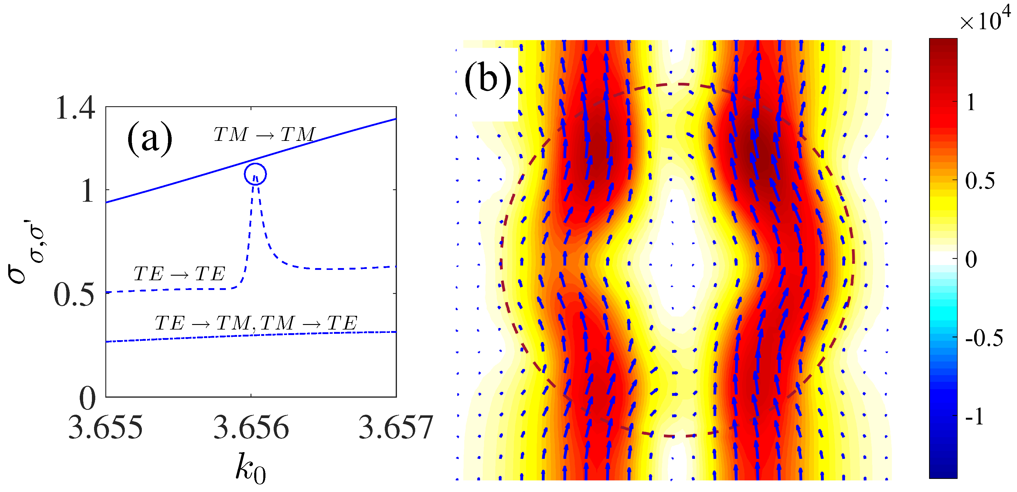
The symmetry protected BSCs constitute the vast majority of BSCs which are symmetrically mismatched with the first diffraction continuum $m=0,n=0$ of both polarizations. The EM field configurations of such BSCs presented in Figure 2 show hybridizations of a few orbital numbers $l=2,4,6,\dots$ which specify the BSCs as multipoles of high order. Therefore the BSC solutions can not be obtained by the use of the dipole approximation [20,21]. The most remarkable property from experimental viewpoint is the robustness of the BSCs relative to choice of the material parameters of the dielectric spheres. We present in Figure 3 an example of the BSC which is symmetry protected relative to the TM diffraction continuum but a zero coupling to the TE continuum obtained through variation of the sphere radius.

(2)

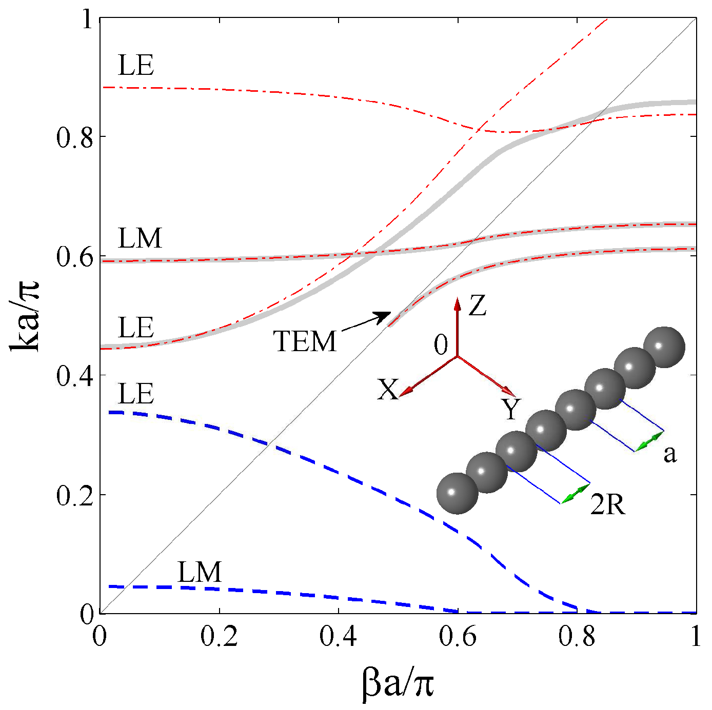
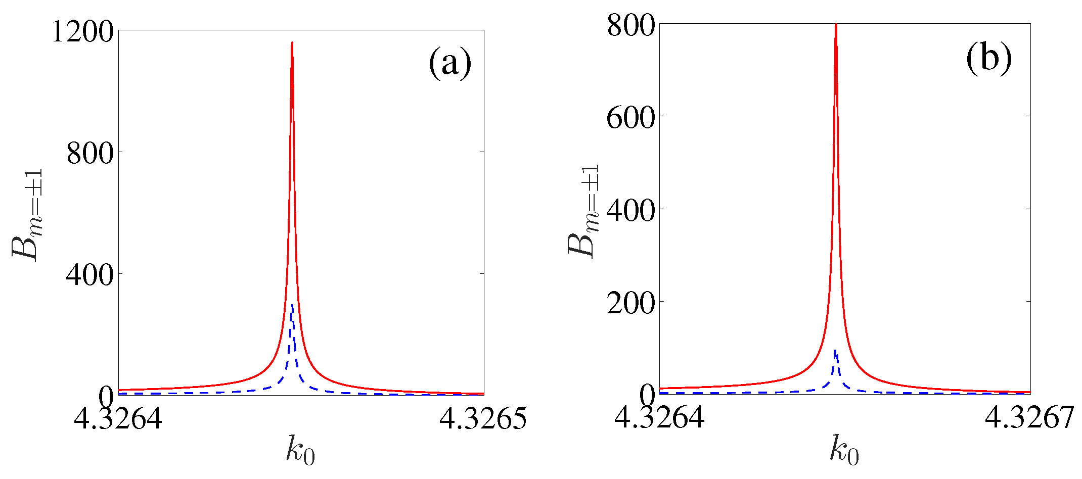
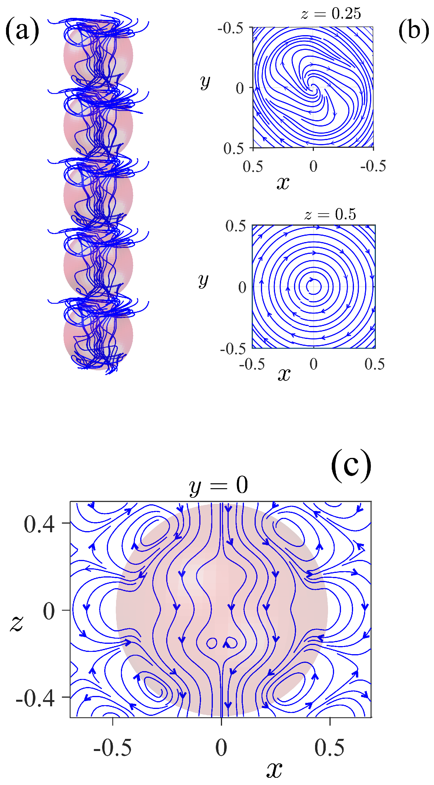
We demonstrated that the BSC can be accessed not only by variation of the material parameters but also by variation of Bloch wave vector β along the array axis. Patterns of the Bloch BSCs are presented in Figure 3.

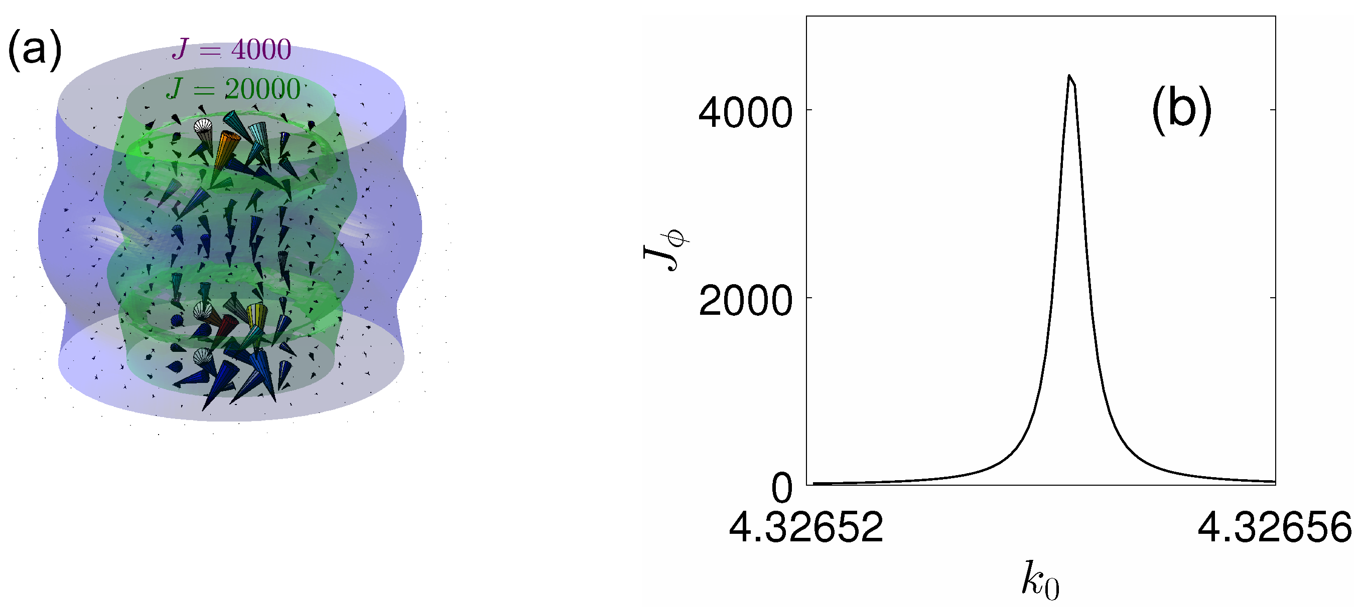
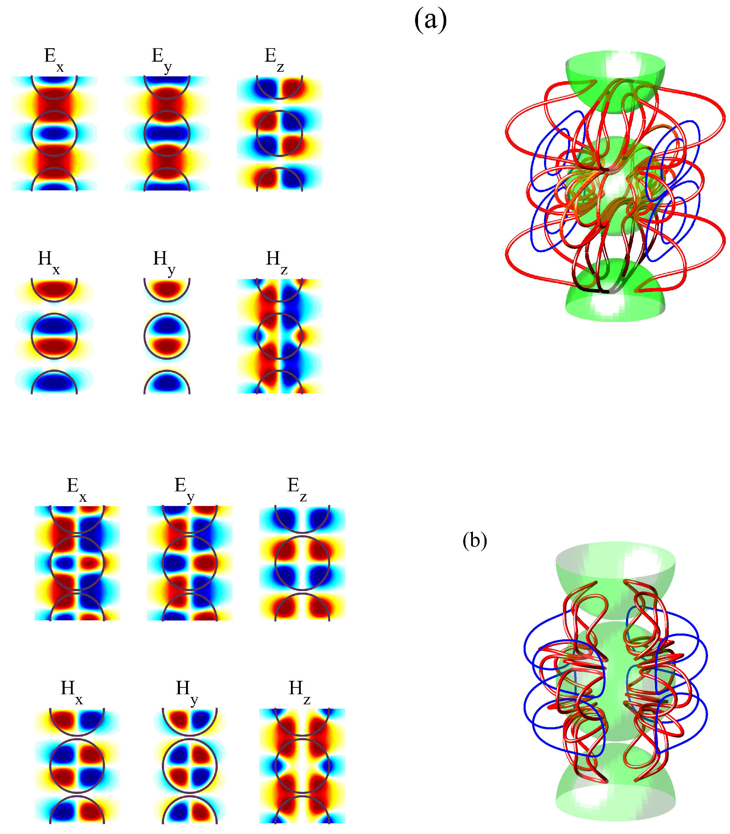
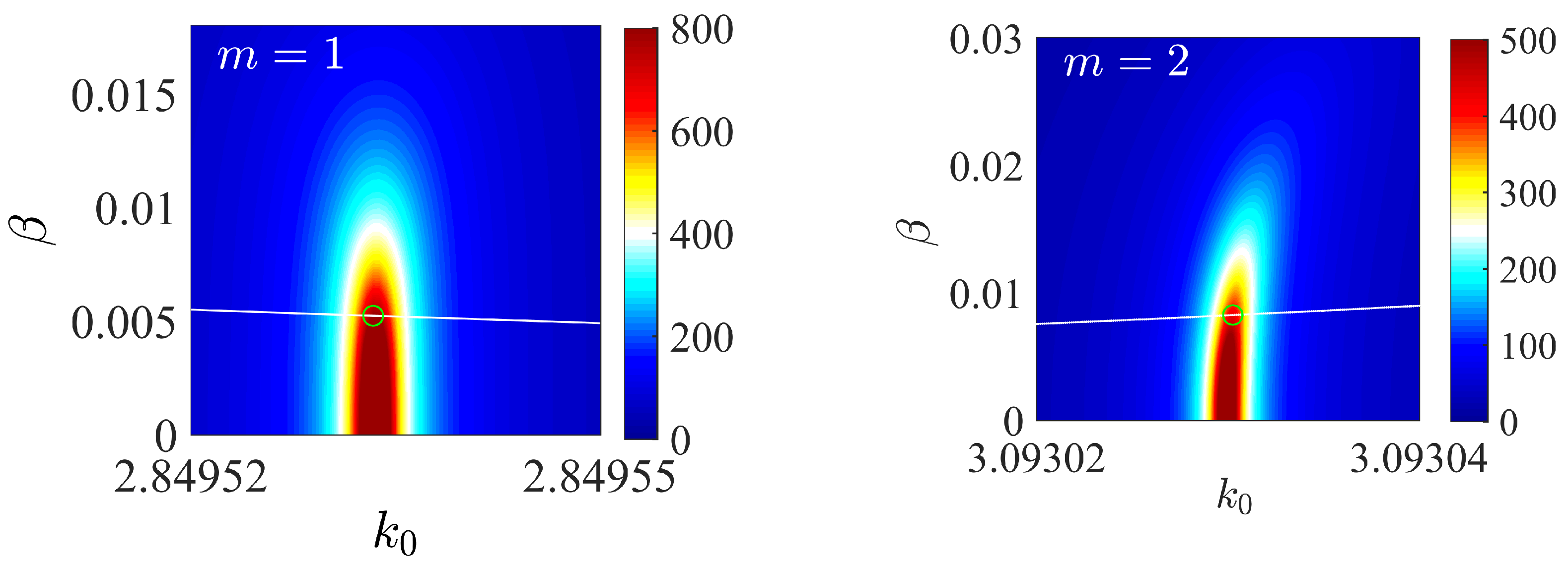
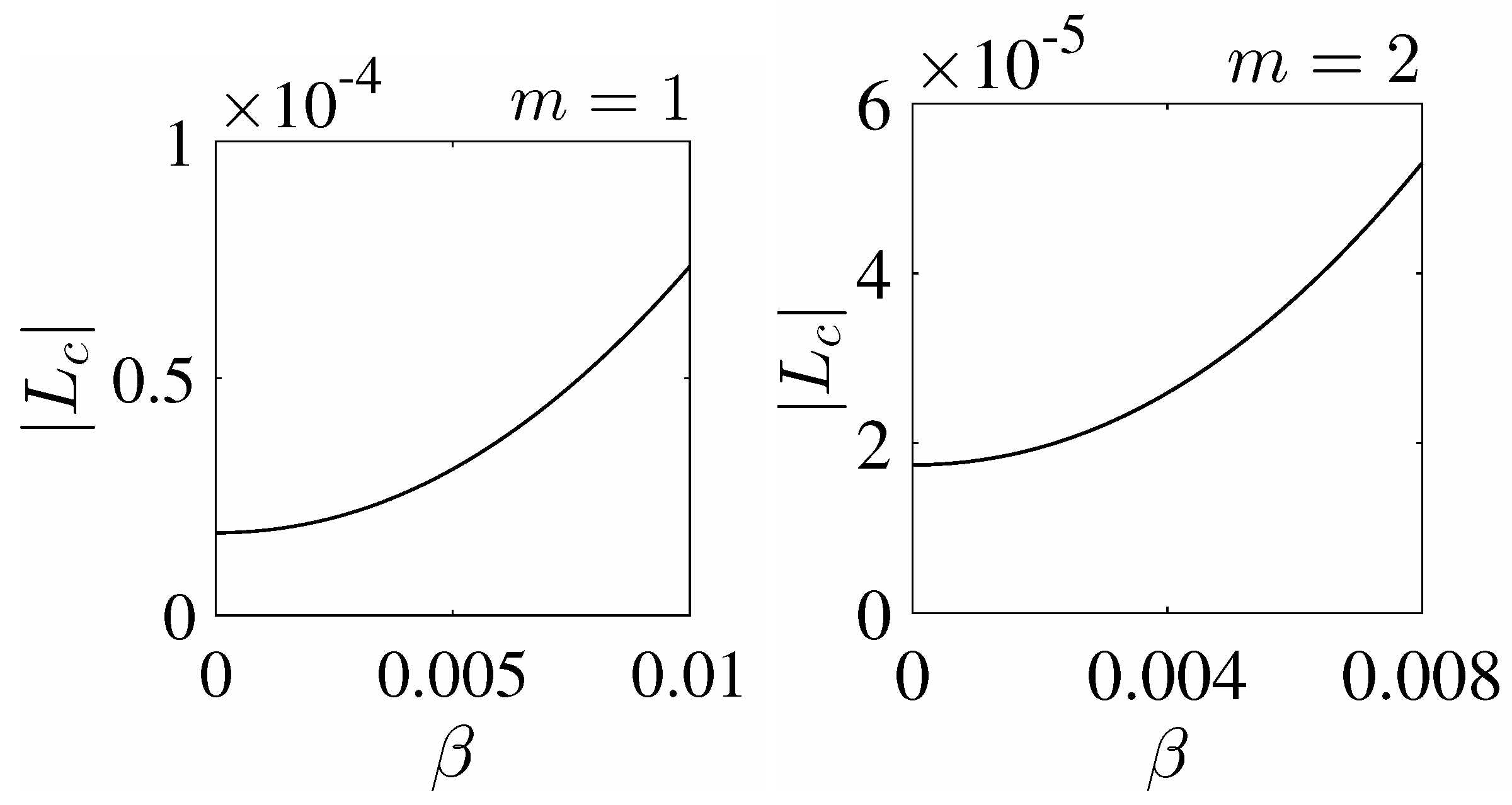
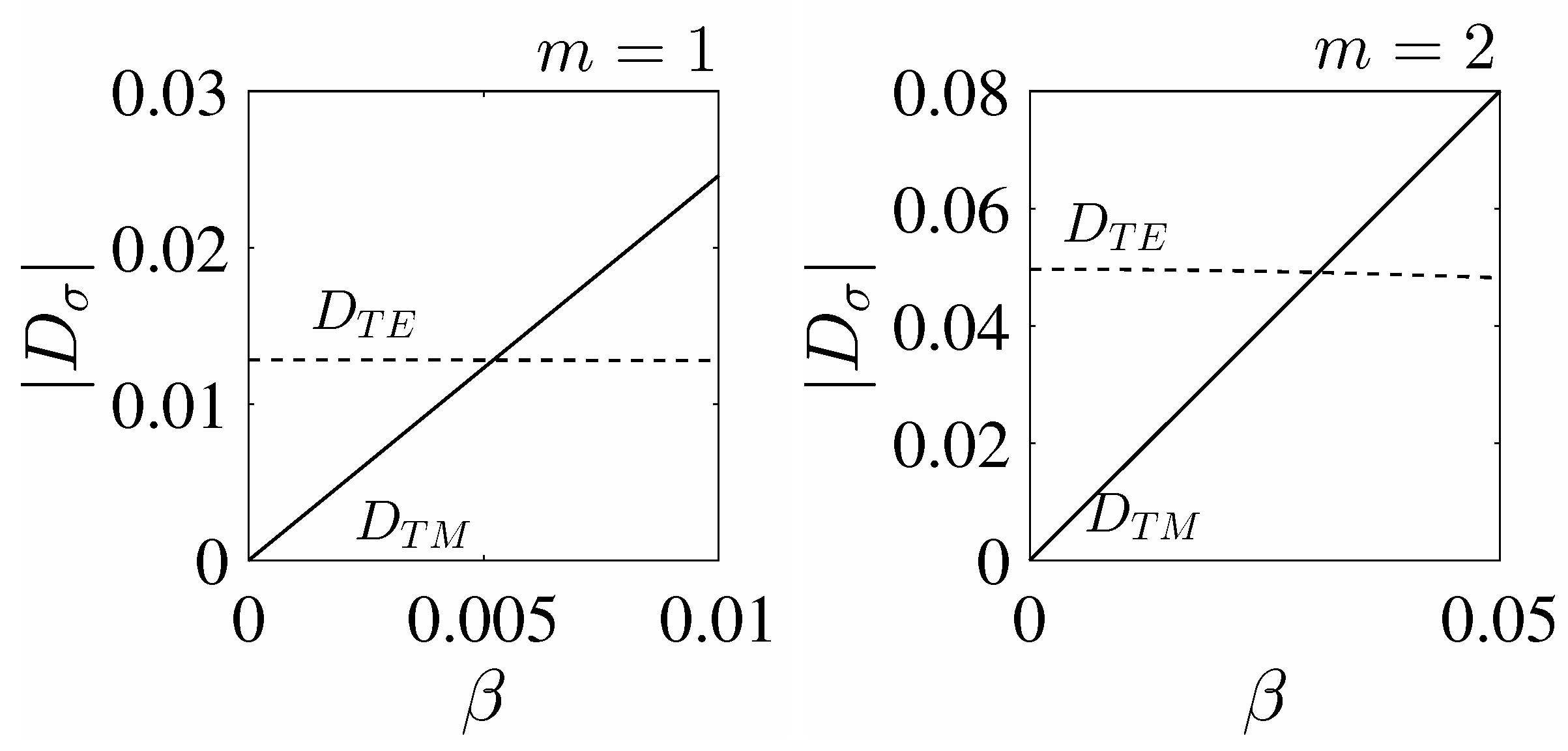
(3)

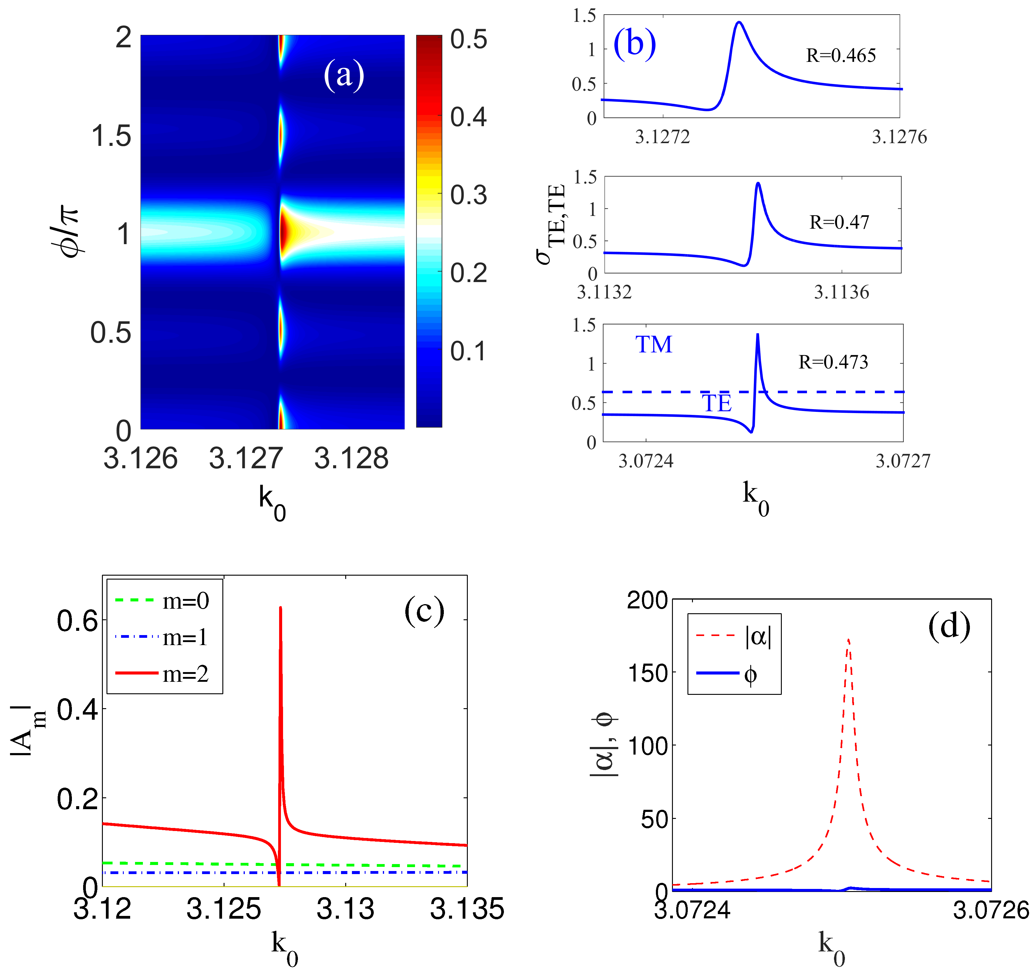
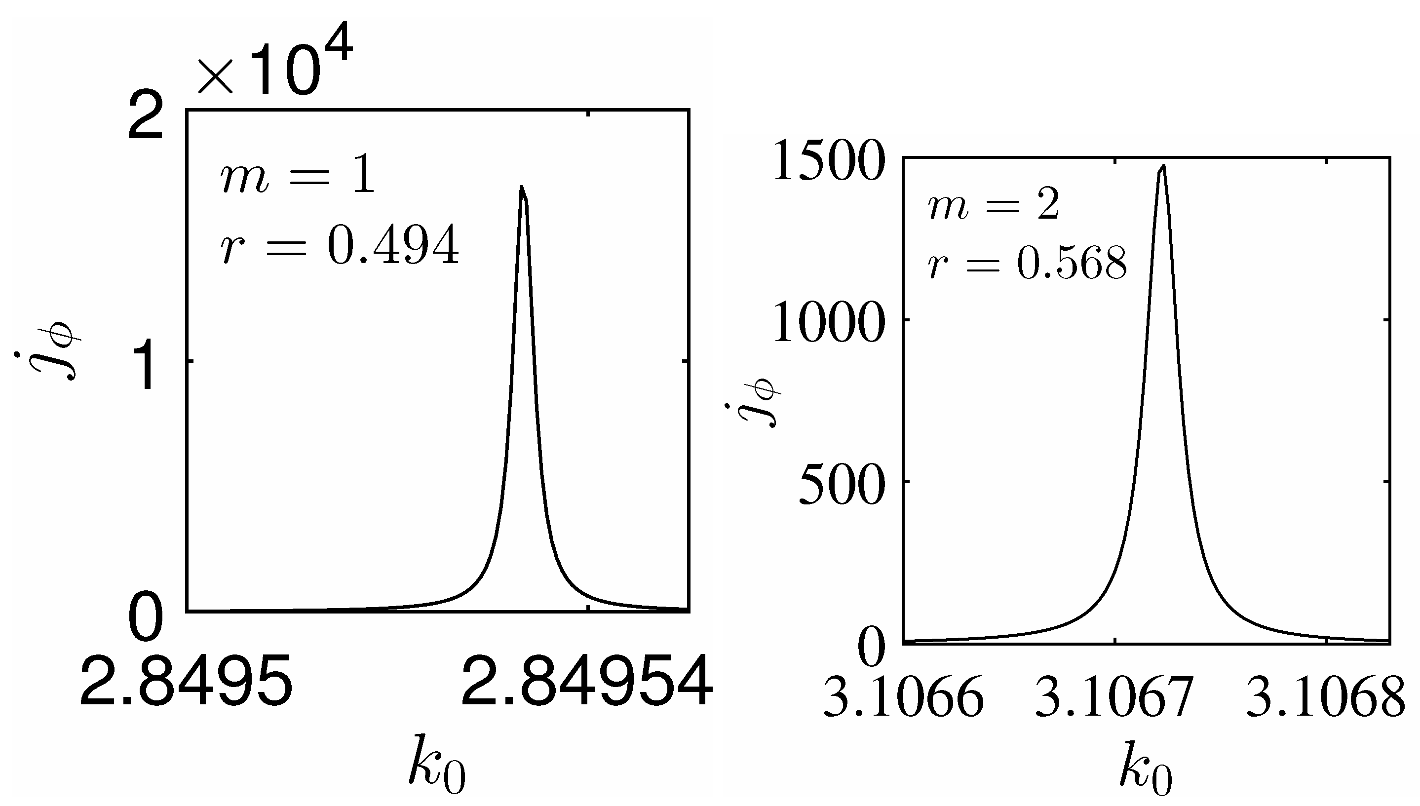
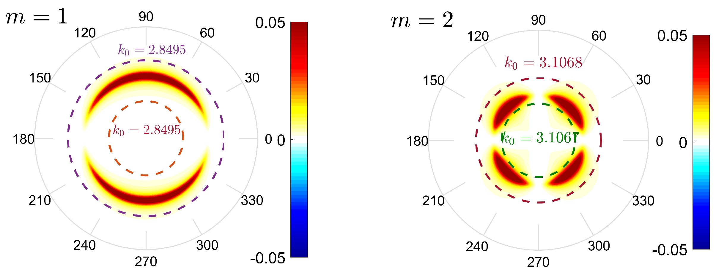
By tuning of the radius of the spheres we found BSCs in the next sectors of continua with $m\ne 0$. These BSCs shown in Figure 4 are remarkable by that they carry the OAM with spinning Poynting vectors.

(4)

The most sophisticated Bloch BSCs with OAM demonstrate spiralling Poynting vector as shown in Figure 24 and Figure 25.

The advantage of dielectric structures is a high quality factor and a wide range of BSC wavelengths from microns (photonics) to centimeter (microwave) as dependent on the choice of the radius of the spheres. Although the BSCs exist only in selected points in the parametric space there is a nearest vicinity of the BSC point where the BSC predominantly contributes into the cross-section and the EM field in the near field zone as seen from Figure 10 and Figure 11. That leads to extremely efficient light harvesting capabilities [83]. The far zone EM fields can also show abundant features related to the BSCs. In particular Figure 11a demonstrates the effect of antenna when the BSC with azimuthal number $m=2$ converts the EM energy into the perpendicular directions.

The BSCs with OAM $m=\pm 1$ emerge in the response of the array to incident plane waves with circular polarization. A transfer of the SAM of the incident plane wave into the OAM of EM field takes place for any frequency and wave vector of the incident wave as shown in Figure 13. The transfer results in the power current spinning around the array. The most remarkable is that as seen from Figure 13 and Figure 16 in the nearest vicinity of the BSCs with $m\ne 0$ the array supports giant vortical power currents which are directly related to the extremal enhancement of the scattered field. The value of the current is also sensitive to the distance from the array. It rapidly goes down away from spheres as shown in Figure 19.

Theoretically the value of the circulating currents can grow up to infinity in the BSC point. However there is a difference between the present theory and possible experimental realization of the transfer of SAM into OAM, that is (1) a finite number of the spheres and (2) there are always some losses when the waves transport through the sample because of material for spheres. The most profound effect of finite arrays is that the BSCs become quasi-BSCs because, unlike a plasmonic sphere, finite dielectric systems can not support BSCs [101,102,103]. Therefore the effect of giant vortical currents around the array can be suppressed. Indeed, as our calculations show in Figure 27 for finite number N the currents decay for approaching to ends of the array. However with since $N\ge 100$ at middle of the array the BSC is restoring.

The next problem which can seriously damage the effect of giant spinning currents is the complex dielectric permittivity $ϵ={ϵ}^{\prime }+i{ϵ}^{″}$. Fortunately, for silicon dielectric particles there is a wide frequency window in the nearest infrared range where the ${ϵ}^{″}$ is extremely small [75]. The advantage of dielectric structures is a wide range of BSC wavelengths from microns (photonics) to centimeter (microwave range) as dependent on the choice of the radius of spheres. Losses when the waves transport through the array result in the finite free path length $L=v_g/{ϵ}^{″}\omega$ where $v_g$ is the group velocity. Therefore it is sufficient to take the number of spheres not exceeding $L/h$ where h is the period of the array. This problem was considered in details in Ref. [57].

Moreover we have shown the propagating Bloch BSC with both $\beta \ne 0$ and OAM $m=\pm 1$ for the array of dielectric particles with the permittivity around 10. The Bloch vector ${\beta }_c$ can be tuned by variation of the permittivity. Although we revealed only the value of OAM $m=\pm 1$ in general there is no restriction for the Bloch BSCs with OAM $\left|m\right|>1$. To the best of our knowledge, the BSCs with OAM guided along the array has not been previously advanced as a possible fundamental effect for device applications. One of the most important application we consider that the array is capable for lasing through the BSC as it was demonstrated in Refs. [104,105]. However the principal feature of lasing by the array of dielectric spheres is that the laser beam carries the OAM without use of special chiral symmetry broken media [86,90,91].

References

1. Stratton, J.A. Electromagnetic Theory; McGraw-Hill Book Company, Inc.: NewYork, NY, USA, 1941. [Google Scholar]
2. Ohtaka, K. Energy band of photons and low-energy photon diffraction. Phys. Rev. B 1979, 19, 5057–5067. [Google Scholar] [CrossRef]
3. Ohtaka, K. Scattering theory of low-energy photon diffraction. J. Phys. C Solid State Phys. 1980, 13, 667–680. [Google Scholar] [CrossRef]
4. Miyazaki, H.; Ohtaka, K. Near-field images of a monolayer of periodically arrayed dielectric spheres. Phys. Rev. B 1998, 58, 6920–6937. [Google Scholar] [CrossRef]
5. Modinos, A. Scattering of electromagnetic waves by a plane of spheres-formalism. Phys. A Stat. Mech. Its Appl. 1987, 141, 575–588. [Google Scholar] [CrossRef]
6. Bruning, J.; Lo, Y. Multiple scattering of EM waves by spheres part I—Multipole expansion and ray-optical solutions. IEEE Trans. Antennas Propag. 1971, 19, 378–390. [Google Scholar] [CrossRef]
7. García de Abajo, F.J. Colloquium: Light scattering by particle and hole arrays. Rev. Mod. Phys. 2007, 79, 1267–1290. [Google Scholar] [CrossRef]
8. Wang, K.X.; Yu, Z.; Sandhu, S.; Liu, V.; Fan, S. Condition for perfect antireflection by optical resonance at material interface. Optica 2014, 1, 388. [Google Scholar] [CrossRef]
9. Fuller, K.A.; Kattawar, G.W. Consummate solution to the problem of classical electromagnetic scattering by an ensemble of spheres I: Linear chains. Opt. Lett. 1988, 13, 90–92. [Google Scholar] [CrossRef] [PubMed]
10. Hamid, A.K.; Ciric, I.; Hamid, M. Iterative solution of the scattering by an arbitrary configuration of conducting or dielectric spheres. IEE Proc. H Microw. Antennas Propag. 1991, 138, 565. [Google Scholar] [CrossRef]
11. Xu, Y.L. Electromagnetic scattering by an aggregate of spheres. Appl. Opt. 1995, 34, 4573–4588. [Google Scholar] [CrossRef] [PubMed]
12. Mackowski, D.W. Calculation of total cross sections of multiple-sphere clusters. J. Opt. Soc. Am. A 1994, 11, 2851–2861. [Google Scholar] [CrossRef]
13. Quirantes, A.; Arroyo, F.; Quirantes-Ros, J. Multiple light scattering by spherical particle systems and its dependence on concentration: A T-matrix study. J. Colloid Interface Sci. 2001, 240, 7882. [Google Scholar] [CrossRef] [PubMed]
14. Luan, P.G.; Chang, K.D. Transmission characteristics of finite periodic dielectric waveguides. Opt. Express 2006, 14, 3263–3272. [Google Scholar] [CrossRef] [PubMed]
15. Zhao, R.; Zhai, T.; Wang, Z.; Liu, D. Guided resonances in periodic dielectric waveguides. J. Lightwave Technol. 2009, 27, 4544–4547. [Google Scholar] [CrossRef]
16. Du, J.; Liu, S.; Lin, Z.; Zi, J.; Chui, S.T. Guiding electromagnetic energy below the diffraction limit with dielectric particle arrays. Phys. Rev. A 2009, 79, 205436. [Google Scholar] [CrossRef]
17. Burin, A.L.; Cao, H.; Schatz, G.C.; Ratner, M.A. High-quality optical modes in low-dimensional arrays of nanoparticles: Application to random lasers. J. Opt. Soc. Am. B 2004, 21, 121–131. [Google Scholar] [CrossRef]
18. Gozman, M.; Polishchuk, I.; Burin, A. Light propagation in linear arrays of spherical particles. Phys. Lett. A 2008, 372, 5250–5253. [Google Scholar] [CrossRef]
19. Blaustein, G.S.; Gozman, M.I.; Samoylova, O.; Polishchuk, I.Y.; Burin, A.L. Guiding optical modes in chains of dielectric particles. Opt. Express 2007, 15, 17380–17391. [Google Scholar] [CrossRef] [PubMed]
20. Draine, B.T.; Flatau, P.J. Discrete-dipole approximation for periodic targets: Theory and tests. J. Opt. Soc. Am. A 2008, 25, 2693–2703. [Google Scholar] [CrossRef]
21. Savelev, R.S.; Slobozhanyuk, A.P.; Miroshnichenko, A.E.; Kivshar, Y.S.; Belov, P.A. Subwavelength waveguides composed of dielectric nanoparticles. Phys. Rev. B 2014, 89, 035435. [Google Scholar] [CrossRef]
22. Savelev, R.S.; Filonov, D.S.; Petrov, M.I.; Krasnok, A.E.; Belov, P.A.; Kivshar, Y.S. Resonant transmission of light in chains of high-index dielectric particles. Phys. Rev. B 2015, 92, 155415. [Google Scholar] [CrossRef]
23. Li, S.V.; Baranov, D.G.; Krasnok, A.E.; Belov, P.A. All-dielectric nanoantennas for unidirectional excitation of electromagnetic guided modes. Appl. Phys. Lett. 2015, 107, 171101. [Google Scholar] [CrossRef]
24. Linton, C.; Zalipaev, V.; Thompson, I. Electromagnetic guided waves on linear arrays of spheres. Wave Motion 2013, 50, 29–40. [Google Scholar] [CrossRef] [Green Version]
25. Bonnet-Bendhia, A.S.; Starling, F. Guided waves by electromagnetic gratings and non-uniqueness examples for the diffraction problem. Math. Methods Appl. Sci. 1994, 17, 305–338. [Google Scholar] [CrossRef]
26. Porter, R.; Evans, D.V. Rayleigh-Bloch surface waves along periodic gratings and their connection with trapped modes in waveguides. J. Fluid Mech. 1999, 386, 233–258. [Google Scholar] [CrossRef]
27. Evans, D.V.; Porter, R. Trapping and near-trapping by arrays of cylinders in waves. J. Eng. Math. 1999, 35, 149179. [Google Scholar] [CrossRef]
28. Cohen, O.; Freedman, B.; Fleischer, J.W.; Segev, M.; Christodoulides, D.N. Grating-mediated waveguiding. Phys. Rev. Lett. 2004, 93, 103902. [Google Scholar] [CrossRef] [PubMed]
29. Porter, R.; Evans, D. Embedded Rayleigh-Bloch surface waves along periodic rectangular arrays. Wave Motion 2005, 43, 29–50. [Google Scholar] [CrossRef]
30. Venakides, S.; Shipman, S.P. Resonance and bound states in photonic crystal slabs. SIAM J. Appl. Math. 2003, 64, 322–342. [Google Scholar] [CrossRef]
31. Shipman, S.P.; Venakides, S. Resonant transmission near nonrobust periodic slab modes. Phys. Rev. E 2005, 71, 026611. [Google Scholar] [CrossRef] [PubMed]
32. Marinica, D.C.; Borisov, A.G.; Shabanov, S.V. Bound states in the continuum in photonics. Phys. Rev. Lett. 2008, 100, 183902. [Google Scholar] [CrossRef] [PubMed]
33. Ndangali, R.F.; Shabanov, S.V. Electromagnetic bound states in the radiation continuum for periodic double arrays of subwavelength dielectric cylinders. J. Math. Phys. 2010, 51, 102901. [Google Scholar] [CrossRef]
34. Hsueh, W.; Chen, C.; Chang, C. Bound states in the continuum in quasiperiodic systems. Phys. Lett. A 2010, 374, 4804–4807. [Google Scholar] [CrossRef]
35. Hsu, C.W.; Zhen, B.; Lee, J.; Chua, S.L.; Johnson, S.G.; Joannopoulos, J.D.; Soljačić, M. Observation of trapped light within the radiation continuum. Nature 2013, 499, 188–191. [Google Scholar]
36. Weimann, S.; Xu, Y.; Keil, R.; Miroshnichenko, A.E.; Tünnermann, A.; Nolte, S.; Sukhorukov, A.A.; Szameit, A.; Kivshar, Y.S. Compact Surface Fano States Embedded in the Continuum of Waveguide Arrays. Phys. Rev. Lett. 2013, 111, 240403. [Google Scholar] [CrossRef] [PubMed]
37. Bulgakov, E.N.; Sadreev, A.F. Bloch bound states in the radiation continuum in a periodic array of dielectric rods. Phys. Rev. A 2014, 90, 053801. [Google Scholar] [CrossRef]
38. Hu, Z.; Lu, Y.Y. Standing waves on two-dimensional periodic dielectric waveguides. J. Opt. 2015, 17, 065601. [Google Scholar] [CrossRef]
39. Bykov, D.A.; Doskolovich, L.L. ωkx Fano line shape in photonic crystal slabs. Phys. Rev. A 2015, 92, 013845. [Google Scholar] [CrossRef]
40. Song, M.; Yu, H.; Wang, C.; Yao, N.; Pu, M.; Luo, J.; Zhang, Z.; Luo, X. Sharp Fano resonance induced by a single layer of nanorods with perturbed periodicity. Opt. Express 2015, 23, 2895–2903. [Google Scholar] [CrossRef] [PubMed]
41. Zou, C.L.; Cui, J.M.; Sun, F.W.; Xiong, X.; Zou, X.B.; Han, Z.F.; Guo, G.C. Guiding light through optical bound states in the continuum for ultrahigh-Qmicroresonators. Laser Photonics Rev. 2014, 9, 114–119. [Google Scholar] [CrossRef]
42. Wang, Z.; Zhang, H.; Ni, L.; Hu, W.; Peng, C. Analytical Perspective of Interfering Resonances in High-Index-Contrast Periodic Photonic Structures. IEEE J. Quantum Electron. 2016, 52, 6100109. [Google Scholar] [CrossRef]
43. Li, L.; Yin, H. Bound States in the Continuum in double layer structures. Sci. Rep. 2016, 6, 26988. [Google Scholar] [CrossRef] [PubMed]
44. Hsu, C.W.; Zhen, B.; Chua, S.L.; Johnson, S.G.; Joannopoulos, J.D.; Soljačić, M. Bloch surface eigenstates within the radiation continuum. Light Sci. Appl. 2013, 2, e84. [Google Scholar] [CrossRef]
45. Zhen, B.; Hsu, C.W.; Lu, L.; Stone, A.D.; Soljačić, M. Topological Nature of Optical Bound States in the Continuum. Phys. Rev. Lett. 2014, 113, 257401. [Google Scholar] [CrossRef] [PubMed]
46. Yang, Y.; Peng, C.; Liang, Y.; Li, Z.; Noda, S. Analytical Perspective for Bound States in the Continuum in Photonic Crystal Slabs. Phys. Rev. Lett. 2014, 113, 037401. [Google Scholar] [CrossRef] [PubMed]
47. Colquitt, D.J.; Craster, R.V.; Antonakakis, T.; Guenneau, S. Rayleigh-Bloch waves along elastic diffraction gratings. Proc. R. Soc. A Math. Phys. Eng. Sci. 2014, 471, 20140465. [Google Scholar] [CrossRef] [PubMed]
48. Gao, X.; Hsu, C.W.; Zhen, B.; Lin, X.; Joannopoulos, J.D.; Soljačić, M.; Chen, H. Formation Mechanism of Guided Resonances and Bound States in the Continuum in Photonic Crystal Slabs. arXiv, 2016; arXiv:1603.02815. [Google Scholar]
49. Hung, Y.J.; Lin, I.S. Visualization of Bloch surface waves and directional propagation effects on one-dimensional photonic crystal substrate. Opt. Express 2016, 24, 16003–16009. [Google Scholar] [CrossRef] [PubMed]
50. Blanchard, C.; Hugonin, J.P.; Sauvan, C. Fano resonances in photonic crystal slabs near optical bound states in the continuum. Phys. Rev. B 2016, 94, 155303. [Google Scholar] [CrossRef]
51. Wang, Y.; Song, J.; Dong, L.; Lu, M. Optical bound states in slotted high-contrast gratings. J. Opt. Soc. Am. B 2016, 33, 2472–2479. [Google Scholar] [CrossRef]
52. Zhang, M.; Zhang, X. Ultrasensitive optical absorption in graphene based on bound states in the continuum. Sci. Rep. 2015, 5, 8266. [Google Scholar] [CrossRef] [PubMed]
53. Padgett, M.; Courtial, J.; Allen, L. Light’s Orbital Angular Momentum. Phys. Today 2004, 57, 2004. [Google Scholar] [CrossRef]
54. Allen, L.; Padgett, M. The Poynting vector in Laguerre-Gaussian beams and the interpretation of their angular momentum density. Opt. Commun. 2000, 184, 67–71. [Google Scholar] [CrossRef]
55. Yao, A.M.; Padgett, M.J. Orbital angular momentum: Origins, behavior and applications. Adv. Opt. Photon. 2011, 3, 161. [Google Scholar] [CrossRef]
56. Bulgakov, E.N.; Sadreev, A.F. Light trapping above the light cone in a one-dimensional array of dielectric spheres. Phys. Rev. A 2015, 92, 023816. [Google Scholar] [CrossRef]
57. Bulgakov, E.; Maksimov, D.N. Light guiding above the light line in arrays of dielectric nanospheres. Opt. Lett. 2016, 41, 3888–3891. [Google Scholar] [CrossRef] [PubMed]
58. Bulgakov, E.N.; Sadreev, A.F. Transfer of spin angular momentum of an incident wave into orbital angular momentum of the bound states in the continuum in an array of dielectric spheres. Phys. Rev. A 2016, 94, 033856. [Google Scholar] [CrossRef]
59. Bulgakov, E.N.; Sadreev, A.F. Propagating Bloch waves with orbital angular momentum above the light cone in the array of dielectric spheres. J. Opt. Soc. Am. A 2017. submitted. [Google Scholar]
60. Hsu, C.W.; Zhen, B.; Stone, A.D.; Joannopoulos, J.D.; Soljačić, M. Bound states in the continuum. Nat. Rev. Mater. 2016, 1, 16048. [Google Scholar] [CrossRef]
61. Bykov, D.A.; Doskolovich, L.L. Numerical methods for calculating poles of the scattering matrix with applications in grating theory. J. Lightwave Technol. 2013, 31, 793–801. [Google Scholar] [CrossRef]
62. Yuan, L.J.; Lu, Y.Y. Propagating Bloch modes above the light line on a periodic array of cylinders. J. Phys. B 2016. [Google Scholar] [CrossRef]
63. Merchiers, O.; Moreno, F.; González, F.; Saiz, J.M. Light scattering by an ensemble of interacting dipolar particles with both electric and magnetic polarizabilities. Phys. Rev. A 2007, 76, 043834. [Google Scholar] [CrossRef]
64. Evlyukhin, A.B.; Reinhardt, C.; Seidel, A.; Luk’yanchuk, B.S.; Chichkov, B.N. Optical response features of Si-nanoparticle arrays. Phys. Rev. B 2010, 82, 045404. [Google Scholar] [CrossRef]
65. Wheeler, M.S.; Aitchison, J.S.; Mojahedi, M. Coupled magnetic dipole resonances in sub-wavelength dielectric particle clusters. J. Opt. Soc. Am. B 2010, 27, 1083–1091. [Google Scholar] [CrossRef]
66. Shore, R.A.; Yaghjian, A.D. Traveling Electromagnetic Waves on Linear Periodic Arrays of Small Lossless Penetrable Spheres; Technical Report, DTIC Document; Defense Technical Information Center: Fort Belvoir, VA, USA, 2004. [Google Scholar]
67. Shore, R.A.; Yaghjian, A.D. Travelling electromagnetic waves on linear periodic arrays of lossless spheres. Electron. Lett. 2005, 41, 578–580. [Google Scholar] [CrossRef]
68. Shore, R.A.; Yaghjian, A.D. Complex waves on periodic arrays of lossy and lossless permeable spheres: 1. Theory. Radio Sci. 2012, 47, RS2014. [Google Scholar] [CrossRef]
69. Deych, L.; Roslyak, A. Long-living collective optical excitations in a linear chain of microspheres. Phys. Status Solidi C 2005, 2, 3908–3911. [Google Scholar] [CrossRef]
70. Deych, L.I.; Roslyak, O. Photonic band mixing in linear chains of optically coupled microspheres. Phys. Rev. E 2006, 73, 036606. [Google Scholar] [CrossRef] [PubMed]
71. Monticone, F.; Alù, A. Embedded Photonic Eigenvalues in 3D Nanostructures. Phys. Rev. Lett. 2014, 112, 213903. [Google Scholar] [CrossRef]
72. Tikhodeev, S.G.; Yablonskii, A.L.; Muljarov, E.A.; Gippius, N.A.; Ishihara, T. Quasiguided modes and optical properties of photonic crystal slabs. Phys. Rev. B 2002, 66, 045102. [Google Scholar] [CrossRef]
73. Shore, R.A.; Yaghjian, A.D. Complex waves on periodic arrays of lossy and lossless permeable spheres: 2. Numerical results. Radio Sci. 2012, 47, RS2015. [Google Scholar] [CrossRef]
74. Carrasco, S.; Saleh, B.E.A.; Teich, M.C.; Fourkas, J.T. Second- and third-harmonic generation with vector Gaussian beams. J. Opt. Soc. Am. B 2006, 23, 2134–2141. [Google Scholar] [CrossRef]
75. Vuye, G.; Fisson, S.; Nguyen Van, V.; Wang, Y.; Rivory, J.; Abelès, F. Temperature dependence of the dielectric function of silicon using in situ spectroscopic ellipsometry. Thin Solid Films 1993, 233, 166–170. [Google Scholar] [CrossRef]
76. Bulgakov, E.N.; Rotter, I.; Sadreev, A.F. Comment on Bound-state eigenenergy outside and inside the continuum for unstable multilevel systems. Phys. Rev. A 2007, 75, 067401. [Google Scholar] [CrossRef]
77. Bulgakov, E.N.; Pichugin, K.N.; Sadreev, A.F.; Rotter, I. Bound states in the continuum in open Aharonov-Bohm rings. JETP Lett. 2006, 84, 430–435. [Google Scholar] [CrossRef]
78. Sadreev, A.F.; Bulgakov, E.N.; Rotter, I. Bound states in the continuum in open quantum billiards with a variable shape. Phys. Rev. B 2006, 73, 235342. [Google Scholar] [CrossRef]
79. Yoon, J.W.; Song, S.H.; Magnusson, R. Critical field enhancement of asymptotic optical bound states in the continuum. Sci. Rep. 2015, 5, 18301. [Google Scholar] [CrossRef] [PubMed]
80. Sadreev, A.F.; Rotter, I. S-matrix theory for transmission through billiards in tight-binding approach. J. Phys. A Math. Gen. 2003, 36, 11433. [Google Scholar] [CrossRef]
81. Bulgakov, E.N.; Sadreev, A.F. Robust bound state in the continuum in a nonlinear microcavity embedded in a photonic crystal waveguide. Opt. Lett. 2014, 39, 5212–5215. [Google Scholar] [CrossRef] [PubMed]
82. Ochiai, T.; Sakoda, K. Dispersion relation and optical transmittance of a hexagonal photonic crystal slab. Phys. Rev. B 2001, 63, 125107. [Google Scholar] [CrossRef]
83. Fernández-Domínguez, A.I.; Maier, S.A.; Pendry, J.B. Collection and Concentration of Light by Touching Spheres: A Transformation Optics Approach. Phys. Rev. Lett. 2010, 105, 266807. [Google Scholar] [CrossRef] [PubMed]
84. Allen, L.; Beijersbergen, M.W.; Spreeuw, R.J.C.; Woerdman, J.P. Orbital angular momentum of light and the transformation of Laguerre-Gaussian laser modes. Phys. Rev. A 1992, 45, 8185–8189. [Google Scholar] [CrossRef] [PubMed]
85. Čelechovský, R.; Bouchal, Z. Optical implementation of the vortex information channel. New J. Phys. 2007, 9, 328. [Google Scholar] [CrossRef]
86. Gorodetski, Y.; Drezet, A.; Genet, C.; Ebbesen, T.W. Generating Far-Field Orbital Angular Momenta from Near-Field Optical Chirality. Phys. Rev. Lett. 2013, 110, 203906. [Google Scholar] [CrossRef] [PubMed]
87. Yu, H.; Zhang, H.; Wang, Y.; Han, S.; Yang, H.; Xu, X.; Wang, Z.; Petrov, V.; Wang, J. Optical orbital angular momentum conservation during the transfer process from plasmonic vortex lens to light. Sci. Rep. 2013, 3, 3191. [Google Scholar] [CrossRef] [PubMed]
88. Berezin, M.; Kamenetskii, E.; Shavit, R. Magnetoelectric-field microwave antennas: Far-field orbital angular momenta from chiral-topology near fields. arXiv, 2015; arXiv:1512.01393. [Google Scholar]
89. Žukauskas, A.; Malinauskas, M.; Brasselet, E. Monolithic generators of pseudo-nondiffracting optical vortex beams at the microscale. Appl. Phys. Lett. 2013, 103, 181122. [Google Scholar] [CrossRef]
90. Dall, R.; Fraser, M.D.; Desyatnikov, A.S.; Li, G.; Brodbeck, S.; Kamp, M.; Schneider, C.; Höfling, S.; Ostrovskaya, E.A. Creation of Orbital Angular Momentum States with Chiral Polaritonic Lenses. Phys. Rev. Lett. 2014, 113, 200404. [Google Scholar] [CrossRef] [PubMed] [Green Version]
91. Yu, N.; Capasso, F. Flat optics with designer metasurfaces. Nat. Mater. 2014, 13, 139–150. [Google Scholar] [CrossRef] [PubMed]
92. Schäferling, M.; Yin, X.; Giessen, H. Formation of chiral fields in a symmetric environment. Opt. Express 2012, 20, 26326–26336. [Google Scholar] [CrossRef] [PubMed]
93. Rodriguez-Fortunño, F.J.; Barber-Sanz, I.; Puerto, D.; Griol, A.; Martínez, A. Resolving Light Handedness with an on-Chip Silicon Microdisk. ACS Photonics 2014, 1, 762–767. [Google Scholar] [CrossRef]
94. Petersen, J.; Volz, J.; Rauschenbeutel, A. Chiral nanophotonic waveguide interface based on spin-orbit interaction of light. Science 2014, 346, 67–71. [Google Scholar] [CrossRef] [PubMed]
95. Rodriguez-Fortunño, F.J.; Marino, G.; Ginzburg, P.; O’Connor, D.; Martinez, A.; Wurtz, G.A.; Zayats, A.V. Near-Field Interference for the Unidirectional Excitation of Electromagnetic Guided Modes. Science 2013, 340, 328–330. [Google Scholar] [CrossRef] [PubMed]
96. Bulgakov, E.N.; Sadreev, A.F. Giant optical vortex in photonic crystal waveguide with nonlinear optical cavity. Phys. Rev. B 2012, 85, 165305. [Google Scholar] [CrossRef]
97. Kim, C.S.; Satanin, A.M.; Joe, Y.S.; Cosby, R.M. Resonant tunneling in a quantum waveguide: Effect of a finite-size attractive impurity. Phys. Rev. B 1999, 60, 10962–10970. [Google Scholar] [CrossRef]
98. Linton, C.; McIver, P. Embedded trapped modes in water waves and acoustics. Wave Motion 2007, 45, 16–29. [Google Scholar] [CrossRef]
99. Jackson, J.D. Classical Electrodynamic; Wiley: Hoboken, NJ, USA, 1999. [Google Scholar]
100. Hu, J.; Menyuk, C.R. Understanding leaky modes: Slab waveguide revisited. Adv. Opt. Photon. 2009, 1, 58–106. [Google Scholar] [CrossRef]
101. Silveirinha, M.G. Trapping light in open plasmonic nanostructures. Phys. Rev. A 2014, 89, 023813. [Google Scholar] [CrossRef]
102. Alù, A.; Silveirinha, M.G.; Salandrino, A.; Engheta, N. Epsilon-near-zero metamaterials and electromagnetic sources: Tailoring the radiation phase pattern. Phys. Rev. B 2007, 75, 155410. [Google Scholar] [CrossRef]
103. Hrebikova, I.; Jelinek, L.; Silveirinha, M.G. Embedded energy state in an open semiconductor heterostructure. Phys. Rev. B 2015, 92, 155303. [Google Scholar] [CrossRef]
104. Zhang, Z.; Li, Y.; Liu, W.; Yang, J.; Ma, Y.; Lu, H.; Sun, Y.; Jiang, H.; Chen, H. Controllable lasing behavior enabled by compound dielectric waveguide grating structures. Opt. Express 2016, 24, 19458–19466. [Google Scholar] [CrossRef] [PubMed]
105. Kodigala, A.; Lepetit, T.; Gu, Q.; Bahari, B.; Fainman, Y.; Kante, B. Bound State in the Continuum Nanophotonic Laser. Conf. Lasers Electro-Opt. 2016, 1–2. [Google Scholar]
Figure 1. A periodic infinite array of dielectric spheres illuminated by a plane wave (blue arrow). The wave can be transmitted and reflected to discrete diffraction continua enumerated by integers m and n in accordance with Equations (17) and (21) shown by red arrows.
Applsci 07 00147 g001
Figure 2. Patterns of the symmetry protected TE BSC (transverse electric bound state in the continuum) (24) (a) and TM BSC (25) (b). Left panels show the real parts of electromagnetic (EM) field components, right panels show the electric force lines in red and magnetic force lines in blue.
Applsci 07 00147 g002
Figure 3. Pattern of the BSC (26) which is symmetrically protected in respect to the first TM radiation continuum and decoupled with the TE continuum by tuning of R = 0 . 4805 .
Applsci 07 00147 g003
Figure 4. BSC with β = 0 : (a) BSC (27) with orbital angular momentum (OAM) m = 1 and (b) BSC (28) with OAM m = 2 . Electric field force lines are shown in red, magnetic field force lines are shown in blue. Both BSC have the Bloch vector β = 0 .
Applsci 07 00147 g004
Figure 5. Summary of BSCs: the symmetry protected BSCs marked by open circles, Bloch BSC with β 0 , m = 0 is marked by +. Two BSCs with OAM are marked by closed circles, the partially symmetry protected BSC (9) is marked by cross. All BSC points are calculated for spheres with ϵ = 15 . The area filled by gray corresponds to below the light cone. Dash and dash-dot lines show thresholds where the next continua n = ± 1 and n = 2 are opened.
Applsci 07 00147 g005
Figure 6. EM field configurations given by Equation (29) and currents of the Poynting vector of the Bloch BSC with β c = 1 . 2074 for k 0 c = 3 . 6505 , R c = 0 . 4 , ϵ = 15 .
Applsci 07 00147 g006
Figure 7. Dispersion diagram of an infinite array of dielectric nanospheres of radius R with dielectric constant ϵ = 15 , R / a = 0 . 4 . The array centerline is aligned with the x-axis as shown in the south-east corner of the plot. The real parts of dipolar solutions are shown by dash-dot red lines. The thick gray lines are the real parts of the full-wave solutions; negative imaginary parts ( k ) of the full-wave solutions are shown by blue dashed lines. The thin gray line is the light line.
Applsci 07 00147 g007
Figure 8. (a) Quasi-guided modes above the light line; R / a = 0 . 4 —solid line, R / a = 0 . 44 —dash line, ϵ = 15 . Imaginary part of k - the main plot, real part - the inset. The positions of the BSCs are shown by red stars. The imaginary parts are non-smooth as the real parts cross the boundary of the second radiation continuum k a = 2 π β a shown by thin grey line; (b) Bloch BSC β 0 vacuum wave number k vs. R / a , ϵ = 15 . The insets show the real parts of the y-component of electric vector E y and the x-component of magnetic vector H x in x 0 y -plane for the BSC at R / a = 0 . 4 .
Applsci 07 00147 g008
Figure 9. Light propagation in the array of 400 nanoparticles ϵ = 15 , R / a = 0 . 4 , v 0 = 0 . 054 c , α = 0 . 005 a . (a) Absolute value of the leading coefficient a 3 0 vs. wave number k of stationary wave injected into the array. The averaged data are plotted by thick blue line against the analytical result Equation (36) shown by dashed red line; (b) Absolute value of the leading coefficient a 3 0 vs. the particle number j for a light pulse with k 0 = π 1 . 162 / a , t 0 = a / c . The pulse widths σ ω = 0 . 0025 / t 0 —blue solid, ω = 0 . 005 / t 0 —green dashed, ω = 0 . 025 / t 0 —red dash-dot lines. Thin black line shows analytical result Equation (38) for the pulse with σ ω = 0 . 025 / t 0 .
Applsci 07 00147 g009
Figure 10. Total cross-section for scattering of plane wave incident by the angle ϕ onto the array. (a) Scattering of TE plane wave is strongly affected by the presence of the symmetry protected Type I BSC (24) with the eigenfrequency k 0 = 4 . 24 for R = 0 . 3 , ϵ = 12 ; (b) Scattering of TM plane wave is strongly affected by the presence of the symmetry protected Type II BSC (25) with the eigenfrequency k 0 = 4 . 7504 for R = 0 . 3 , ϵ = 15 .
Applsci 07 00147 g010
Figure 11. The effect of the BSC (28) with m = 2 , k 0 = 3 . 086 , R = 0 . 471 in: (a) differential cross-section vs. frequency and the azimuthal angle; (b) total cross-sections for different radii of the spheres close to the BSC radius (27) for plane wave illuminating the array normally; (c) Frequency behavior of the amplitudes A m in the expansion (49); (d) Harvesting capability of the quasi BSC at R = 0 . 473 . Dash red line shows the contribution of the BSC into the scattering function, blue solid line shows background ϕ.
Applsci 07 00147 g011
Figure 12. (a) Total cross-section for scattering of plane wave with β = 1 . 3074 in the vicinity of the Bloch BSC vs. the frequency; (b) The plane wave supports giant laminar power current at the point marked in the left panel by open circle. The color bar at the right indicates absolute value of the current.
Applsci 07 00147 g012
Figure 13. Enhancement factor | F m | vs. k 0 and β. White line corresponds to polarization (57) | α | = 1 . Open circles mark of maximal enhancement.
Applsci 07 00147 g013
Figure 14. The lowest eigenvalue | L c | of matrix (45) in the vicinity of the BSCs with OAM.
Applsci 07 00147 g014
Figure 15. The values D σ given by Equation (56) in the vicinity of the BSCs with OAM.
Applsci 07 00147 g015
Figure 16. Values of the maximal enhancement factor | F | vs. k 0 and β as dependent on radius of spheres for | α | = 1 .
Applsci 07 00147 g016
Figure 17. Pointing current circulates around the spheres when circularly polarized light is injected. Currents around other spheres are repeating periodically.
Applsci 07 00147 g017
Figure 18. Value of angular component of the power current around the spheres at distance r from the center of sphere and z = 0 .
Applsci 07 00147 g018
Figure 19. Iso surfaces of constant angular component of the power current.
Applsci 07 00147 g019
Figure 20. Power currents in the middle plane between spheres induced by linearly polarized light with α = 0 .
Applsci 07 00147 g020
Figure 21. Total cross-section for scattering of plane wave by the array in the vicinity of the BSC with OAM at β = 0 . 0052 (left panel) and β = 0 . 031 .
Applsci 07 00147 g021
Figure 22. Differential cross-section for scattering of plane wave illuminating the array in the vicinity of the BSC with OAM.
Applsci 07 00147 g022
Figure 23. The enhancement factor B m = 1 (dash line) and B m = 1 (solid line) vs. frequency for the parameters listed in Figure 1 and β = β c + 0 . 0062 and (a) κ = 1 and (b) κ = 0 . 5 . In the case κ = 1 , 0 . 5 dash and solid lines are interchanged.
Applsci 07 00147 g023
Figure 24. (a) Streamlines of Pointing vector; (b) currents in the x , y plane at selected slices along the array axis z = 0 . 25 (inside the sphere) and z = 0 . 5 (between spheres); (c) currents in the x , z plane at selected slices y = 0 .
Applsci 07 00147 g024
Figure 25. (a) Iso surfaces of Poynting vector at two selected values and (b) value of azimuthal component of the Poynting vector normalized to that of the incident wave around the spheres at distance r = 0 . 588 from the center of sphere and z = 0 .
Applsci 07 00147 g025
Figure 26. Total cross-section for scattering of plane wave by the array in the vicinity of the Bloch BSC with OAM at β = β c + 0 . 0062 .
Applsci 07 00147 g026
Figure 27. (a) Values of coefficients a j l m (open blue circles) and b j l m (closed green circles) in Equation (61) and (b) values of power current at z = n + 0 . 5 , r = 0 . 25 where the current is maximal for different number of spheres with R = 0 . 468 for k 0 = 3 . 10705 , k z = 0 . 0307 , α = 0 . 31 + 0 . 95 i .
Applsci 07 00147 g027