A Review of Experimental Techniques for Measuring Micro- to Nano-Particle-Laden Gas Flows

Abstract

Dispersed micro- to nano-particle-laden gas flows are common in many engineering and environmental applications. Characterizing both their dispersed and carrier phase using experimental methods is very important for determining their properties and behavior. This paper reviews techniques for measuring the carrier phase, as well as the dispersed particles ranging from the micro- to the nano-scale. We focus not only on the developments of specific techniques over the last 20 years, but also on relationships and comparisons among these techniques. In addition to a systematic description and classification of these methods, we discuss the parameters they measure, such as particle velocity, size, composition and concentration. A more detailed review is provided for several important measurement techniques, including particle image velocimetry, the phase-Doppler particle analyzer and light-scattering intensity measurements for microparticles, as well as the scanning mobility particle sizer, the fast mobility particle sizer and the electrical low pressure impactor for nano-particles. The founding principles, development histories, various applications of these techniques and where they are going are summarized. This article provides a resource for investigators that plan to study micro- or nano-particle-laden gas flows in various contexts.

1. Introduction

As a type of diffusion multiphase flow, particle-laden gas flows are a common phenomenon in nature. They also have been studied in many engineering contexts, where a gas is the continuous phase, and solid or liquid particles form the dispersed phase, such as in pneumatic transmission of coal powder along a fluidized bed [1]. Particle-laden flow is often confined to a dispersed phase having low concentrations, and so far, most of the experimental technology is designed for measuring particles at relatively low number density. Its corresponding numerical simulation involves a one-way coupling method, which is very effective for these flow types. However, as the fractional volume occupied by the dispersed phase increases, the influence of the dispersed phase on the carrier phase and interactions between particles should be considered. Furthermore, when the particle concentration is at extreme levels, fluid dynamics also cannot be neglected. Such two-phase flow is called granular flow and includes examples of aggregated particles flowing down a steep slope. This article focuses on flows suitable for the one-way coupling method, in which dispersed particles range from several nanometers to dozens of micrometers in size.

2. Classification of Experimental Methods

Developments in experimental methods mainly reflect specific research objectives, related to multiphase flow. This largely determines the diversity of methods used to characterize particle-laden gas flows.

2.1. Parameters Used to Characterize Flows

Characterizing the dynamic behavior of the carrier and the particle phases are the two most important aspects of particle-laden gas flows. Balachandar [2] pointed out that experimental investigation of dispersed multiphase flows have mainly focused on measuring the average velocity and Reynolds stress of the carrier phase or the concentration and root mean square velocity of the particles. In addition, high-order quantities, such as Lagrangian particle velocity correlations, turbulent dissipation rates of the carrier phase, the relationship between two particles and particle-fluid velocity also have received some attention, as Balachandar indicated [2]. An investigation of the carrier phase velocity is often carried out to determine the effect of the dispersed particles on the gas flow. Crowe et al. [1] summarized the parameters of the dispersed phase, which have received most attention in studies of particle-laden gas flow systems, as follows:

• particle size (such as particle diameter or equivalent diameter of non-spherical particles)
• particle shape and surface area
• particle concentration or mass flow rate
• particle migration velocity and rotational velocity
• the relationship between particle size and particle velocity

Many of these parameters are described by distribution functions, rather than single values. In this case, means and standard deviations of higher-order moments of their distribution functions are the quantities determined. With advances in optical and laser technology, it is even possible to measure particle temperature and chemical components [3]. Recently, nano-particle-laden gas flows have become a topic of great concern, linked to global atmospheric and environmental deterioration. In characterizing these flows, the focus has been on human health and medical treatments, for example, determining particle behavior within the human respiratory tract, particle toxicity, therapeutic effects or the thermal conductivity of nanofluids.

2.2. Classification of Characterization Methods

The development of experimental methods to study two-phase flow is closely related to understanding its physical theory. This has both restricted and promoted developments in measurement technology. Important advancements in measurement technology include laser technology, CCD (charge-coupled device) and CMOS (complementary metal-oxide semiconductor) imaging technologies. Clearly, measurement methods for particle-laden flows benefit from innovation and breakthroughs in physical models and other relevant measurement technologies. Over the last few decades, a variety of new measurement methods have been designed; however, there are still many problems to be solved, including perfecting the measurement of dispersed objects and determining measurement uncertainty [3].

2.2.1. Measurement Methods for the Dispersed Phase

Measuring methods can be divided into two categories: one category deals with microscale or larger particles (within the continuum regime); the other, with particles from the nano- to sub-micro-scale (within the free molecular or transition regimes). The former methods were developed earlier, and include traditional sieving, settlement or advanced optical analysis and electrical measuring techniques. Measuring methods for microscale or larger particles are outlined in Crowe et al. [1] and summarized here in Figure 1. In contrast, sub-micron- and nanometer-sized particles can be suspended in the gas carrier phase for a very long time, even up to several months. Thus, their gravity effects are negligible compared with their aerodynamic ones. Consequently, sieving methods that depend on gravity or sedimentation are unable to detect particles in this size range. According to optics theory, nano- and micro-particles undergo Rayleigh scattering and Mie scattering, with scattering intensities approximately proportional to their particle size. However, the scattering intensity of nano-particles is often too weak to be detected consistently by current measurement technologies used for microparticles. One of the more widely-applied methods used to classify nano-particles uses electrostatic technology (e.g., the differential mobility analyzer (DMA)). In this device, particles are separated according to their stationary charge [2], and measured using electrical or optical methods. Therefore, these methods require off-line sample analysis. They are widely used in aerosol science and technology. Several important measurement methods used for submicron- and nanometer-sized particles, such as the scanning mobility particle sizer spectrometer (SMPS) and the fast mobility particle sizer spectrometer (FMPS), also are outlined in Crowe et al. [1].

2.2.2. Measuring Methods for the Carrier Phase

Compared with the dispersed particle phase, less parameters can be directly measured in the carrier phase; these include velocity, pressure and temperature. Consequently, the number of measurement methods available for characterizing the dispersed particles is much larger than for the carrier phase. In fact, many widely-used non-intrusive velocity-measuring technologies for fluids involve determining a tracer particle velocity, which is treated as the equivalent fluid velocity at that position, for example, in techniques, such as particle image velocimetry (PIV), particle tracking velocimetry (PTV) and LDA. Clearly, these methods depend on a consistency in velocity between the fluid and tracer particles. Unfortunately, the smaller the tracer particle is, the better it can be tracked, but the larger the tracer particle is, the stronger its scattering intensity. Therefore, tracer particle size needs to be carefully selected. Typically, particles of several to dozens of microns in size are used.

As soon as the particle is heavier than the carrier phase, the particle velocity follows an exponential law [3]:

$$U_p\left(t\right)=\left[1-\exp \left(-\frac{t}{{\tau }_s}\right)\right]$$

(1)

where U_p is the particle velocity, t is the time, τ_S is the particle relaxation time, given by:

$${\tau }_s=d_p^2\frac{{\rho }_p}{18\mu }\left(\simeq \frac{d_p^2}{\nu }\right)$$

(2)

where d_p is the particle diameter, ${\rho }_p$ is the particle density and μ and v are the dynamic and kinematic viscosity of the carrier phase, respectively. Figure 2 shows the time response of particles having different sizes in a decelerating gas flow, based on the relationship defined in Equation (1). It shows that particle response time decreases, as particle size decreases, which results in better tracking.

It is typically more difficult to measure the characteristic parameters of the carrier phase, because of interference from the dispersed phase, especially when the dispersed particle size is close to or smaller than the tracer particles. Some researchers have tried to obtain the velocity of the carrier phase using intrusive measurements. Diog and Roper [4] measured the average velocity of an air flow using a specially-designed pitot tube, while Hetsroni and Sokolov [5] used a hot-wire anemometer to determine air turbulence intensity. Calzavarini [6] used a hot-wire probe to simultaneously measure fluid velocity and dispersed bubble concentration. This produced sharp peaks in the velocity signal, when bubbles collided with the hot-wire. Hot-wires have been widely used in turbulence studies. Despite this method being pointwise and intrusive, it has been able to detect the periodicity and refined vorticity in unsteady periodic flow, when combined with post-processing methods, such as a phase-averaged fast Fourier transform (FFT) methods [7].

3. Specific Measurement Methods

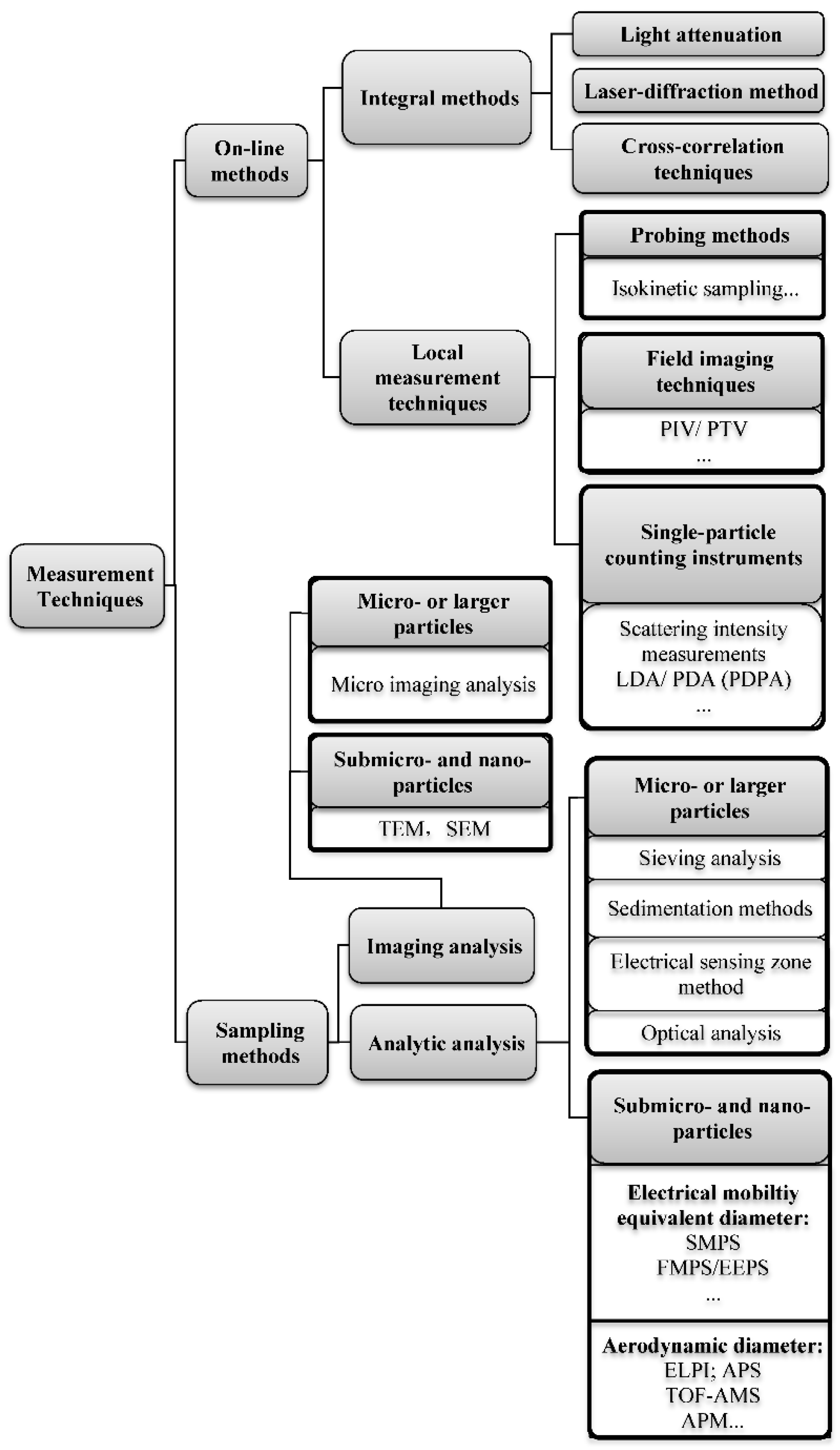
The most important measurement methods for micro- to larger particle-laden gas flows versus nano- to sub-micro-particle-laden gas flows are outlined in this section.

3.1. Optical Particle Characterization

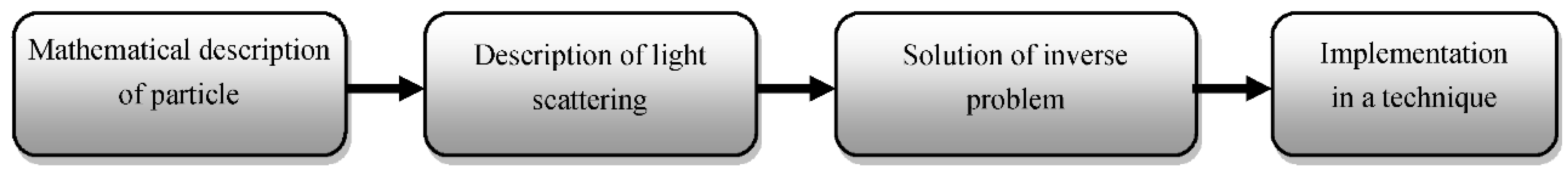
One of the most important experimental characterization methods for microparticles (or larger particles of the continuum regime) is optical analysis. Optical analysis is especially popular in two-phase flow experiments, because it is carried out as a non-intrusive on-line test, for example PIV, LDA or light-scattering techniques. At first, optical analysis was only used to measure particle velocity and number density. Now, it can analyze particle size distribution (PSD) using new laser technology, such as the phase Doppler particle analyzer (PDPA). Such techniques measure particle temperature, shape and chemical components. In spite of such recent developments, one of the ongoing challenges of such advanced measurement technologies is to assess their measurement uncertainty. The four steps involved in particle characterization using optical analysis techniques are summarized by Tropea et al. in Figure 3 [8].

The main optical particle characterization techniques are comprehensively classified according to their measurement principles and measured quantities in Tropea et al. [8] and summarized here in

Table 1. Optical analysis techniques for particle characterization.

Measurement Principle	Measured Quantity	Technique
Imaging	Velocity, particle size, shape	PIV/PTV, shadowgraphy, glare-point separation
Light intensity, light intensity ratio	Particle size, temperature, chemical composition	Extinction/absorption, modulation depth, Mie/LIF intensity ratio, dual band/three band LIF (laser-induced fluorescence)
Interferometry	velocity, particle size, refraction index/temperature	LDA, PDA, ILIDS (interferometric laser imaging for droplet size)/IPI (interferometric particle imaging), diffraction, rainbow refractometry, holography
Time shift	Particle size, velocity	The flying time, pulse displacement, time-shift technique
Pulse delay	Particle size, temperature	Femtosecond laser method
Raman scattering	Temperature, species concentration	Raman spectroscopy

. The measurement techniques listed here only cover techniques for particles larger than 500 microns (within the continuum regime or partly overlapping with the transition regime). Typically, both elastic scattering and inelastic scattering are used for optical particle characterization. Elastic scattering is used to detect particle size and velocity, while inelastic scattering is used to measure particle temperature, density and chemical species.

In particle-laden gas flows, the relative velocity between particles and the carrier phase affects the particle concentration distribution and flux density, as well as the interphase transfer of mass and heat. This indicates that velocity measurement of both phases is indispensable. The velocity of the dispersed phase and the carrier phase can be acquired optically, either as a pointwise measurement, such as with an LDA [9], or as a field measurement, such as with PIV/PTV [3,10]. The relative velocity between phases depends not only on the particle velocity, but also on the velocity of the carrier phase. This suggests that the velocity of the tracer particle used to deduce the carrier phase velocity and the velocity of the dispersed particle should be measured simultaneously. There are two effective solutions to this problem: (i) using a scattering light signal from the tracer and dispersed particle of a different wavelength; or (ii) ensuring there is a large size difference between the tracer and dispersed particle.

3.1.1. Particle Image Velocimetry

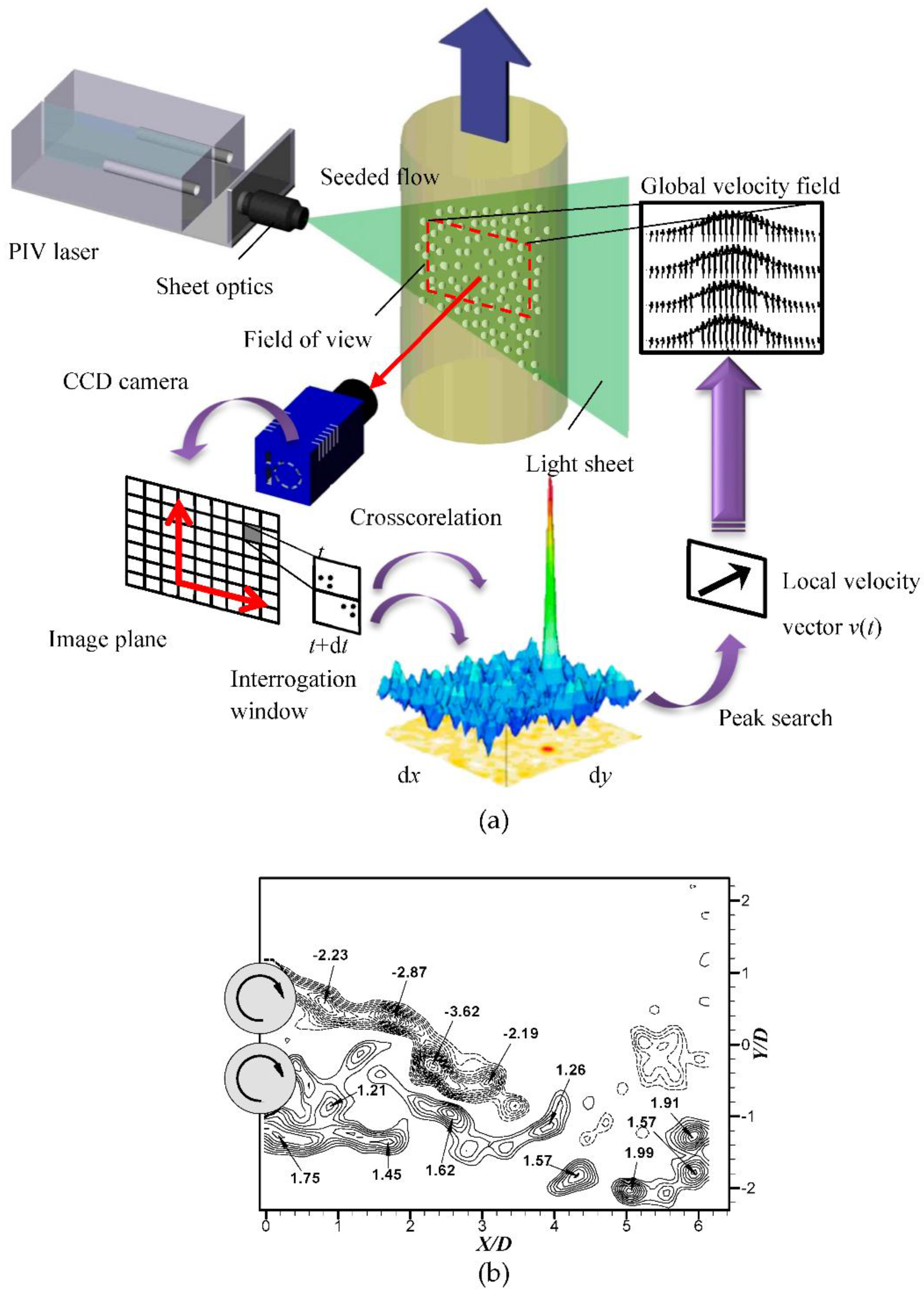
PIV is a non-intrusive measurement technique for determining the instantaneous flow field, based on a pair of time-correlated particle images having a short time lag of several to hundreds of microseconds. PIV is able to measure the velocity field, as well as other measurable quantities in real time, such as particle concentration distribution and temperature. Thus, PIV has been widely applied to fields as diverse as aerospace propulsion, biomedicine, aeronautics and micro-electromechanical systems (MEMS). During a typical PIV measurement, the tracer particles are first broadcast into the fluid and excited by a laser pulse, so that the scattered light from these particles is recorded using a CCD. The laser pulse and the CCD are triggered synchronously. Pairs of particle images are shot at short time intervals. The particles’ shifts can be calculated using cross-correlation or self-correlation, while the velocity vector of the interrogation window is calculated by averaging the entire particles’ shifts within the image area. Finally, a velocity field is reconstructed, after determining all velocity vectors. Figure 4 outlines the steps involved in the PIV technique.

In the early 1980s, it was shown by Meynart [11] that PIV could be used for the measurement of flow fields. Over the last 20 years, techniques using analog image acquisition and post-processing have been gradually replaced by techniques using digital image capture, such as CCD [3]. Because PIV is popular for fluid mechanical studies, there are abundant reviews on the various advances in PIV, outlined in

Table 2. Relevant reviews of advances in particle image velocimetry over time.

Times	Authors	Reference
Before 1990	Lauterborn and Vogel (1984) [12] Adrian (1986, 1991) [13,14]	“Modern optical techniques in fluid mechanics”, Ann. Rev. Fluid Mech., vol. 16, no. 16, pp. 223–244, 1984. “Multi-point optical measurements of simultaneous vectors in unsteady flow—a review”, Int. Journal of Heat and Fluid Flow, vol. 7, no. 2, pp. 127–145, 1986. “Particle-imaging techniques for experimental fluid mechanics”, Ann. Rev. Fluid Mech., vol. 23, no. 23, pp. 261–304, 1991.
In the 1990s	Adrian (1996) [15] Grant (1997) [16]	Bibliography of particle image velocimetry using imaging methods: 1917–1995, TAM Report 817, UILU-ENG-96-6004, University of Illinois (USA), 1996. “Particle image velocimetry: a review”, Proc. Inst. Mech. Eng. C, vol. 211, no. 1, pp. 55–76, 1997.
After 2000	Adrian (2005) [17]	“Twenty years of particle image velocimetry”, Exp. Fluids, vol. 39, no. 2, pp. 159–169, 2005.

.

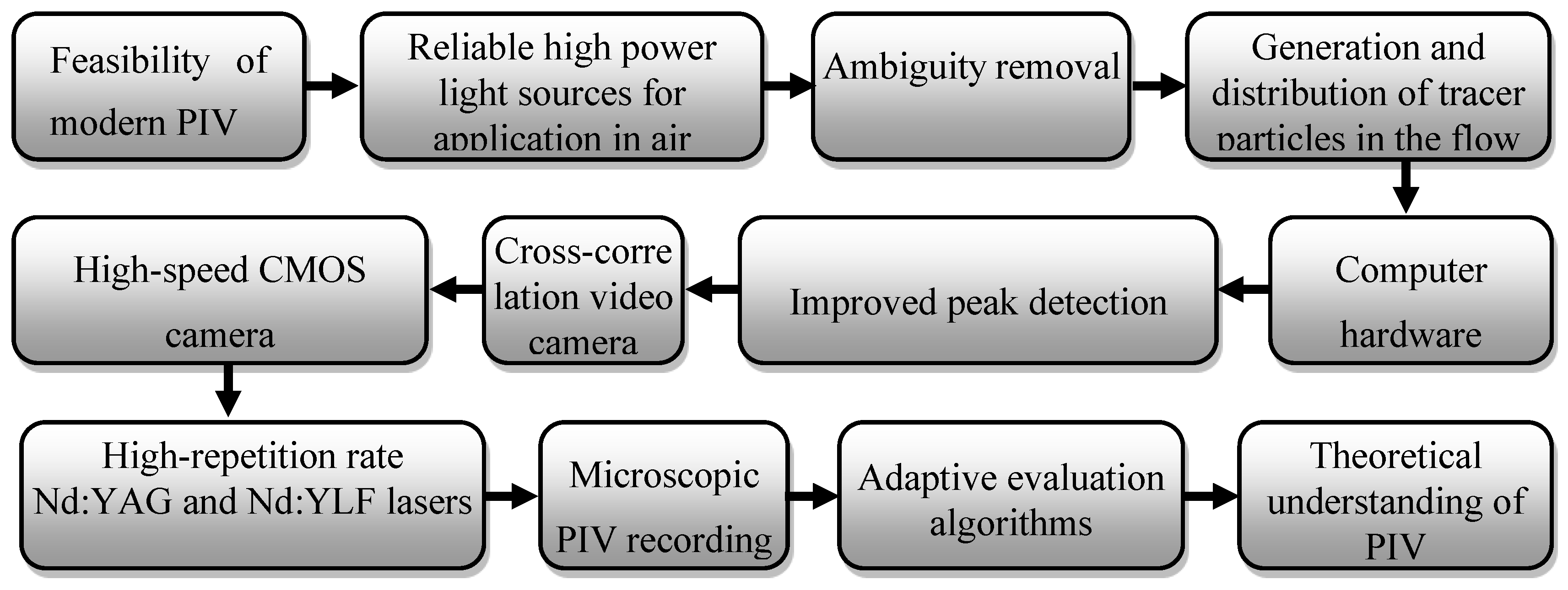
The references covered in each of these reviews total more than 100, and there are more than 1200 references on PIV published from 1917 to 1995 collated by Adrian. The major technical advances over the last 30 years for this technique were presented by Raffel et al. [3], as shown in Figure 5. Most recently, high-time resolution PIV and holographic PIV methods have been commercialized, supported by CMOS cameras and high-repetition rate Nd:YAG and Nd:YLF lasers.

The measurement of instantaneous velocity fields using PIV, effectively pushed forward research on unsteady flow, with PIV results able to directly verify the numerical results of computational fluid dynamics. Since its appearance, PIV has gradually displaced LDA, because it is able to examine the velocity of both the dispersed and carrier phases. At low particle concentrations, a normal laser is sufficient to scatter light from relatively large particles in the continuum regime, and high-contrast particle images can be captured using a basic camera. In cases with high particle concentrations or large imaging areas, there are probably several particles in each interrogation area, making conventional digital cross-correlation PIV quite practical. If particle concentration is so low that each interrogation area only includes one particle, then PTV can be used to explore the particle trajectory and velocity using a Lagrangian approach. It is difficult to measure the velocity of the carrier phase using PIV, where there is interruption of the dispersed phase, as is the case for LDA. Examples of simultaneous measurement of two-phase flow using PIV are described in detail in Kiger and Pan [19] and Khalitov and Longmire [20]. Usually, it is possible to distinguish the dispersed-phase particles from tracer particles using obvious differences in size and luminosity, especially when the tracer particle is small enough [19,21]. However, some issues exist; for example, when tracer particles are in shadows behind extremely large particles, the camera does not capture them. Based on a technique proposed by Sakakibara [21], Paris and Eaton [22] used a low signal threshold to eliminate noise from the images and an object-growing algorithm to reduce halo effects around particles; thus, larger particles were more easily identified. Measuring the carrier-phase velocity very close to the particle surface is still one of the most difficult issues in experimental studies. This is because tracer particle images near the particle surfaces are usually eliminated as image noise. Tanaka and Eaton [23] adopted a very-high resolution PIV system, with an image area of only 3.7 mm × 4.7 mm to mitigate this problem. Theoretically, phase discrimination based only on particle image size causes errors related to zero crosstalk. Despite this improvement, the measurement area was so small that hundreds of particle image pairs were required to achieve adequate turbulence statistics.

In short, high-spatial resolution PIV techniques are the most effective experimental method for particle-laden flows with low volumetric concentrations, while high-time resolution PIV and holographic PIV techniques show great potential for turbulence analysis and three-dimensional pressure field reconstructions. However, ongoing technological progress is required, before robust testing technologies are developed [24]. In reality, micro-PIV still fails to measure microscale gas flows accurately; thus, it has a long way to go before reliable measurements can be acquired for microparticle-laden gas flows.

3.1.2. Laser Doppler Anemometry and the Phase Doppler Analyzer

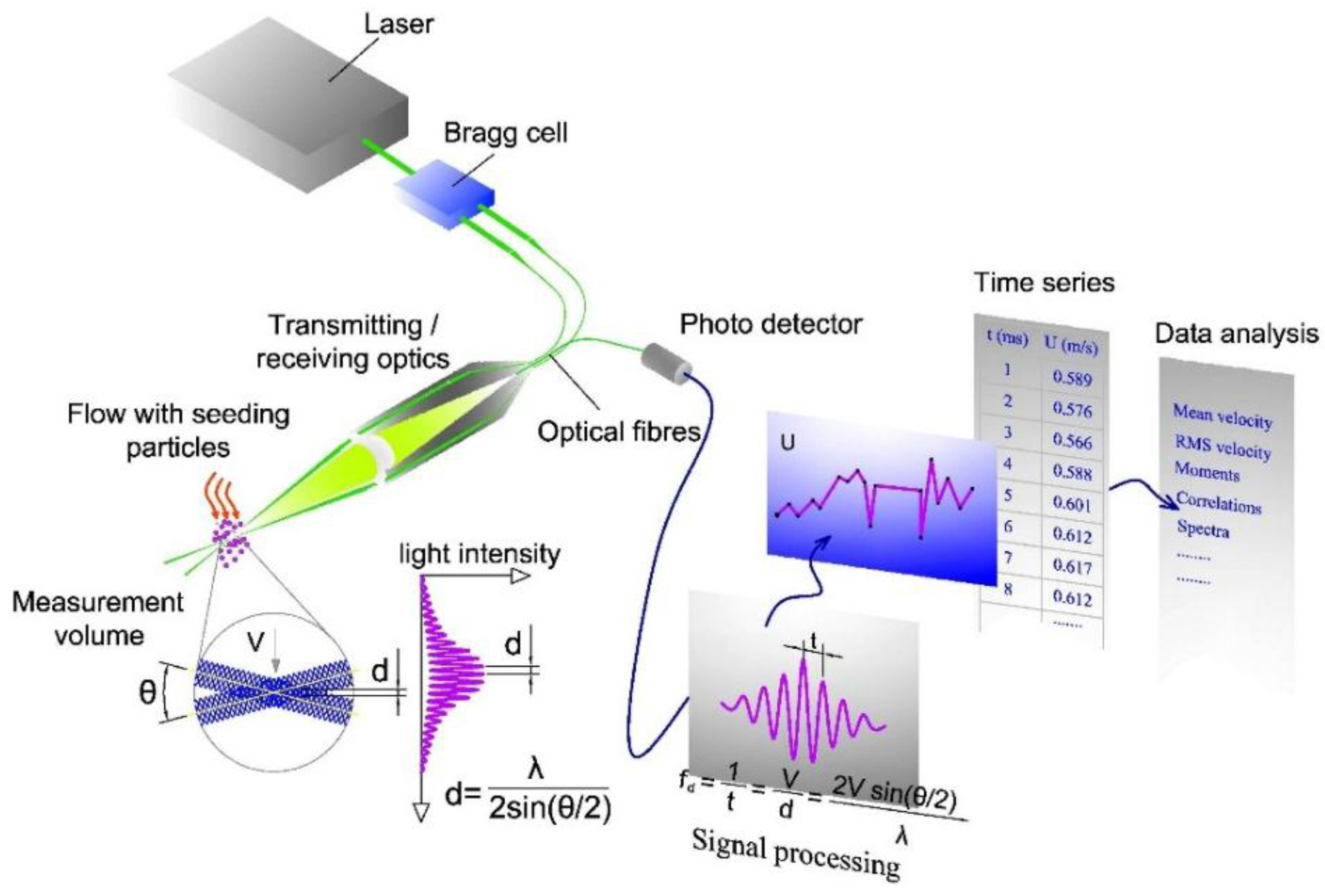
As with PIV, LDA is a non-intrusive online measurement technique, with pointwise detection based on light interference. In LDA measurements, two laser beams having similar wavelengths are induced to a focus, forming a small measurement volume. A slight frequency shift generated using a Bragg cell results in interference fringes near this focus. The interference of the two laser beams leads to alternate bright-dark fringes, reflecting the intensity modulation. These fringes are parallel to the angular bisector of the incident laser beams. According to the plane wave theory, the width of these interference fringes is given by:

$$d=\frac{\lambda }{2\sin \frac{\theta }{2}}$$

(3)

where d is the interference fringe width, λ is the wavelength of the incident laser beams and θ is the angle between the two incident beams. As a tracer particle crosses these fringes, the scattered light intensity is strongest in the bright fringes and weakest in the dark fringes. This light scattering is measured, producing a modulation signal with a Doppler shift, which is directly proportional to the particle velocity component perpendicular to the angular bisector of the incident beams, as described in Equations (4) and (5).

$$f_D=\frac{1}{t}=\frac{U_p}{d}$$

(4)

$$f_D=\frac{2\sin (\raisebox{1ex}{$\theta $}\!\left/ \!\raisebox{-1ex}{$2$}\right.)U_p}{\lambda }\iff U_p=\frac{1}{2}\frac{f_D\lambda }{\sin \left(\raisebox{1ex}{$\theta $}\!\left/ \!\raisebox{-1ex}{$2$}\right.\right)}$$

(5)

where f_D is the Doppler shift, t is the transition time to cross a fringe and U_p is the particle velocity component perpendicular to the angular bisector of the incident beams. Photomultipliers transform the fluctuations in the scattering intensity into an electrical signal of Doppler pulses. This signal is filtered and amplified using a signal processor, and the Doppler shift is obtained from spectral analysis of the processed digital signal using FFT, as shown in Figure 6. Therefore, the particle velocity component can be calculated using Equation (5). Similarly, two other velocity components can be measured using supplementary laser beam pairs of different wavelength. The scattering intensity distribution for a spherical particle predicts that the photodetector would receive the most powerful scattering signal when placed in front of the incident beams, with a 0° scattering angle. An LDA system with this configuration is called a forward LDA, whereas a backward LDA has the incident laser and photodetector on the side having the weakest signal.

The principle of the LDA may be described in the other way using the Doppler effect, which indicates the change in frequency or wavelength of sound or light for an observer moving relative to its emitter. In LDA, a moving particle receives the plane light waves, which are emitted from laser beams, and transmits them to the stationary photodetectors simultaneously. This process leads to an additional Doppler shift when the scattered light is received from a stationary observer. Then, the frequency of light received at the photodetector can be given by:

$$f_r=f_e\frac{1-\frac{\overrightarrow{v}\cdot \overrightarrow{l}}{c}}{1-\frac{\overrightarrow{v}\cdot \overrightarrow{k}}{c}}$$

(6)

where f_e is the frequency of the laser source, $\overrightarrow{v}$ is the velocity of the moving particle, c is the velocity of the light and $\overrightarrow{k}$ and $\overrightarrow{l}$ are unit vectors in the direction of the incident light and the direction of the light transmitted from the particle to the receiver.

The frequency shift f_D resulting from the scattered lights, which are obtained from two incident beams, can be expressed as:

$$f_D=f_{r1}-f_{r2}$$

(7)

Using Equation (6) and the velocity components in the directions of the two laser beams with, $|\overrightarrow{v}|\ll c$ Equation (5) is obtained again [1].

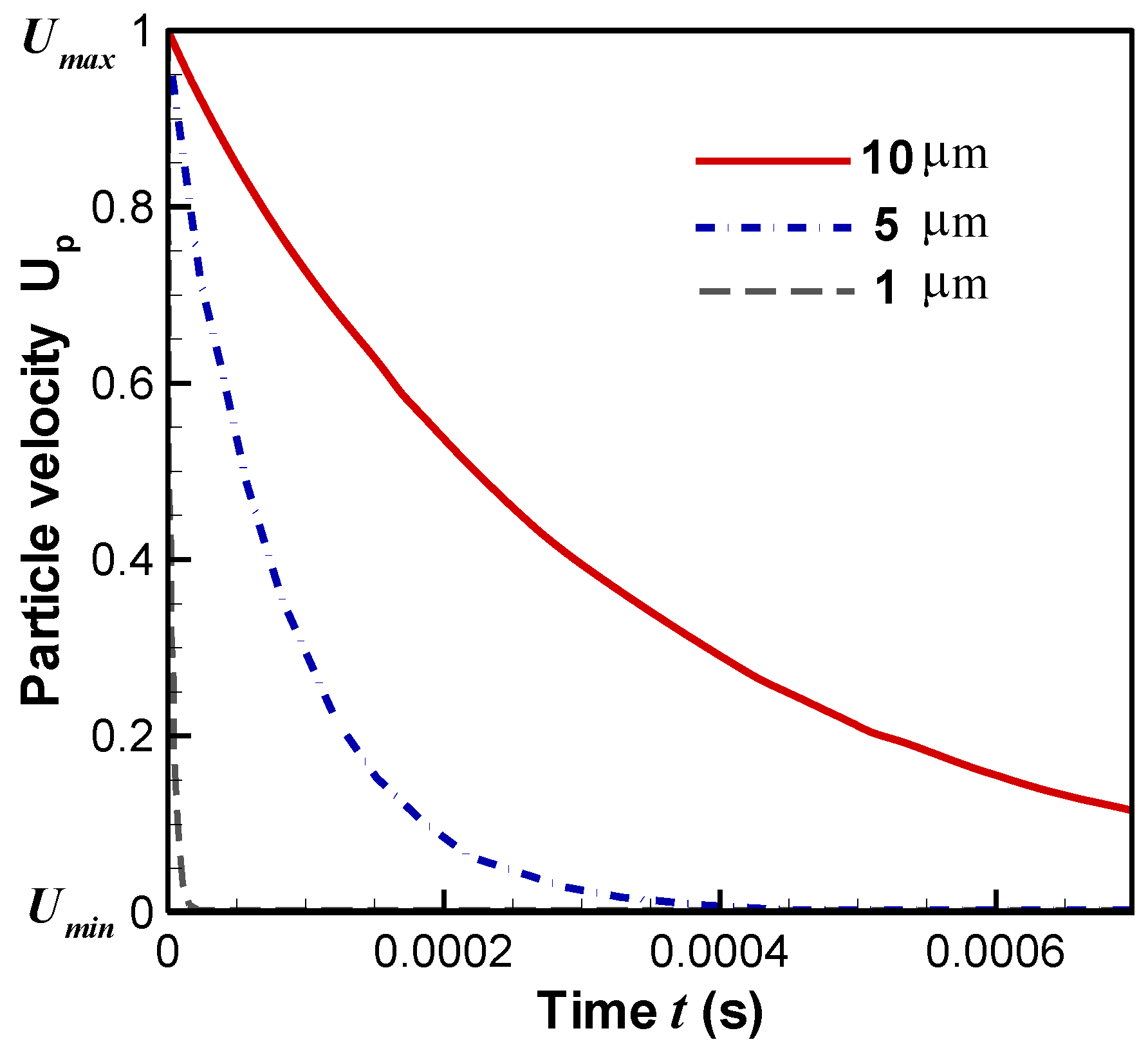
LDA has been employed to measure two-phase particle-laden gas flows for several decades. As the dispersed particles obviously need to be larger than the tracer particles, the particle scattering intensity and Doppler pulses generated also are much stronger; thus, it is very easy to measure particle velocity using LDA. In contrast, the Doppler pulses generated by the tracers are much weaker, and a phase-discrimination of the Doppler signal must be carried out to ensure the reliability of two-phase measurements. In the continuum regime, LDA seems to be the most viable option at present, given that most dispersed particles have a size range of 10 to 1000 μm, and tracer particles are approximately 1 μm sized.

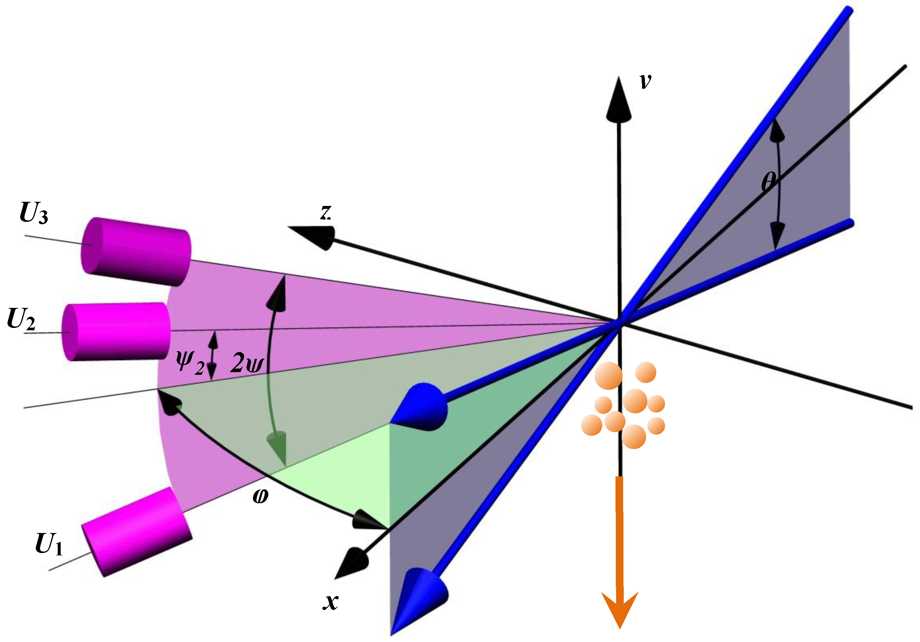
The PDA was first proposed in 1981 [25,26,27,28] as a derivative of LDA. The PDA is able to simultaneously measure spherical or quasi-spherical particle velocity and size. It has been developed into a very reliable technique for these quantities. In LDA measurements, if several detectors are used to examine the Doppler shift, then the shift signals simultaneously acquired by these detectors are similar, although there are phase-differences between them that are proportional to particle size, as shown in Figure 7. Taking into consideration only first-order refraction, the correlation between the phase-difference and particle size is equal to:

$$\Delta {\mathsf{\Phi }}^{(p=2)}\approx -2\frac{2\pi }{\lambda }{d}_p\frac{m\sin \psi \sin \raisebox{1ex}{$\theta $}\!\left/ \!\raisebox{-1ex}{$2$}\right.}{\upsilon \sqrt{1+m^2-m\upsilon }}$$

(8)

where ΔΦ^{(p = 2)} is the phase-difference between fringes on the two detectors, placed at elevation angles ±ψ and off-axis scattering angles of ±φ; m is the ratio (relative refractive index) of refractive indexes between the particle and the carrier phase; and v is a parameter function, described by:

$$\upsilon =\sqrt{2}\sqrt{1+\cos \psi \cos \phi \cos \theta /2}$$

(9)

A proportional relationship between the measured phase difference and particle diameter was found to be affected by the proportionality constant, involving geometric quantities [8]. Thus, the PDA technique is usually considered to be calibration free and in situ traceable, although its overall accuracy depends on the precision of the angles, as seen in Equation (8). The PDA is most suitable for measuring liquid and transparent droplet diameter and velocity, because first-order refractive light is often the target signal in PDA measurements. However, spherical transparent solid particles also can be measured using PDA, and even opaque spherical particles can be discriminated, using reflective light as the target signal.

Phase-Doppler techniques use a full-featured instrument that detects particles down to 300 nm in diameter (based on the detector sensitivity), for concentrations ranging from 10⁴ to 10⁵ particles/cm³. When particle size is larger than the measurement volume, it is difficult to discriminate first-order refractive light from reflective light, because of mixing. Hence, any determination of particle size directly calculated from the Doppler phase difference would result in significant error. Saffmann [29] first observed this phenomenon, although this Gaussian beam effect/defect has been studied by other authors [30,31,32]. A number of studies have focused on reducing this error to increase the viable particle concentration range [30,33].

3.1.3. Scattering Intensity Measurements

Particle characterization (e.g., particle size and concentration) using scattering intensity measurements is a long-standing technology for multiphase flow, which was well known and widely used before the emergence of either LDA/PDA or PIV. 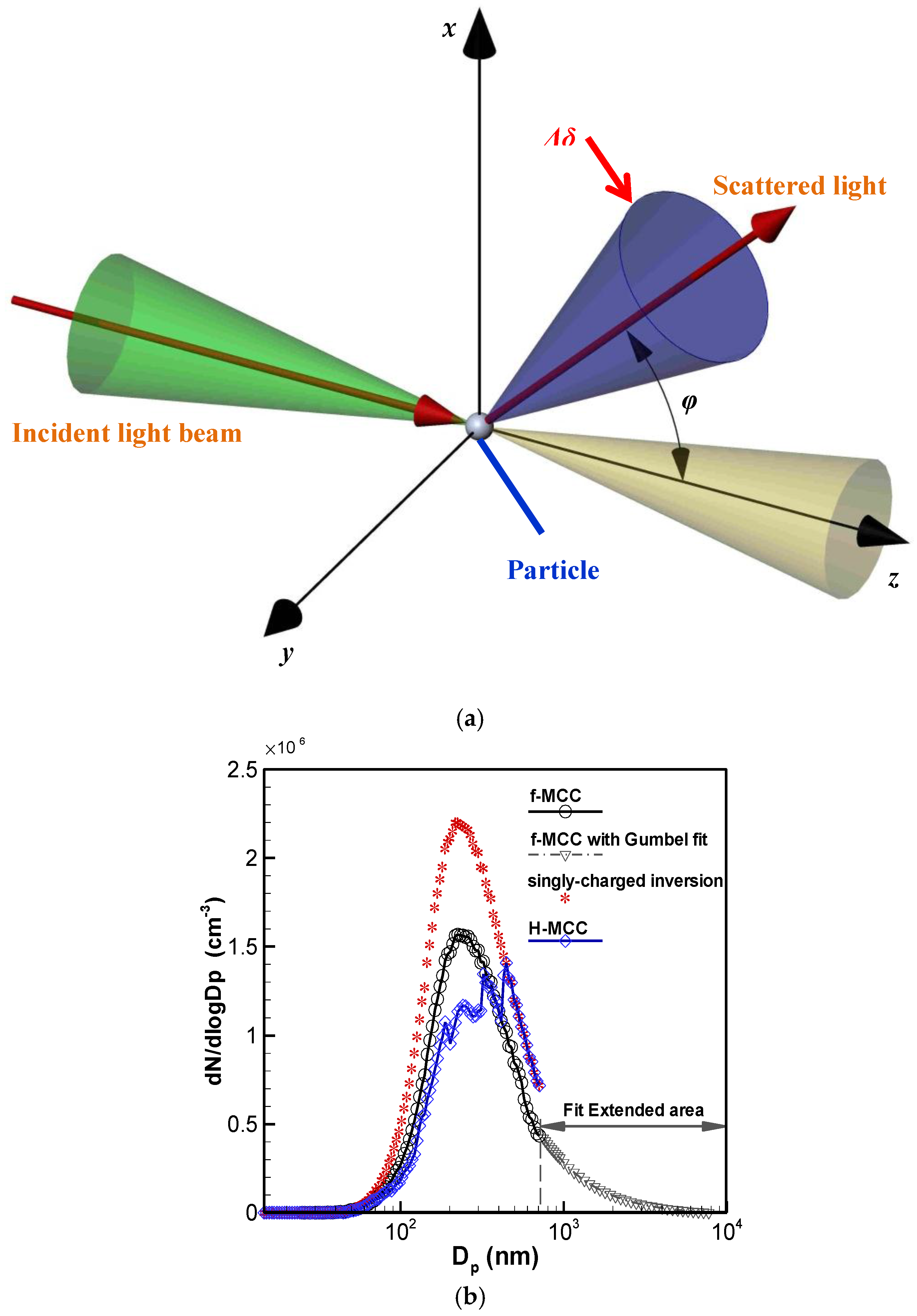Recently, scattering intensity measurements combined with laser or fluorescence illumination have extended the particle characteristics able to be detected in this technique, e.g., particle velocity [34,35], temperature [36,37] and chemical species [38]. It is used not only to detect micro- or larger particles, but also to measure nano-particle concentrations, e.g., in condensation particle counters, and a practical result obtained using this technique is shown in Figure 8b. The optical principles behind scattering intensity measurements are shown in Figure 8a. The signal received from the optical measurement system is usually equal to the integral of the scattering intensity on the receiving aperture of the optical sensor. In this case, φ is the scattering angle (the receiving angle of the photoelectric detection system), and Δδ is the receiving solid aperture angle. Under parallel and monochromatic light, with a scattering angle φ, the scattering intensity is equal to:

$$Q\left(\lambda ,d_p,m_0,\kappa ,\Delta \delta \right)=I_0\frac{{\lambda }^2}{8{\pi }^2}{\displaystyle {\int }_0^{2\pi }{\displaystyle {\int }_{\Delta \delta }I\left(\lambda ,\gamma ,\phi ,d_p,m_0,\kappa \right)}}\sin \phi d\phi d\gamma$$

(10)

where Q is the scattering intensity received by the detector, κ and m₀ are the particle complex refractive index coefficients and I₀ is the incident light intensity. This equation indicates that the scattering intensity depends on the optical arrangement constants, as well as the particle refractive index.

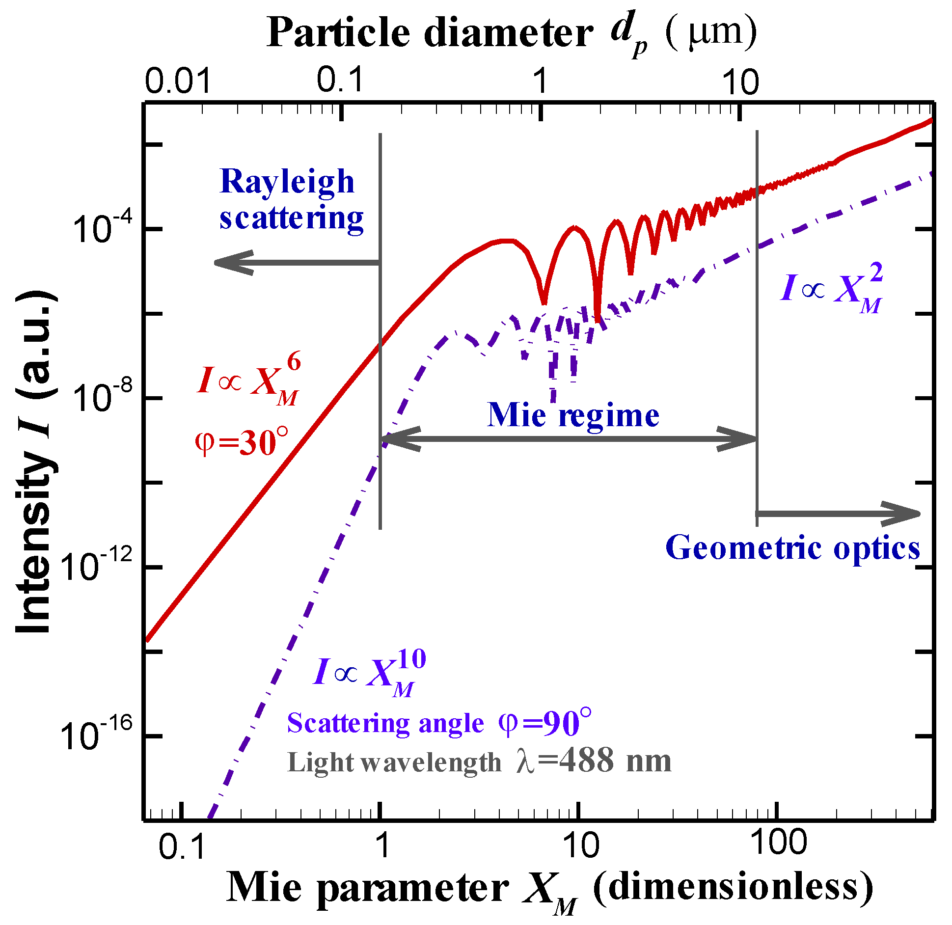
There are three fundamental scattering mechanisms for a water droplet in air: Rayleigh scattering, Mie scattering and geometric optics, depending on the particle size and its related scattering intensity, as shown in Figure 9. Here, X_M is the Mie parameter X_M = d_pπ/λ, which is equivalent to the dimensionless particle diameter for Mie scattering, for parallel polarized light and complex refractive index m = 1.333 + i0.313. This relationship indicates that particle scattering intensity is basically proportional to the dimensionless particle diameter (X_M) for Rayleigh scattering and geometric optics. This yields values of $X_M^6$ and $X_M^{10}$ for scattering angles of 30° and 90°, respectively, under Rayleigh scattering; but $X_M^2$ for both scattering angles under geometric optics. This linear relationship is critical for determining particle diameter from scattering intensity measurements, although it is difficult to do this for Mie scattering, because of its non-monotonic and highly fluctuating relationship between X_M and I. However, there are modifications available to deal with this problem, such as expanding the receiving aperture area, using a white light source or setting the scattering angle to 0° to smooth Mie scattering, as particle size increases [1]. For $d_p\gg \lambda$, the particle scattering intensity is strongest at a 0° scattering angle, because diffracted light is dominant, compared with the other two scattered light components (externally-reflected and internally-refracted light), and is highly concentrated in a forward scattering direction. This regime of geometrical optics is termed the Fraunhofer diffraction regime. In this regime, the particle scattering intensity only depends on the incident light wavelength and particle size; thus, increases in particle size decrease the angular range of the diffracted light. In this case, the diffracted light intensity is independent of the optical constants of the particle material and may be used to measure particles of different or undetermined refractive indices. In contrast to a 0° scattering angle, a scattering angle of 90° usually produces the weakest scattered light and receiving light signal. However, in practice, limited operating space and the requirement of non-intrusive detection usually results in setups having $\phi ={90}^{\circ }$. Given that there should be only one particle in the measurement volume to avoid significantly overestimating particle size, this determines the upper concentration limit of the scattering intensity techniques. There are two ways to solve this problem: (1) use a microparticle-laden gas flow with particles smaller than the measurement volume, which can be generated using a micro-mechanical device, e.g., a particle-laden micro-jet flow in a particle counter, although this involves a sampling stage; and (2) use an optical arrangement that achieves a small enough measurement volume, which can be carried out online.

Other parameters, such as tracer particles and blockages of incident light or scattered light, also have a marked effect on particle characterization using scattering intensity measurements. It is important to note that scattering intensity measurement techniques inevitably fail to characterize particles in the Mie scattering regime, because of their non-monotonic relationship with dimensionless diameter X_M and scattering intensity I. Mie/laser-induced fluorescence (LIF) ratio technology was specifically developed to overcome this problem [40,41,42,43]. In this technique, the ratio of fluorescence intensity to scattered light is used as an analog signal to replace the conventional scattering intensity. Using fluorescent tracers, it is presumed that fluorescence intensity is proportional to droplet volume (d_p³), while Mie scattering intensity is proportional to d_p²; thus, the intensity of fluorescence and Mie scattering can be distinguished according to their varied wavelengths, and particle size can be estimated using their intensity ratio. This method has reduced the influence of other parameters on the detection, but leads to a dependence on particle size and fluorescent concentration, as well as any related calibration. Currently, only droplets can be characterized using Mie/LIF ratio measurements, since there are still several unresolved issues for measuring solid particles and non-spherical particles.

3.1.4. Laser-Induced Fluorescence Techniques for Temperature and Composition Measurements

LIF is derived from a process that begins with the absorption of the incident light by the fluorescent molecules, which are activated to a higher energy level. Some of the excited molecules return to the ground state by emitting fluorescence. As one of the most important inelastic scattering techniques, laser-induced fluorescence (LIF) is also used to measure particle temperature [36] and composition [38]. The basic principle behind such techniques rests on the temperature or molar fraction dependence of the fluorescence quantum yield.

The fluorescence intensity detected on a spectral band from a droplet, which is previously seeded with a low concentration fluorescent tracer, is given by [36]:

$$I_{\mathrm{f}i}={\displaystyle {\int }_{{\lambda }_{i1}}^{{\lambda }_{i2}}{K}_{\mathrm{opt}}\left(\lambda \right)K_{\mathrm{spec}}\left(\lambda \right)}{V}_C{I}_{0}C{\mathrm{e}}^{\beta \left(\lambda \right)/T}d\lambda \approx K_{\mathrm{opt}i}{K}_{\mathrm{spec}i}{V}_C{I}_{0}C{\mathrm{e}}^{\frac{ai}{T}+\frac{bi}{T^2}}$$

(11)

where f denotes the fluorescence, i denotes the spectral band, K_opt is an optical constant specific to the optical device, K_spec is a constant that depends solely on the spectroscopic properties of the fluorescent tracer in its environment, I₀ is the laser excitation intensity, C is the molecular tracer concentration, T is the absolute temperature, V_C is the collection volume of the fluorescence photons, β(λ) describes the temperature dependence of the fluorescence intensity at the wavelength λ and a and b are the temperature sensitivity coefficients for the spectral band i. 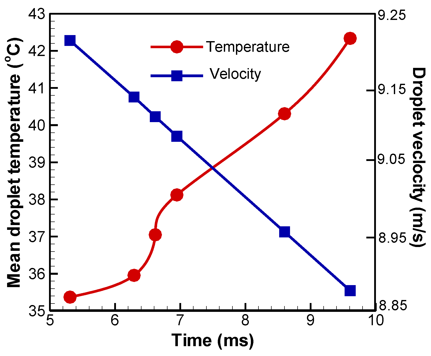However, the I₀, V_C and C are strongly dependent on the droplet size, droplet position and on the probe volume dimensions. In order to address these problems, Lavieille et al. determine the fluorescence intensity on two spectral bands (called two-band LIF) for which the temperature sensitivity is significantly different, and the selection of these spectral bands is optimized. Then, the temperature can be calculated from the fluorescence ratio between both fluorescence intensities collected on both optimal spectral bands [36]:

$$R_{\mathrm{f}}=\frac{I_{\mathrm{f}1}}{I_{\mathrm{f}2}}=\frac{K_{\mathrm{opt}1}}{K_{\mathrm{opt}2}}\frac{K_{\mathrm{spec}1}}{K_{\mathrm{spec}2}}{\mathrm{e}}^{\frac{a_1-a_2}{T}+\frac{b_1-b_2}{T^2}}$$

(12)

Mean droplet temperature and velocity evolution in the flame as a function of time are plotted in Figure 10 [36].

The fluorescence quantum yield g should rely on the liquid phase composition (i.e., fluorescent tracer fraction and temperature). However, Maqua et al. showed that the variation of g is almost negligible in the temperature range of the liquid phase [38]. Consequently, the total emitted fluorescence can be used to detect the number of molecules of the fluorescing component in a droplet, and the relation between the fluorescence signal and molar fraction of fluorescent tracer χ_a (i.e., acetone), which is strongly related to g, can be expressed by:

$$I_{\mathrm{f}}=K_{\mathrm{opt}}{K}_{\mathrm{spec}}{I}_1\mathrm{d}V{\chi }_a\frac{1}{{\chi }_a\mu +1}$$

(13)

where I_l is the local intensity, which can be related to the laser incident intensity I₀ by Beer’s absorption law, dV is an elementary volume and μ is a dimensionless empirical constant, which can be properly calibrated in the experimental procedure.

3.2. Experimental Methods for Sub-micro- and Nano-particle Laden Gas Flow

Submicron- and nanometer-sized particle-laden gas flows are a common phenomenon in nature and also have been widely studied in the context of many engineering problems, including advanced nanomaterial manufacture, engineering thermophysics, chemical engineering, inhalation toxicology, medical and pharmaceutical manufacturing [44,45,46,47]. Thus, it is very important to study sub-micro- and nano-particle-laden flows to provide theory, models or measurement techniques for these engineering problems. As described above, the scattering ranges of sub-micro- and nano-particles are mainly within the Rayleigh and Mie scattering regime, in which particle scattering intensity is so weak that light signals cannot be reliably acquired by current apparatuses. However, scanning electron microscopy (SEM) and transmission electron microscopy (TEM) can capture the sub-micro- and nano-particle morphology, as they are sampled on substrates (e.g., holey carbon support films). Moreover, the very slight inertia of submicron- and nanometer-sized particles results in the invalidation of particle sieving, using mechanical or aerodynamic methods. The measurement techniques for nano-particles usually require sampling, and to date, no online technique (e.g., for measuring nano-particle velocity) has emerged. It is important to note that the particle diameter acquired using present nano-particle sizers is either an aerodynamic or an electrical mobility diameter; in which case, the electrical mobility diameter of a real spherical or non-spherical test particle is the mobility-equivalent diameter of an ideal spherical particle. Likewise, the aerodynamic diameter of a test particle is the inertia- and settling-velocity-equivalent diameter of an ideal spherical particle in air, with a density of 1000 kg/m³. Nano-particles are fantastic tracers, even in the supersonic and hypersonic boundary layer, because of their small size and inertia. Yi et al. [48] used nano-particle tracers in optical flow methods to study compressible turbulence structures at high temporal-spatial resolution. However, this comprehensive technology merely estimates the ensemble-average characteristics of nano-particles, but not its single particle ones.

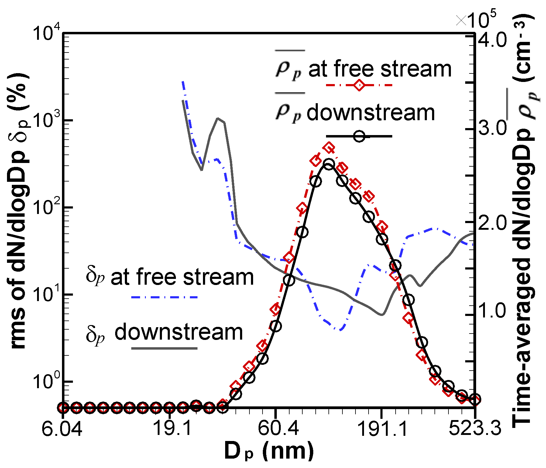
An SMPS or scanning electrical mobility spectrometer (SEMS) [49], FMPS and electrical low pressure impactor (ELPI) are three of the most widely-used commercial measuring instruments used to characterize the concentration and distribution of submicron- and nanometer-sized particles, especially for studying aerosols and particle-laden flows [47,50,51]. A general particle size distribution measured using FMPS is presented in the Figure 11, while the practical results of SMPS are shown in Figure 8. Both SMPS and FMPS characterize particle size depending on the mobility of a charged particle passing through a cylindrical electric field. In an SMPS, sampled particles are first neutralized using a bipolar charger (e.g., Kr85 or soft X-ray) in a neutralizer to attain a well-defined steady-state distribution of positively- and negatively charged-particles [2,52,53]. In contrast, particles in a FMPS are successively charged, using a negative and a positive unipolar corona charger to achieve a predictable charge distribution. A theoretical model to describe the particle charge distribution in an SMPS neutralizer was proposed by Wiedensohler [52], which is based on an approximation of Fuchs’ diffusion theory for submicron- and nanometer-sized particles [2]. The fractions of particles carrying different amounts of charge, according to this model, are given by:

$$f_c\left(N\right)={10}^{\left[{\displaystyle \sum _{i=0}^5{a}_i\left(N\right){\left(\log \frac{D_p}{nm}\right)}^i}\right]}$$

(14)

under the conditions of 1 nm ≤ D_p ≤ 1000 nm, N = −1, 0, 1; or 20 nm ≤ D_p ≤ 1000 nm, N = −2, +2; and:

$$f_c\left(N\right)=\frac{e}{\sqrt{4{\pi }^2{\epsilon }_0{D}_{p}KT}}\exp \frac{-{\left[N-\frac{2\pi {\epsilon }_0{D}_{p}KT}{e^2}\ln \left(\frac{Z_{i+}}{Z_{i-}}\right)\right]}^2}{2\times \frac{2\pi {\epsilon }_0{D}_{p}KT}{e^2}}$$

(15)

for the fraction of particles carrying three or more charges.

Here, N is the number of elementary charges on a particle; a_i is a coefficient related to N; T is the temperature; and all other physical constants are listed in

Table 3. Relevant physical constants for modeling the charge distribution of submicron- to nanometer-sized particles.

Physical Constants	Definition	Value	Units
e	elementary charge units	e = 1.60217733 × 10-19	C
${\epsilon }_0$	Dielectric constant	${\epsilon }_0=8.854187817\times {10}^{-12}$	(F/m)
K	Boltzmann’s constant	K = 1.380658 × 10-23	(J/k)
$z_{i+}/z_{i-}$	ion mobility ratio	$z_{i+}/z_{i-}=0.875$

.

The sampled particles are classified according to their differential electrical mobility in both the SMPS and the FMPS or their characteristic aerodynamic diameter in the ELPI. Because particle density clearly has a huge influence on ELPI measurements, particle density needs to be known to use this technique.

The DMA in a SMPS, used to classify the particles, usually consists of two cylindrical electrodes made of polished stainless steel [54], in which the resulting drag force on the charged particle can quickly increase and become equal to the electrical force. According to the Stokes law, the neutralized particles following a steady-state charge distribution will achieve different terminal velocities related to their experience of the electrical force and the drag force in the annular electrical field. This produces a specific electrical mobility in the particle that determines whether it meets the conditions outlined in Equation (16) and enters the DMA, as the presupposed particle size to be measured.

$$\frac{d_p}{C_c\left(d_p\right)}=\frac{2NeVL}{3\mu q_{sh}\ln \frac{R_1}{R_2}}$$

(16)

where d_p is the particle electrical mobility equivalent diameter, q_sh is given by q_sh = (Q_sh + Q_ex)/2, Q_sh is the sheath air flow rate, Q_ex is the excess flow rate, V is the average voltage on the inner central rod, L is the length between the exit slit and the polydisperse aerosol inlet, R₁ is the inner radius of the annular space, R₂ is the outer radius of the annular space, C_c is Cunningham slip correction and μ is the gas dynamic viscosity. Equation (16) also indicates that monodisperse particles of a defined diameter can be attained by accurately adjusting V. These monodisperse aerosols are transported into a concentration detector, e.g., a concentration particle counter [55] or electrometer [56,57], to characterize particle concentration. It usually takes an SMPS several minutes to analyze each size distribution, with sizes ranging from 2.5 nm to 1000 nm, because it needs to scan through all size channels. The size resolution of an SMPS has increased to cover up to 64 channels, making its size resolution one of the highest among these three techniques.

In contrast to an SMPS, the outer cylinder in an FMPS classifier is divided into several electrically isolated segments, which are monitored using individual electrometers [58]. Particles in well-defined charge states will collide against the outer cylinder at different electrometers, based on their electrical mobility, i.e., particles of lower electrical mobility will collide against electrometers closer to the outlet than ones with higher mobility. Hence, the current received by each electrometer can be used to reconstruct the number size distribution of the sampled particles. An FMPS does not need to scan through various voltages; hence, it has a time resolution of about 1 s for each size distribution in the size range of 5 nm to 560 nm.

Similar to an FMPS, particles in an ELPI are first charged in a unipolar charger. However, unlike the SMPS and the FMPS, the ELPI [59] classifies sampled particles using a cascade low-pressure impactor, which is connected to individual electrometers. Particles impacting on a collection plate are deposited on the plate; thus, the charges on the plates generate currents related to their particle concentration. Both size and time resolutions of the ELPI are close to the FMPS, with a size resolution based on 14 channels and a time resolution of about 1 s. Moreover, it can measure high-temperature aerosols and is most commonly used in energy engineering for particles having a size range of 6 to 10 μm.

Both Lee et al. [60] and Christof et al. [61] found that particle size distributions (PSDs) acquired using an FMPS show a clear negative deviation from those acquired with an SMPS, although there is a strong linear relationship between these techniques. Lee et al. [58] further demonstrated that PSDs measured using various SMPSs are consistent and proposed a correction expression for PSDs detected using an FMPS. High repeatability and consistency of SMPS led to its wide application in aerosol science and various industrial processes. It has been designated a standard meteorology technique for nano-aerosol measurements in many countries. A more detailed analysis of nano-particle measurement techniques can be found in Prashant et al. [61,62].

4. Conclusions

This article reviews measurement techniques for both carrier phase and dispersed particles from the nanoscale to the microscale in size, with a focus on the developments of various techniques over the last 20 years. It also draws relationships and makes comparisons among these techniques. We provide a systematic description and classification of these optical and electrical methods and describe the parameters they measure, such as particle velocity, size, composition and concentration. A more detailed review is made of some of the most important measurement techniques, including PIV, PDPA and light scattering intensity for micro-particles, as well as the SMPS, FMPS and ELPI for nano-particles. The principles, development histories and applications of these techniques are covered. In general, their spatial and time resolutions appear to be the main factors affecting the scope of these techniques.

Despite the various effective techniques referred to in this paper, there are still several challenges to be addressed. Now that non-intrusive diagnostic techniques for the carrier phase use particles as small as the tracer particles, the influence of these tracers on the fluids needs to be considered. In particular, this needs to be addressed when micro-channel flow has sub-microparticles as tracers and when high-speed flow requires very high tracer concentrations to satisfy the camera sensitivity. Theoretical models for many of these techniques still need to be developed. For micro- or larger particles, the extension of existing particle characterization methods to non-spherical particles and non-homogeneous particles is very important for both engineering and scientific applications. For submicron- and nano-sized particles, there is a strong demand for the development of online techniques and in situ (freezing) sampling methods, which can reproduce the exact particle spatial distribution, without being affected by particle-particle interactions and particle deposition.

References

1. Crowe, C.T.; Sommerfeld, M.; Tsuji, Y. Multiphase Flows with Droplets and Particles; CRC Press: Boca Raton, FL, USA, 1998. [Google Scholar]
2. Fuchs, N.A. On the stationary charge distribution on aerosol particles in a bipolar ionic atmosphere. Pure Appl. Geophys. 1963, 56, 185–193. [Google Scholar] [CrossRef]
3. Raffel, M. Particle Image Velocimetry: A Practical Guide; Springer: New York, NY, USA, 1998; p. 216. [Google Scholar]
4. Doig, I.D.; Roper, G.H. Air Velocity Profiles in Presence of Cocurrently Transported Particles. Ind. Eng. Chem. Fundam. 1967, 6, 247–256. [Google Scholar] [CrossRef]
5. Hetsroni, G.; Sokolov, M. Distribution of Mass, Velocity, and Intensity of Turbulence in a Two-Phase Turbulent Jet. J. Appl. Mech. 1971, 38, 315–327. [Google Scholar] [CrossRef]
6. Calzavarini, E.; Berg, T.H.V.D.; Toschi, F.; Lohse, D. Quantifying microbubble clustering in turbulent flow from single-point measurements. Phys. Fluids 2008, 20, 1569–1579. [Google Scholar] [CrossRef]
7. Zhou, Y.; Yiu, M.W. Flow structure, momentum and heat transport in a two-tandem-cylinder wake. J. Fluid Mech. 2006, 548, 17–48. [Google Scholar] [CrossRef]
8. Tropea, C. Optical Particle Characterization in Flows. Fluid Mech. 2011, 43, 399–426. [Google Scholar] [CrossRef]
9. Albrecht, H.E.; Borys, D.I.M.; Damaschke, D.I.N.; Tropea, D.I.C. Laser Doppler and Phase Doppler Measurement Techniques; Springer: New York, NY, USA, 2003; pp. 9–26. [Google Scholar]
10. Estruchsamper, D. Particle Image Velocimetry, AdrianR. J. and WesterweelJ., Cambridge University Press, The Edinburgh Building, Shaftesbury Road, Cambridge, CB2 2RU, UK. 2011. 558pp. £75. ISBN 978-0-521-44008-0. Aeronaut. J. 2012, 116, 219–220. [Google Scholar]
11. Meynart, R. Mesure de champs de vitesse d’ ecoulements fluides par analyse de suites d’ images obtenues par diffusion d’ un feuillet lumineux. Ph.D. Thesis, Universite Libre de Bruxelles, Bruxelles, Belgium, 1983. [Google Scholar]
12. Lauterborn, W.; Vogel, A. Modern Optical Techniques in Fluid Mechanics. Fluid Mech. 1984, 16, 223–244. [Google Scholar] [CrossRef]
13. Adrian, R.J. Multi-point optical measurements of simultaneous vectors in unsteady flow—A review. Int. J. Heat Fluid Flow 1986, 7, 127–145. [Google Scholar] [CrossRef]
14. Adrian, R.J. Particle-Imaging Techniques for Experimental Fluid Mechanics. Fluid Mech. 1991, 23, 261–304. [Google Scholar] [CrossRef]
15. Adrian, R.J. Bibliography of Particle Velocimetry Using Imaging Methods: 1917–1995; Department of Theoretical and Applied Mechanics, University of Illinois at Urbana-Champaign: Champaign, IL, USA, 1996. [Google Scholar]
16. Grant, I. Particle image velocimetry: A review. Arch. Proc. Inst. Mech. Eng. C J. Mech. Eng. Sci. 1997, 211, 55–76. [Google Scholar] [CrossRef]
17. Adrian, R.J. Twenty years of particle image velocimetry. Exp. Fluids 2005, 39, 159–169. [Google Scholar] [CrossRef]
18. Tu, C.X.; Bao, F.B.; Huang, L. Properties of the flow around two rotating circular cylinders in side-by-side arrangement with different rotation types. Therm. Sci. 2014, 18, 1487–1492. [Google Scholar] [CrossRef]
19. Kiger, K.T.; Pan, C. PIV Technique for the Simultaneous Measurement of Dilute Two-Phase Flows. J. Fluids Eng. 2000, 122, 811–818. [Google Scholar] [CrossRef]
20. Khalitov, D.A.; Longmire, E.K. Simultaneous two-phase PIV by two-parameter phase discrimination. Exp. Fluids 2002, 32, 252–268. [Google Scholar] [CrossRef]
21. Sakakibara, J.; Wicker, R.B.; Eaton, J.K. Measurements of the particle-fluid velocity correlation and the extra dissipation in a round jet. Int. J. Multiph. Flow 1996, 22, 863–881. [Google Scholar] [CrossRef]
22. Paris, A.; Eaton, J. Measuring velocity gradients in a particle-laden channel flow. In Proceedings of the 3rd International Workshop on PIV’99, Santa Barbara, CA, USA, 16–18 September 1999; pp. 513–518.
23. Tanaka, T.; Eaton, J.K. Sub-Kolmogorov resolution partical image velocimetry measurements of particle-laden forced turbulence. J. Fluid Mech. 2010, 643, 177–206. [Google Scholar] [CrossRef]
24. Balachandar, S.; Eaton, J.K. Turbulent Dispersed Multiphase Flow. Fluid Mech. 2010, 42, 111–133. [Google Scholar] [CrossRef]
25. Bauckhage, K.; Floegel, H. Simultaneous measurement of droplet size and velocity in nozzle sprays. In Proceedings of the 2nd International Symposium on Applications of Laser Anemometry to Fluid Mechanics, Lisbon, Portugal, 2–5 July 1984; pp. 18.1.1–18.1.6.
26. Saffman, M.; Buchhave, P.; Tanger, H. Simultaneous measurement of size, concentration and velocity of spherical particles by a laser Doppler method. In Proceedings of the 2nd International Symposium on Applications of Laser Anemometry to Fluid Mechanics, Lisbon, Portugal, 2–5 July 1984.
27. Bachalo, W.D.; Houser, M.J. Phase/Doppler Spray Analyzer for Simultaneous Measurements of Drop Size and Velocity Distributions. Opt. Eng. 1984, 23, 583–590. [Google Scholar] [CrossRef]
28. FlÖgel, H.H. Untersuchung von Teilchengeschwindigkeit und TeilchengrÖße mit einem Laser-Doppler-Anemometer. Ph.D. Thesis, Universität Bermen, Bermen, Germany, 1981. [Google Scholar]
29. Saffman, M. The use of polarized light for optical particle sizing. In Proceedings of the 3rd International Symposium on Applications of Laser Anemometry to Fluid Mechanics, Lisbon, Portugal, 7–9 July 1986; p. 18-2.
30. Sankar, S.V.; Inenaga, A.S.; Bachalo, W.D. Trajectory Dependent Scattering in Phase Doppler Interferometry: Minimizing and Eliminating Sizing Errors. In Proceedings of the 6th International Symposium on Applications of Laser Anemometry to Fluid Mechanics, Lisbon, Portugal, 20–23 July 1992; p. 12.2.
31. Gréhan, D.G.; Gouesbet, G.; Naqwi, D.A.; Durst, F. Particle Trajectory Effects in Phase Doppler Systems: Computations and experiments. Part. Part. Syst. Charact. 1993, 10, 332–338. [Google Scholar] [CrossRef]
32. Albrecht, H.E.; Wenzel, M.; Borys, M. Influence of the Measurement Volume on the Phase Error in Phase Doppler Anemometry. Part 2: Analysis by extension of geometrical optics to the laser beam; Refractive mode operation. Part. Part. Syst. Charact. 1996, 13, 18–26. [Google Scholar] [CrossRef]
33. Xu, T.; Tropea, C. Improving the Performance of Two-Component Phase Doppler Anemometers. Meas. Sci. Technol. 1999, 5, 969–975. [Google Scholar] [CrossRef]
34. Frackowiak, B.; Tropea, C. Fluorescence modeling of droplets intersecting a focused laser beam. Opt. Lett. 2010, 35, 1386–1388. [Google Scholar] [CrossRef] [PubMed]
35. Frackowiak, B.; Tropea, C. Numerical analysis of diameter influence on droplet fluorescence. Appl. Opt. 2010, 49, 2363–2370. [Google Scholar] [CrossRef] [PubMed]
36. Castanet, G.; Lavieille, P.; Lebouché, M.; Lemoine, F. Measurement of the temperature distribution within monodisperse combusting droplets in linear streams using two-color laser-induced fluorescence. Exp. Fluids 2003, 35, 563–571. [Google Scholar] [CrossRef]
37. Castanet, G.; Delconte, A.; Lemoine, F.; Mees, L.; Gréhan, G. Evaluation of temperature gradients within combusting droplets in linear stream using two colors laser-induced fluorescence. Exp. Fluids 2005, 39, 431–440. [Google Scholar] [CrossRef]
38. Maqua, C.; Depredurand, V.; Castanet, G.; Wolff, M.; Lemoine, F. Composition measurement of bicomponent droplets using laser-induced fluorescence of acetone. Exp. Fluids 2007, 43, 979–992. [Google Scholar] [CrossRef]
39. Tu, C.X. Research on the Nanoparticles Cogulation and Dispersion in Shear Layers and the Related Experimental Methods; Zhejiang University: Hangzhou, China, 2015. [Google Scholar]
40. Yeh, C.N.; Kosaka, H.; Kamimoto, T. A fluorescence/scattering imaging technique for instantaneous 2D measurements of particle size distribution in a transient spray. In Proceedings of the 3rd Congress Optical Partical Sizing, Yokohama, Japan, 23–26 August 1993; pp. 355–361.
41. Jermy, M.C.; Greenhalgh, D.A. Planar dropsizing by elastic and fluorescence scattering in sprays too dense for phase Doppler measurement. Appl. Phys. B 2000, 71, 703–710. [Google Scholar] [CrossRef]
42. Domann, R.; Hardalupas, Y. Spatial distribution of fluorescence intensity within large droplets and its dependence on dye concentration. Appl. Opt. 2001, 40, 3586–3597. [Google Scholar] [CrossRef] [PubMed]
43. Domann, R.; Hardalupas, Y. A Study of Parameters that Influence the Accuracy of the Planar Droplet Sizing (PDS) Technique. Part. Part. Syst. Charact. 2001, 18, 3–11. [Google Scholar] [CrossRef]
44. Barrero, A.; Loscertales, I.G. Micro- and Nanoparticles via Capillary Flows. Fluid Mech. 2007, 39, 89–106. [Google Scholar] [CrossRef]
45. Lin, J.-Z.; Huang, L.-Z. Review of some researches on nano-and submicron Brownian particle-laden turbulent flow. J. Hydrodyn. Ser. B 2012, 24, 801–808. [Google Scholar] [CrossRef]
46. Yu, M.; Lin, J. Nanoparticle-laden flows via moment method: A review. Int. J. Multiph. Flow 2010, 36, 144–151. [Google Scholar] [CrossRef]
47. Zhu, J.; Qi, H.; Wang, J. Nanoparticle dispersion and coagulation in a turbulent round jet. Int. J. Multiph. Flow 2013, 54, 22–30. [Google Scholar]
48. Yi, S.H; Tian, L.; Zhao, Y.; He, L. The new advance of the experimental research on compressible turbulence based on the NPLS technique. Adv. Mech. 2011, 41, 379–390. [Google Scholar]
49. Tu, C.; Zhang, J. Nanoparticle-laden gas flow around a circular cylinder at high Reynolds number. Int. J. Numer. Methods Heat Fluid Flow 2014, 24, 1782–1794. [Google Scholar] [CrossRef]
50. Wang, S.C.; Flagan, R.C. Scanning electrical mobility spectrometer. Aerosol Sci. Technol. 1990, 20, 1485–1488. [Google Scholar] [CrossRef]
51. Tu, C.X.; Zhang, J.A. Characteristic distribution of submicron and nano-particles laden flow around circular cylinder. Therm. Sci. 2012, 16, 1386–1390. [Google Scholar] [CrossRef] [Green Version]
52. Wiedensohler, A. An approximation of the bipolar charge distribution for particles in the submicron size range. J. Aerosol Sci. 1988, 19, 387–389. [Google Scholar] [CrossRef]
53. Hoppel, W.A.; Frick, G.M. Ion—Aerosol Attachment Coefficients and the Steady-State Charge Distribution on Aerosols in a Bipolar Ion Environment. Aerosol Sci. Technol. 1986, 5, 1–21. [Google Scholar] [CrossRef]
54. Knutson, E.O.; Whitby, K.T. Aerosol classification by electric mobility: Apparatus, theory, and applications. J. Aerosol Sci. 1975, 6, 443–451. [Google Scholar] [CrossRef]
55. Agarwal, J.K.; Sem, G.J. Generating submicron monodisperse aerosols for instrument calibration. TSI Q. 1978, 4, 3–8. [Google Scholar]
56. Winklmayr, W.; Reischl, G.P.; Lindner, A.O.; Berner, A.; Winklmayr, W.; Reischl, G.P.; Lindner, A.O.; Berner, A. A new electromobility spectrometer for the measurement of aerosol size distributions in the size range from 1 to 1000 nm. J. Aerosol Sci. 1991, 22, 289–296. [Google Scholar] [CrossRef]
57. He, M.; Marzocca, P.; Dhaniyala, S. A new high performance battery-operated electrometer. Rev. Sci. Instrum. 2007, 78, 105103. [Google Scholar] [CrossRef] [PubMed]
58. Tammet, H.; Mirme, A.; Tamm, E. Electrical aerosol spectrometer of Tartu University. J. Aerosol Sci. 1998, 29, 315–324. [Google Scholar] [CrossRef]
59. Keskinen, J.; Pietarinen, K.; Lehtimäki, M. Electrical low pressure impactor. J. Aerosol Sci. 1992, 23, 353–360. [Google Scholar] [CrossRef]
60. Lee, B.P.; Li, Y.J.; Flagan, R.C.; Lo, C.; Chan, C.K. Sizing Characterization of the Fast-Mobility Particle Sizer (FMPS) Against SMPS and HR-ToF-AMS. Aerosol Sci. Technol. 2013, 47, 1030–1037. [Google Scholar] [CrossRef]
61. Asbach, C.; Kaminski, H.; Fissan, H.; Monz, C.; Dahmann, D.; Mülhopt, S.; Paur, H.R.; Kiesling, H.J.; Herrmann, F.; Voetz, M. Comparison of four mobility particle sizers with different time resolution for stationary exposure measurements. J. Nanopart. Res. 2009, 11, 1593–1609. [Google Scholar] [CrossRef]
62. Kumar, P.; Robins, A.; Vardoulakis, S.; Britter, R. A review of the characteristics of nanoparticles in the urban atmosphere and the prospects for developing regulatory controls. Atmos. Environ. 2010, 44, 5035–5052. [Google Scholar] [CrossRef] [Green Version]
Figure 1. Classification of methods for particle characterization in particle-laden gas flows. Abbreviations: PIV, particle image velocimetry; PTV, particle tracking velocimetry; LDA, laser Doppler anemometry; PDA, particle Doppler analyzer; PDPA, phase Doppler particle analyzer; TEM, transmission electron microscope; SEM, scanning electron microscope; SMPS, scanning mobility particle sizer spectrometer; FMPS, fast mobility particle sizer spectrometer; EEPS, engine exhaust particle sizer spectrometer; ELPI, electrical low pressure impactor; APS, aerosol particle sizer spectrometer; TOF-AMS, time-of-flight aerosol mass spectrometer; APM, aerosol particle mass analyzer.
Applsci 07 00120 g001
Figure 2. Response time of oil particles having different diameters in a decelerating air flow [1].
Applsci 07 00120 g002
Figure 3. The four steps involved in particle characterization using optical techniques.
Applsci 07 00120 g003
Figure 4. Schematic of particle imaging velocimetry (PIV) and results: (a) showing steps involved in PIV; (b) vorticity contours of the wake behind two rotating circular cylinders using PIV [18].
Applsci 07 00120 g004
Figure 5. Development of particle image velocimetry over the last two decades.
Applsci 07 00120 g005
Figure 6. Schematic showing laser Doppler anemometry.
Applsci 07 00120 g006
Figure 7. Optical configuration of the standard (three detector) phase Doppler analyzer.
Applsci 07 00120 g007
Figure 8. Schematic of scattering intensity measurements and results: (a) optical arrangement constants; (b) particle size distribution with different multiple charged correction (MCC) methods [39].
Applsci 07 00120 g008
Figure 9. Scattering intensity as a function of the Mie parameter for two scattering angles.
Applsci 07 00120 g009
Figure 10. Mean droplet temperature and velocity evolution in the flame as a function of time: mean droplet temperature measured using two-band LIF; droplet velocity measured using LDA [36].
Applsci 07 00120 g010
Figure 11. Time-averaged particle number density and its root mean square at different positions in flow around a circular cylinder using FMPS [50].
Applsci 07 00120 g011