Influence of Winkler-Pasternak Foundation on the Vibrational Behavior of Plates and Shells Reinforced by Agglomerated Carbon Nanotubes


Abstract
:
1. Introduction
2. Theoretical Model
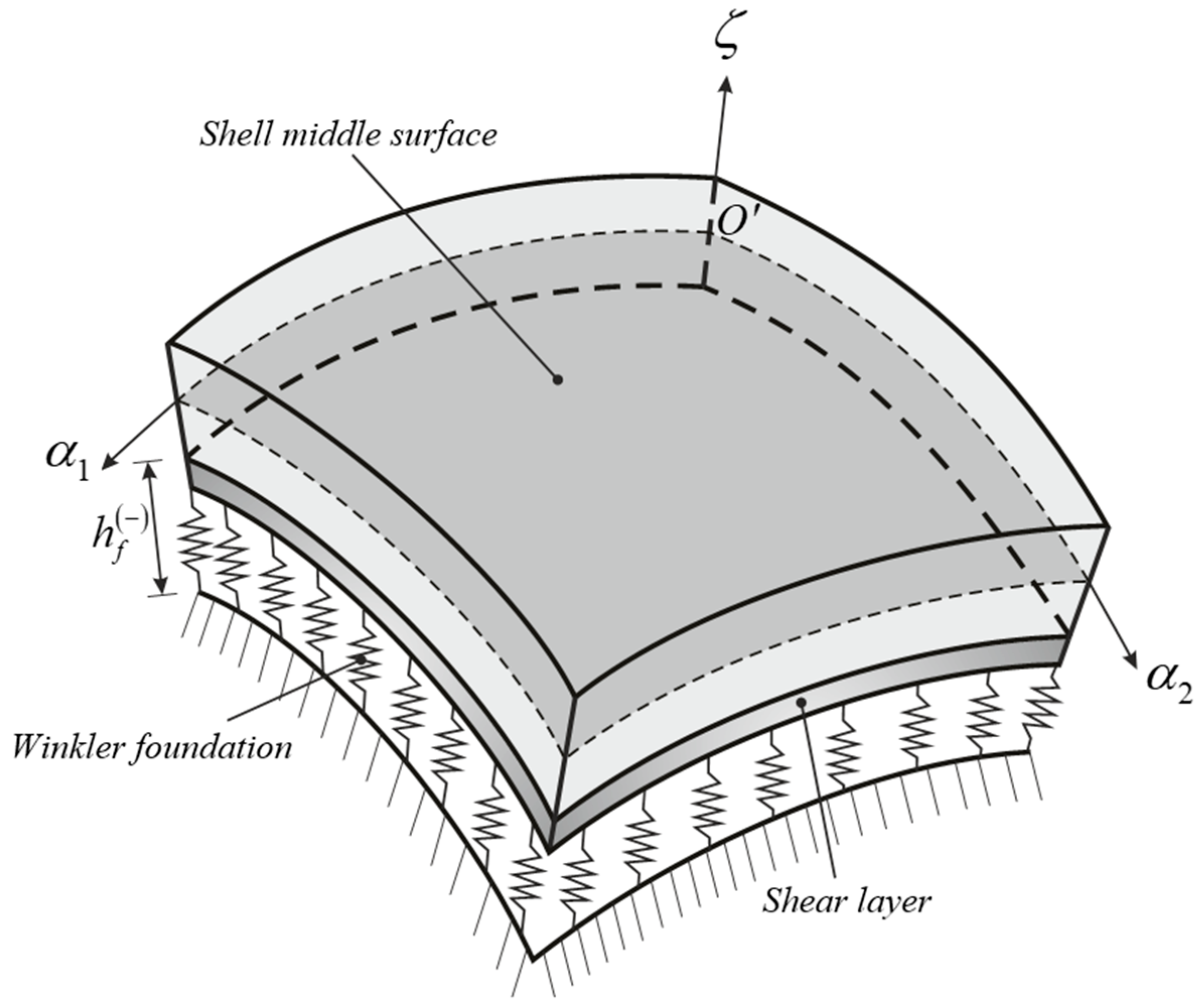
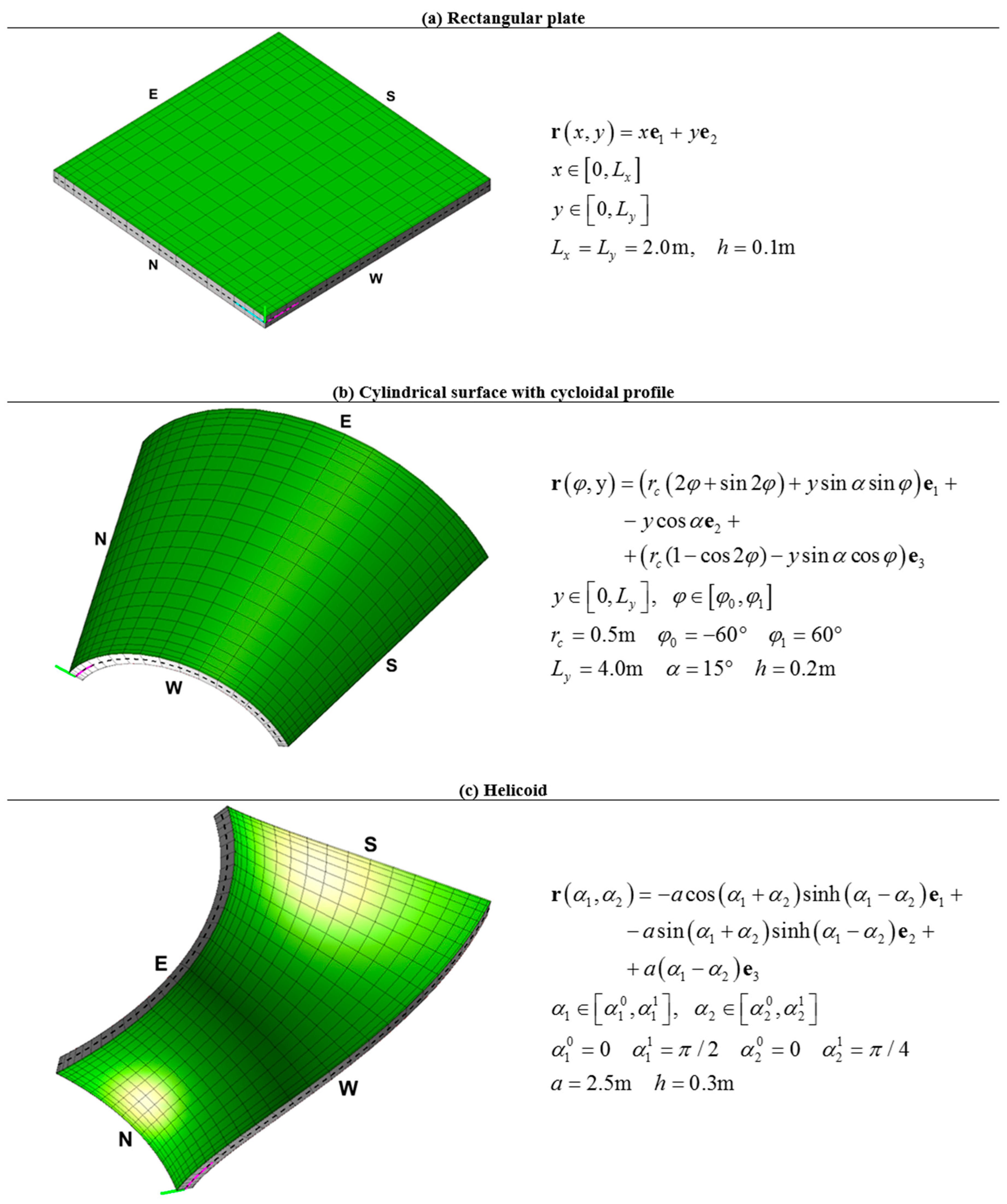
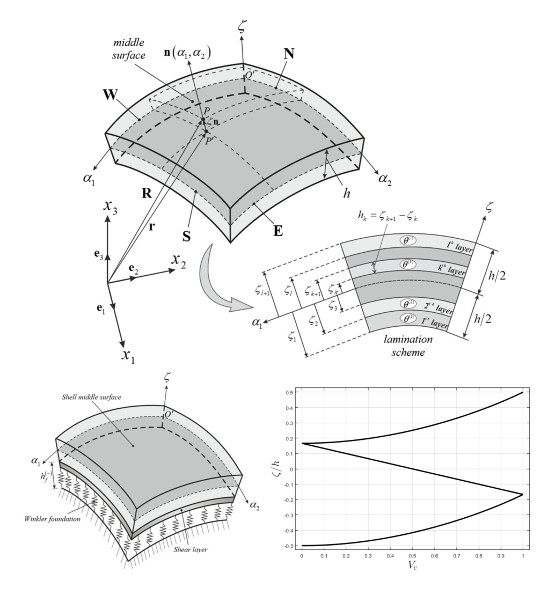
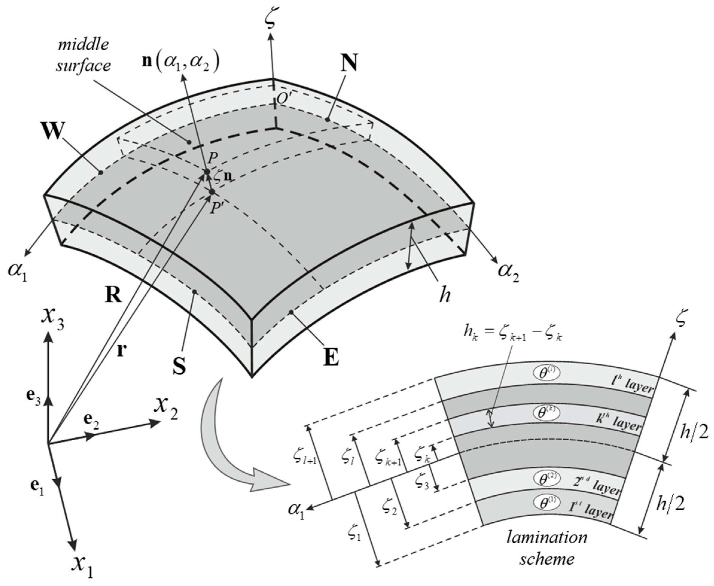
2.1. Geometry
2.2. Shell Formulation
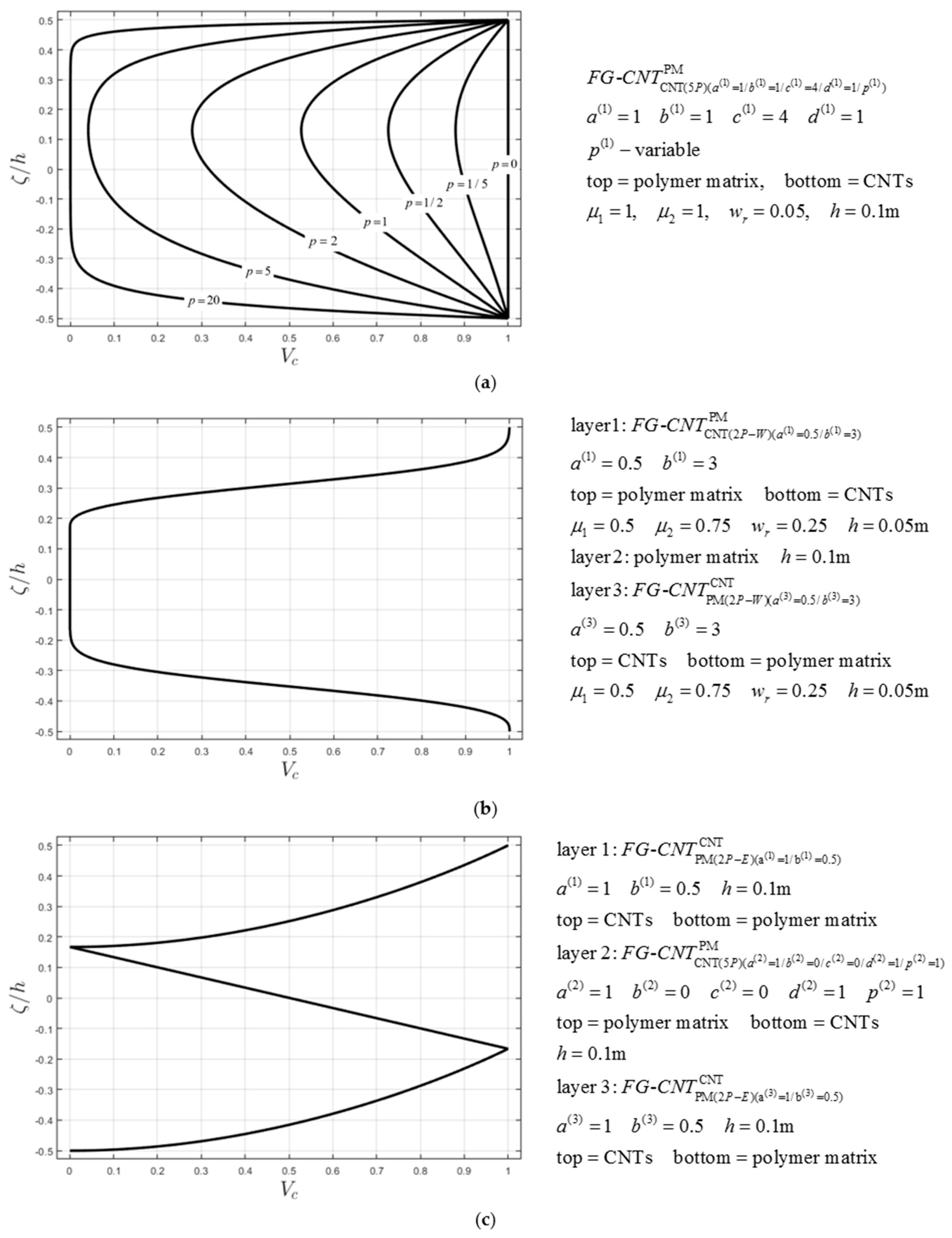
2.3. Functionally Graded Carbon Nanotube Reinforced Composite Structures
- Five-parameter exponential law
- Two-parameter exponential function
- Weibull function
- Five-parameter exponential law
- Two-parameter exponential function
- Weibull function
3. Numerical Scheme
4. Applications
4.1. Comparison with FEM
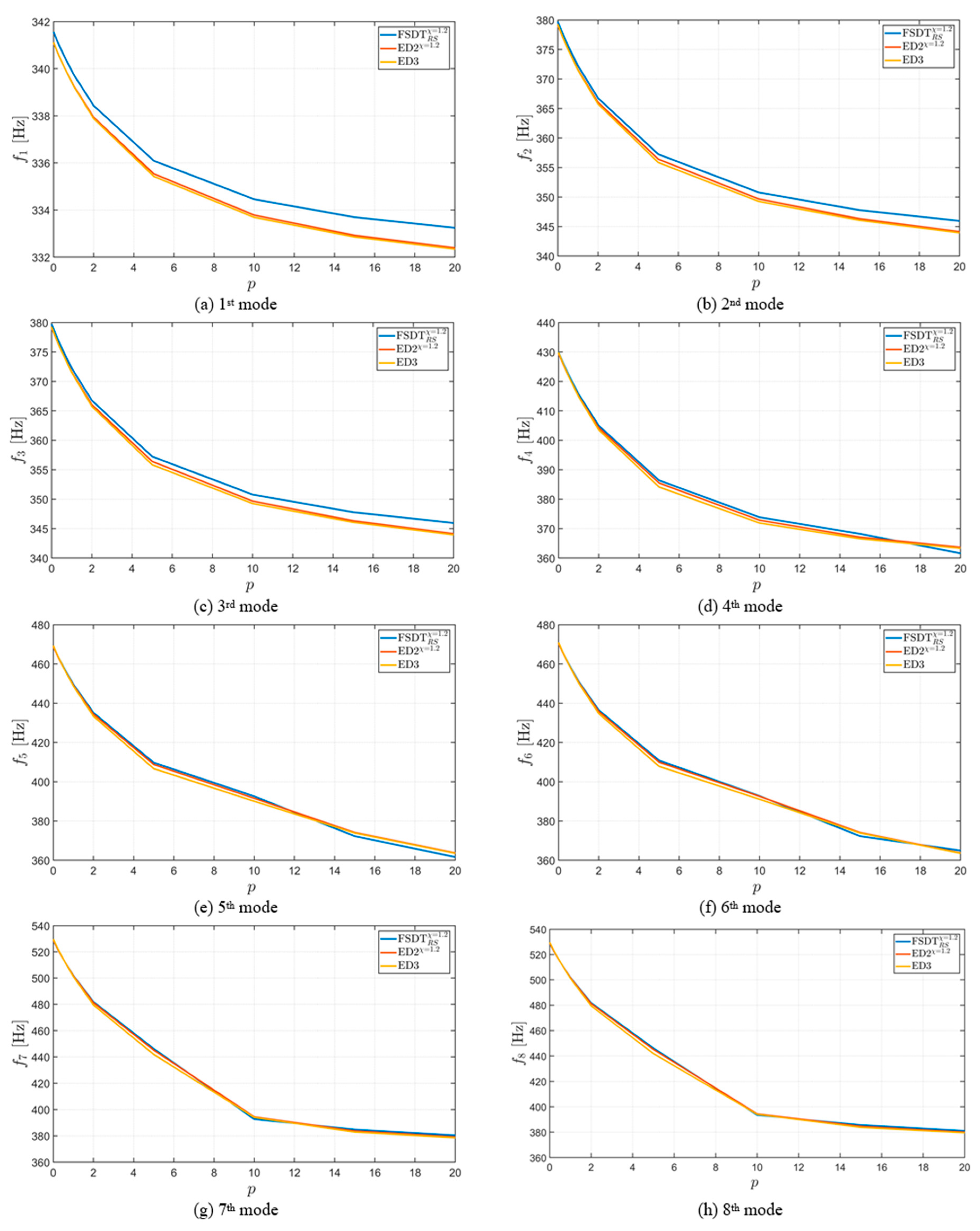
4.2. Effect of Through-the-Thickness Distribution of CNTs
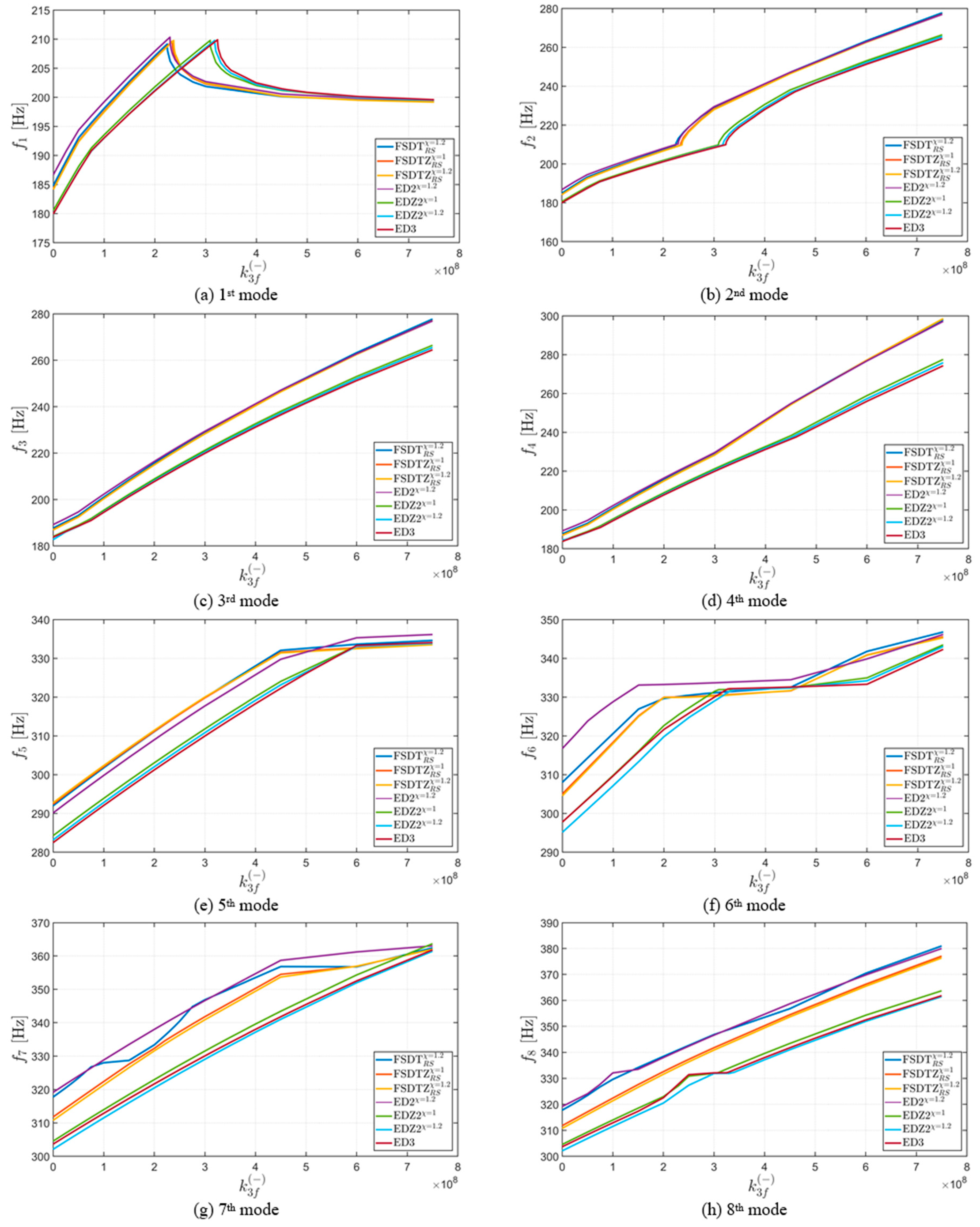
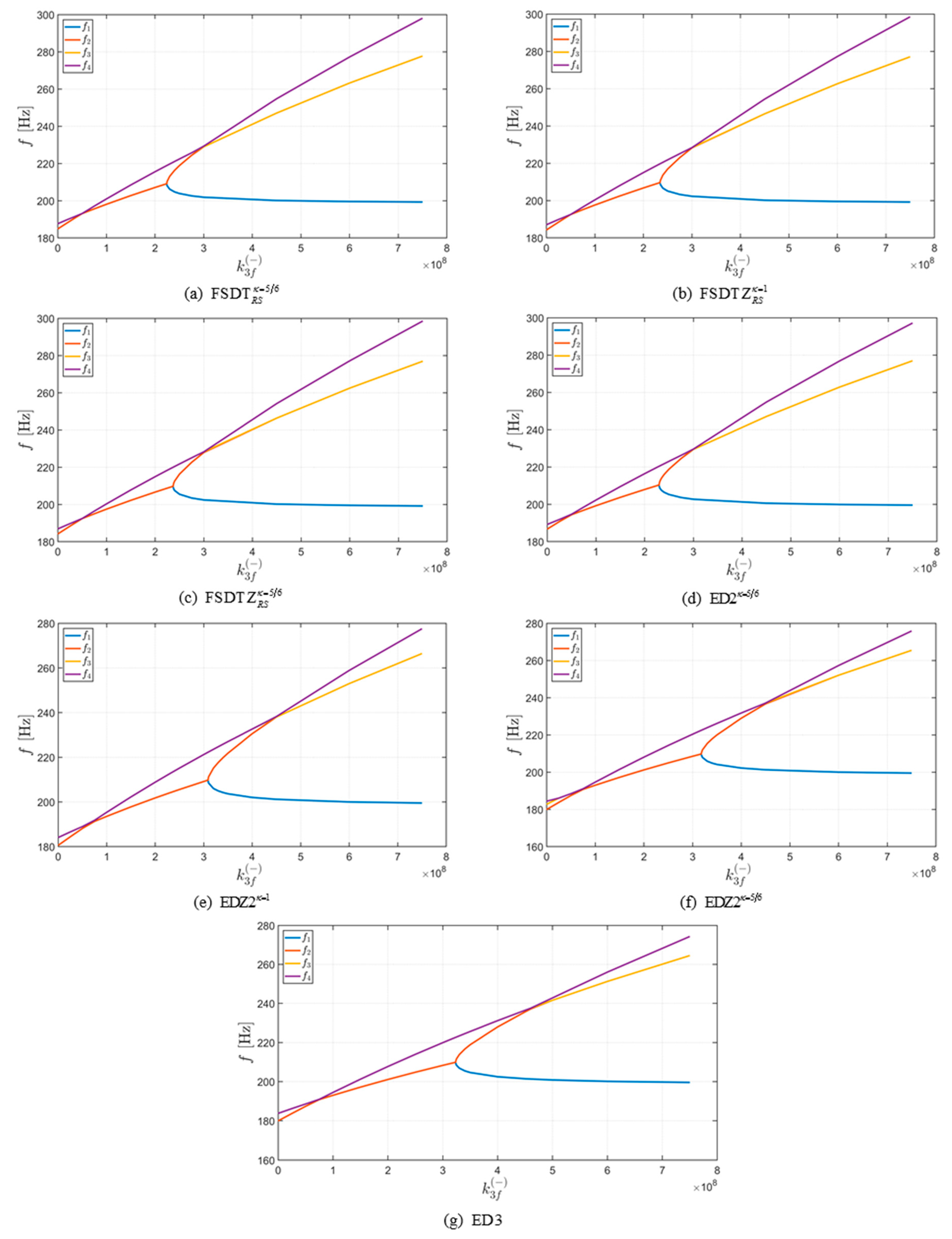
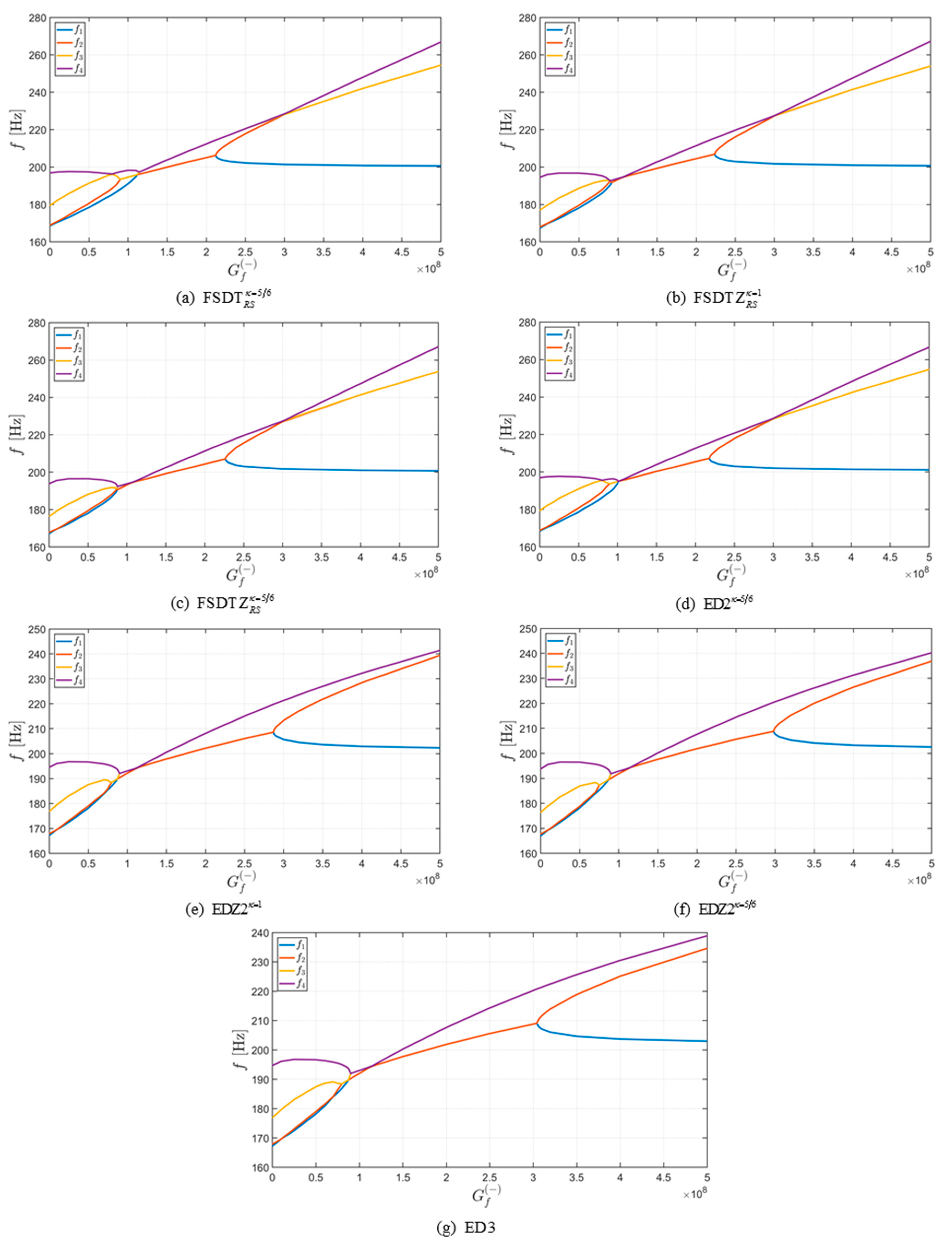
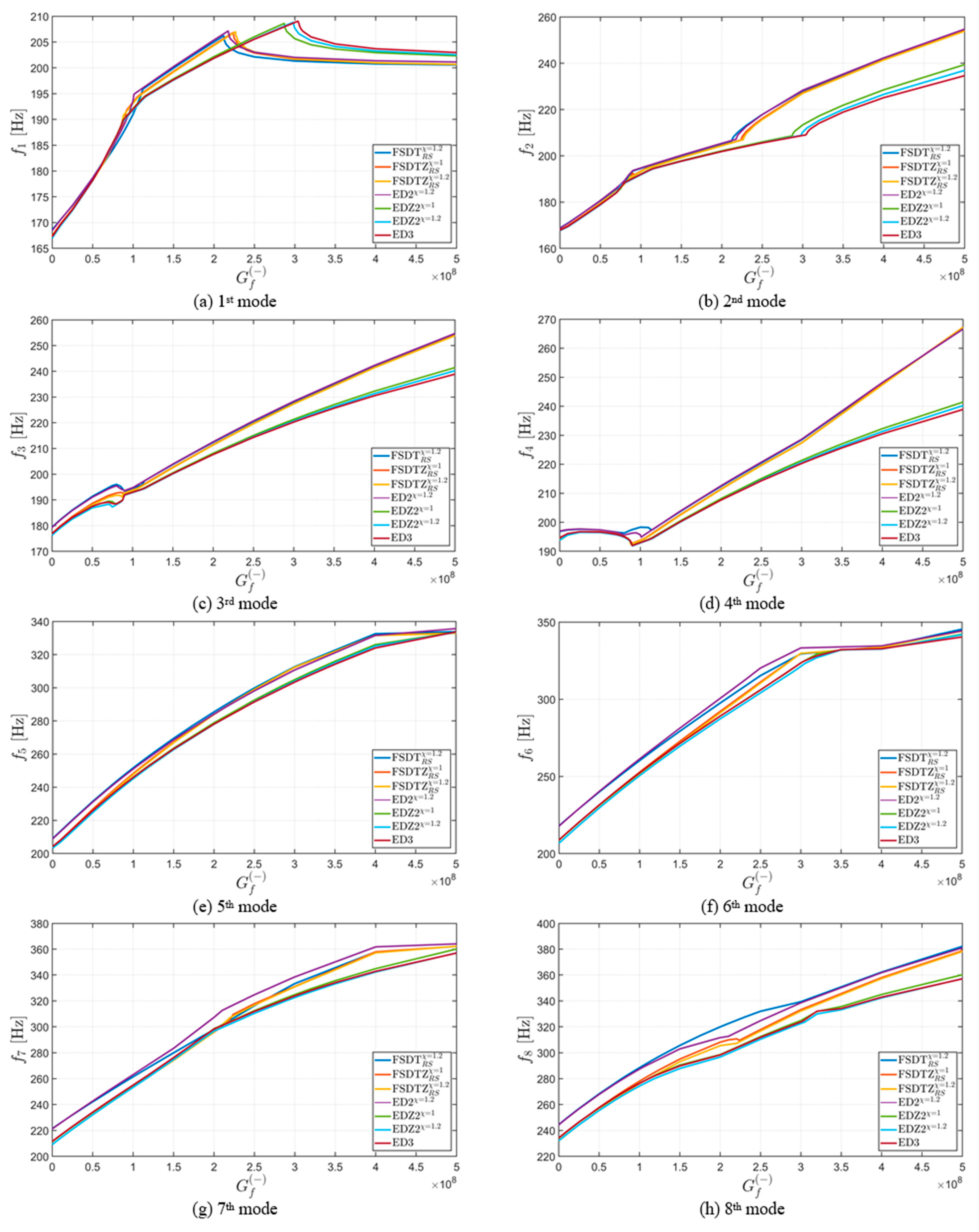
4.3. Effect of Elastic Foundation
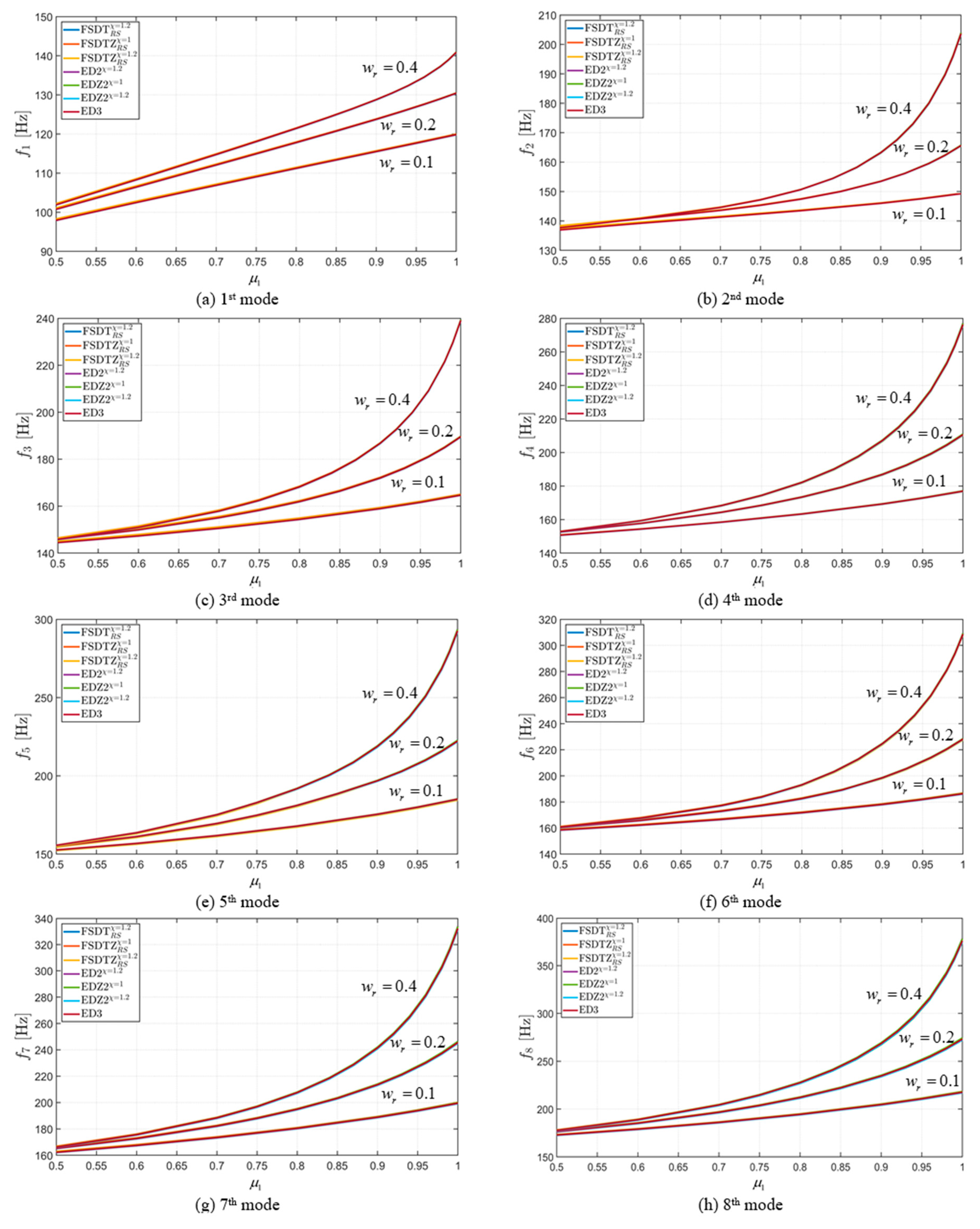
4.4. Effect of CNT Agglomeration
5. Conclusions
- -
- the choice and variation of the mechanical parameters that characterize the elastic foundation have a significant impact on the values of natural frequencies;
- -
- interesting behaviors can be observed in terms of natural frequencies when the mechanical parameters of the foundation are increased; in particular, bifurcation points and peculiar overlapping can be noted;
- -
- analogously, the natural frequency values are considerably affected by the agglomeration of CNTs; this aspect is extremely clear when the mass fraction of CNTs reaches higher values;
- -
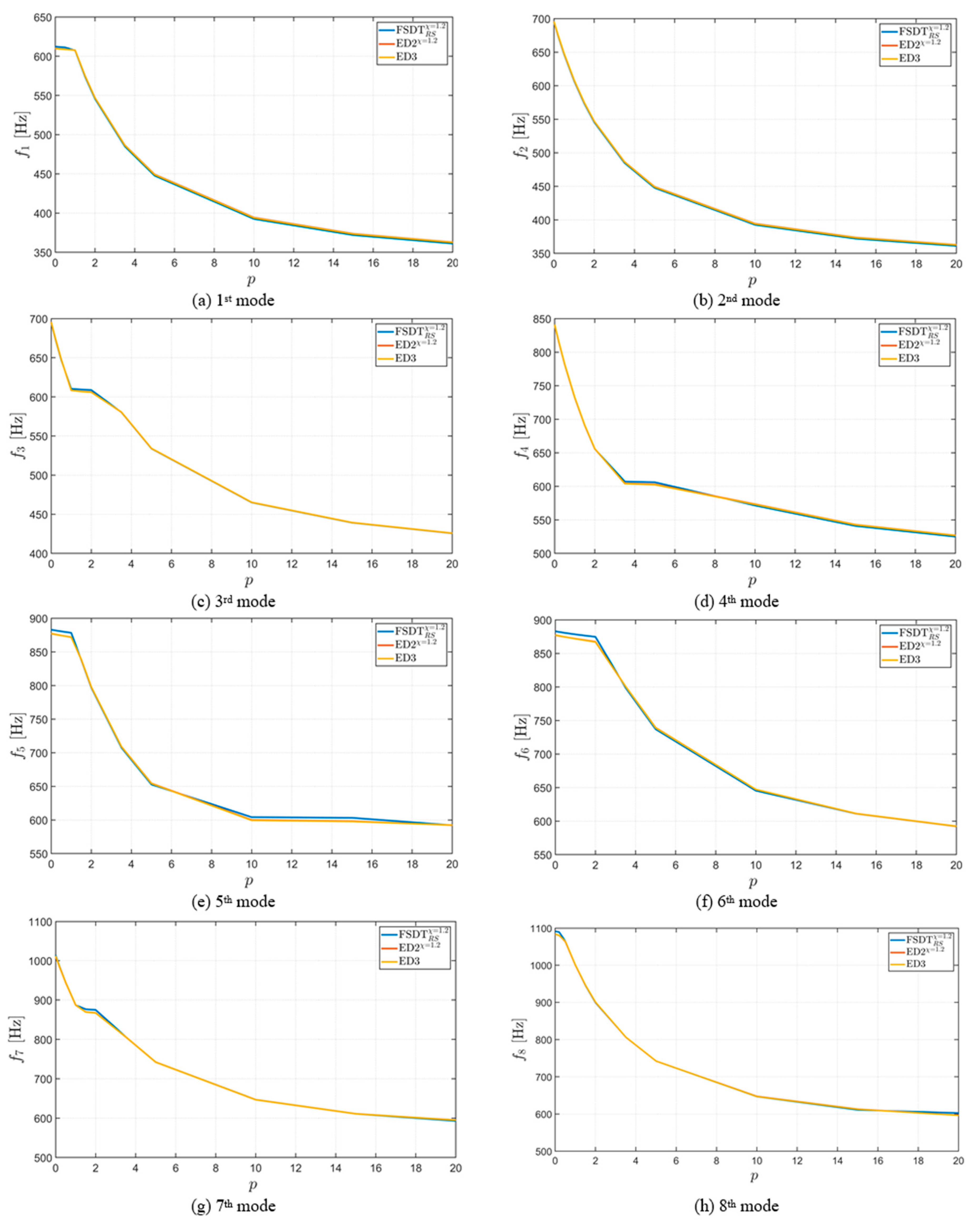
- the dynamic response of the structure can be modified by varying the parameters that define the through-the-thickness volume fraction distribution of CNTs;
- -
- several analytical distributions can be chosen to describe peculiar through-the-thickness volume fraction distributions, such as power law, exponential and Weibull functions; it should be noted that, at the present time, these distributions are not available in FEM commercial codes;
- -
- the comparison with the commercial FEM software shows good agreement of results, for those cases that can be analyzed and compared.
Acknowledgments
Author Contributions
Conflicts of Interest
References
- Iijima, S. Helical Microtubles of Graphitic Carbon. Nature 1991, 354, 56–58. [Google Scholar] [CrossRef]
- Iijima, S.; Ichihashi, T. Single-shell carbon nanotubes of 1-nm diameter. Nature 1993, 363, 603–605. [Google Scholar] [CrossRef]
- Popov, V.N.; Van Doren, V.E.; Balkanski, M. Elastic properties of crystals of single-walled carbon nanotubes. Solid State Commun. 2000, 114, 395–399. [Google Scholar] [CrossRef]
- Popov, V.N.; Van Doren, V.E. Elastic properties of single-walled carbon nanotubes. Phys. Rev. B 2000, 61, 3078–3084. [Google Scholar] [CrossRef]
- Qian, D.; Wagner, G.J.; Liu, W.K.; Yu, M.-F.; Ruoff, R.S. Mechanics of carbon nanotubes. Appl. Mech. Rev. 2002, 55, 495–533. [Google Scholar] [CrossRef]
- Thostenson, E.T.; Chou, T.-W. On the elastic properties of carbon nanotube-based composites: Modelling and characterization. J. Phys. D Appl. Phys. 2003, 36, 573–582. [Google Scholar] [CrossRef]
- Odegard, G.M.; Gates, T.S.; Wise, K.E.; Park, C.; Siochi, E.J. Constitutive modeling of nanotube-reinforced polymer composites. Compos. Sci. Technol. 2003, 63, 1671–1687. [Google Scholar] [CrossRef]
- Shen, L.; Li, J. Transversely isotropic elastic properties of single-walled carbon nanotubes. Phys. Rev. B 2004, 69, 1129–1133. [Google Scholar] [CrossRef]
- Ray, M.C.; Batra, R.C. Effective Properties of Carbon Nanotube and Piezoelectric Fiber Reinforced Hybrid Smart Composites. J. Appl. Mech. 2009, 76, 540–545. [Google Scholar] [CrossRef]
- Wang, J.F.; Liew, K.M. On the study of elastic properties of CNT-reinforced composites based on element-free MLS method with nanoscale cylindrical representative volume element. Compos. Struct. 2015, 124, 1–9. [Google Scholar] [CrossRef]
- Liew, K.M.; Lei, Z.X.; Zhang, L.W. Mechanical analysis of functionally graded carbon nanotube reinforced composites: A review. Compos. Struct. 2015, 120, 90–97. [Google Scholar] [CrossRef]
- Shen, H.-S. Nonlinear bending of functionally graded carbon nanotube-reinforced composite plates in thermal environments. Compos. Struct. 2009, 91, 9–19. [Google Scholar] [CrossRef]
- Raney, J.R.; Fraternali, F.; Amendola, A.; Daraio, C. Modeling and in situ identification of material parameters for layered structures based on carbon nanotube arrays. Compos. Struct. 2011, 93, 3013–3018. [Google Scholar] [CrossRef]
- Blesgen, T.; Fraternali, F.; Raney, J.R.; Amendola, A.; Daraio, C. Continuum limits of bistable spring models of carbon nanotube arrays accounting for material damage. Mech. Res. Commun. 2012, 45, 58–63. [Google Scholar] [CrossRef]
- Jam, J.E.; Pourasghar, A.; Kamarian, S. Effect of the Aspect Ratio and Waviness of Carbon Nanotubes on the Vibrational Behavior of Functionally Graded Nanocomposite Cylindrical Panels. Polym. Compos. 2012, 33, 2036–2044. [Google Scholar] [CrossRef]
- Alibeigloo, A.; Liew, K.M. Thermoelastic analysis of functionally graded carbon nanotube-reinforced composite plate using theory of elasticity. Compos. Struct. 2013, 106, 873–881. [Google Scholar] [CrossRef]
- Alibeigloo, A. Free vibration analysis of functionally graded carbon nanotube-reinforced composite cylindrical panel embedded in piezoelectric layers by using theory of elasticity. Eur. J. Mech. 2014, 44, 104–115. [Google Scholar] [CrossRef]
- Brischetto, S. A continuum elastic three-dimensional model for natural frequencies of single-walled carbon nanotubes. Compos. Part B Eng. 2014, 61, 222–228. [Google Scholar] [CrossRef]
- Brischetto, S. A continuum shell model including van der Waals interaction for free vibrations of double-walled carbon nanotubes. Comput. Model. Eng. Sci. 2015, 104, 305–327. [Google Scholar]
- Zhang, L.W.; Lei, Z.X.; Liew, K.M. Free vibration analysis of functionally graded carbon nanotube-reinforced composite triangular plates using the FSDT and element-free IMLS-Ritz method. Compos. Struct. 2015, 120, 189–199. [Google Scholar] [CrossRef]
- Zhang, L.W.; Lei, Z.X.; Liew, K.M. Vibration characteristic of moderately thick functionally graded carbon nanotube reinforced composite skew plates. Compos. Struct. 2015, 122, 172–183. [Google Scholar] [CrossRef]
- Lei, Z.X.; Zhang, L.W.; Liew, K.M. Free vibration analysis of laminated FG-CNT reinforced composite rectangular plates using the kp-Ritz method. Compos. Struct. 2015, 127, 245–259. [Google Scholar] [CrossRef]
- Mareishi, S.; Kalhori, H.; Rafiee, M.; Hosseini, S.M. Nonlinear forced vibration response of smart two-phase nano-composite beams to external harmonic excitations. Curved Layer. Struct. 2015, 2, 150–161. [Google Scholar] [CrossRef]
- Tornabene, F.; Fantuzzi, N.; Bacciocchi, M.; Viola, E. Effect of agglomeration on the natural frequencies of functionally graded carbon nanotube-reinforced laminated composite doubly-curved shells. Compos. Part B Eng. 2016, 89, 187–218. [Google Scholar] [CrossRef]
- Tornabene, F.; Fantuzzi, N.; Bacciocchi, M. Linear Static Response of Nanocomposite Plates and Shells Reinforced by Agglomerated Carbon Nanotubes. Compos. Part B Eng. 2017, 115, 449–476. [Google Scholar] [CrossRef]
- Fantuzzi, N.; Tornabene, F.; Bacciocchi, M.; Dimitri, R. Free vibration analysis of arbitrarily shaped Functionally Graded Carbon Nanotube-reinforced plates. Compos. Part B Eng. 2017, 115, 384–408. [Google Scholar] [CrossRef]
- Tornabene, F.; Bacciocchi, M.; Fantuzzi, N.; Reddy, J.N. Multiscale approach for three-phase CNT/polymer/fiber laminated nanocomposite structures. Polym. Compos. 2017. [Google Scholar] [CrossRef]
- Akgöz, B.; Civalek, Ö. A size-dependent beam model for stability of axially loaded carbon nanotubes surrounded by Pasternak elastic foundation. Compos. Struct. 2017, 176, 1028–1038. [Google Scholar] [CrossRef]
- Civalek, Ö. Free vibration of carbon nanotubes reinforced (CNTR) and functionally graded shells and plates based on FSDT via discrete singular convolution method. Compos. Part B Eng. 2017, 111, 45–59. [Google Scholar] [CrossRef]
- Chamis, C.C. Failure Criteria for Filamentary Composites; TN D-5367; NASA: Washington, DC, USA, 1969.
- Chamis, C.C. Thermoelastic Properties of Unidirectional Filamentary Composites by a Semiempirical Micromechanics Theory; Union Carbide Corp Cleveland Ohio Carbon Products Div: Cleveland, OH, USA, 1974. [Google Scholar]
- Shi, D.-L.; Huang, Y.Y.; Hwang, K.-C.; Gao, H. The Effect of Nanotube Waviness and Agglomeration on the Elastic Property of Carbon Nanotube-Reinforced Composites. J. Eng. Mater. Technol. 2004, 126, 250–257. [Google Scholar] [CrossRef]
- Mori, T.; Tanaka, K. Average stress in matrix and average elastic energy of materials with Misfitting inclusions. Acta Metall. 1973, 21, 571–574. [Google Scholar] [CrossRef]
- Hill, R. Theory of Mechanical Properties of Fibre-Strengthened Materials: I. Elastic Behavior. J. Mech. Phys. Solids 1964, 12, 199–212. [Google Scholar] [CrossRef]
- Hill, R. Theory of Mechanical Properties of Fibre-Strengthened Materials: II. Inelastic Behavior. J. Mech. Phys. Solids 1964, 12, 213–218. [Google Scholar] [CrossRef]
- Hedayati, H.; Sobhani Aragh, B. Influence of graded agglomerated CNTs on vibration of CNT-reinforced annular sectorial plates resing on Pasternak foundation. Appl. Math. Comput. 2012, 218, 8715–8735. [Google Scholar]
- Aragh, B.S.; Barati, A.H.N.; Hedayati, H. Eshelby-Mori-Tanaka approach for vibrational behavior of continuously graded carbon nanotube-reinforced cylindrical panels. Compos. Part B Eng. 2012, 43, 1943–1954. [Google Scholar] [CrossRef]
- Aragh, B.S.; Farahani, E.B.; Barati, A.H.N. Natural frequency analysis of continuously graded carbon nanotube-reinforced cylindrical shells based on third-order shear deformation theory. Math. Mech. Solids 2013, 18, 264–284. [Google Scholar] [CrossRef]
- Reddy, J.N. A Simple Higher-Order Theory for Laminated Composite Plates. J. Appl. Mech. 1984, 51, 745–752. [Google Scholar] [CrossRef]
- Bert, C.W. A Critical Evaluation of New Plate Theories Applied to Laminated Composites. Compos. Struct. 1984, 2, 329–347. [Google Scholar] [CrossRef]
- Reddy, J.N.; Liu, C.F. A higher-order shear deformation theory for laminated elastic shells. Int. J. Eng. Sci. 1985, 23, 319–330. [Google Scholar] [CrossRef]
- Reddy, J.N. A Generalization of the Two-Dimensional Theories of Laminated Composite Plates. Commun. Appl. Numer. Methods Biomed. Eng. 1987, 3, 173–180. [Google Scholar] [CrossRef]
- Librescu, L.; Reddy, J.N. A few remarks concerning several refined theories of anisotropic composite laminated plates. Int. J. Eng. Sci. 1989, 27, 515–527. [Google Scholar] [CrossRef]
- Reddy, J.N. On Refined Theories of Composite Laminates. Meccanica 1990, 25, 230–238. [Google Scholar] [CrossRef]
- Robbins, D.H.; Reddy, J.N. Modeling of Thick Composites Using a Layer-Wise Laminate Theory. Int. J. Numer. Methods Eng. 1993, 36, 655–677. [Google Scholar] [CrossRef]
- Reddy, J.N. Mechanics of Laminated Composite Plates and Shells; CRC Press: Boca Raton, FL, USA, 2004. [Google Scholar]
- Alibeigloo, A.; Shakeri, M.; Kari, M.R. Free vibration analysis of antisymmetric laminated rectangular plates with distributed patch mass using third-order shear deformation theory. Ocean Eng. 2008, 35, 183–190. [Google Scholar] [CrossRef]
- Demasi, L. ∞3 Hierarchy plate theories for thick and thin composite plates: The generalized unified formulation. Compos. Struct. 2008, 84, 256–270. [Google Scholar] [CrossRef]
- Amabili, M.; Reddy, J.N. A new non-linear higher-order shear deformation theory for large-amplitude vibrations of laminated doubly curved shells. Int. J. Nonlinear Mech. 2010, 45, 409–418. [Google Scholar] [CrossRef]
- Mantari, J.L.; Oktem, A.S.; Soares, C.G. A new trigonometric layerwise shear deformation theory for the finite element analysis of laminated composite and sandwich plates. Comput. Struct. 2012, 94–95, 45–53. [Google Scholar] [CrossRef]
- Mantari, J.L.; Soares, C.G. Generalized layerwise HSDT and finite element formulation for symmetric laminated and sandwich composite plates. Compos. Struct. 2013, 105, 319–331. [Google Scholar] [CrossRef]
- Vo, T.P.; Thai, H.-T.; Nguyen, T.-K.; Lanc, D.; Karamanli, A. Flexural analysis of laminated composite and sandwich beams using a four-unknown shear and normal deformation theory. Compos. Struct. 2017, 176, 388–397. [Google Scholar] [CrossRef]
- D’Ottavio, M. A Sublaminate Generalized Unified Formulation for the analysis of composite structures. Compos. Struct. 2016, 142, 187–199. [Google Scholar] [CrossRef]
- D’Ottavio, M.; Dozio, L.; Vescovini, R.; Polit, O. Bending analysis of composite laminated and sandwich structures using sublaminate variable-kinematic Ritz models. Compos. Struct. 2016, 155, 45–62. [Google Scholar] [CrossRef]
- Tornabene, F.; Fantuzzi, N.; Bacciocchi, M.; Reddy, J.N. An Equivalent Layer-Wise Approach for the Free Vibration Analysis of Thick and Thin Laminated Sandwich Shells. Appl. Sci. 2017, 7, 1–34. [Google Scholar] [CrossRef]
- Tornabene, F.; Fantuzzi, N.; Bacciocchi, M. Linear Static Behavior of Damaged Laminated Composite Plates and Shells. Materials 2017, 10, 1–52. [Google Scholar] [CrossRef] [PubMed]
- Reddy, J.N.; Chin, C.D. Thermomechanical Analysis of Functionally Graded Cylinders and Plates. J. Therm. Stress. 1998, 21, 593–626. [Google Scholar] [CrossRef]
- Loy, C.T.; Lam, K.Y.; Reddy, J.N. Vibration of functionally graded cylindrical shells. Int. J. Mech. Sci. 1999, 41, 309–324. [Google Scholar] [CrossRef]
- Pradhan, S.C.; Loy, C.T.; Lam, K.Y.; Reddy, J.N. Vibration characteristics of functionally graded cylindrical shells under various boundary conditions. Appl. Acoust. 2000, 61, 111–129. [Google Scholar] [CrossRef]
- Reddy, J.N. Analysis of functionally graded plates. Int. J. Numer. Methods Eng. 2000, 47, 663–684. [Google Scholar] [CrossRef]
- Arshad, S.H.; Naeem, M.N.; Sultana, N. Frequency analysis of functionally graded material cylindrical shells with various volume fractions laws. J. Mech. Eng. Sci. 2007, 221, 1483–1495. [Google Scholar] [CrossRef]
- Amabili, M. Nonlinear Vibrations and Stability of Shells and Plates; Cambridge University Press: New York, NY, USA, 2008. [Google Scholar]
- Reddy, J.N. Microstructure-dependent couple stress theories of functionally graded beams. J. Mech. Phys. Solids 2011, 59, 2382–2399. [Google Scholar] [CrossRef]
- Reddy, J.N.; Kim, J. A nonlinear modified couple stress-based third-order theory of functionally graded plates. Compos. Struct. 2012, 94, 1128–1143. [Google Scholar] [CrossRef]
- Strozzi, M.; Pellicano, F. Nonlinear vibrations of functionally graded cylindrical shells. Thin-Walled Struct. 2013, 67, 63–77. [Google Scholar] [CrossRef]
- Kim, J.; Reddy, J.N. A general third-order theory of functionally graded plates with modified couple stress effect and the von Kármán nonlinearity: Theory and finite element analysis. Acta Mech. 2015, 226, 2973–2998. [Google Scholar] [CrossRef]
- Sofiyev, A.H.; Kuruoglu, N. Dynamic instability of three-layered cylindrical shells containing an FGM interlayer. Thin-Walled Struct. 2015, 93, 10–21. [Google Scholar] [CrossRef]
- Sofiyev, A.H.; Kuruoglu, N. Domains of dynamic instability of FGM conical shells under time dependent periodic loads. Compos. Struct. 2016, 136, 139–148. [Google Scholar] [CrossRef]
- Rivera, M.G.; Reddy, J.N. Stress analysis of functionally graded shells using a 7-parameter shell element. Mech. Res. Commun. 2016, 78, 60–70. [Google Scholar] [CrossRef]
- Tornabene, F.; Viola, E. Free Vibration Analysis of Functionally Graded Panels and Shells of Revolution. Meccanica 2009, 44, 255–281. [Google Scholar] [CrossRef]
- Viola, E.; Tornabene, F. Free Vibrations of Three Parameter Functionally Graded Parabolic Panels of Revolution. Mech. Res. Commun. 2009, 36, 587–594. [Google Scholar] [CrossRef]
- Tornabene, F. Free Vibration Analysis of Functionally Graded Conical, Cylindrical Shell and Annular Plate Structures with a Four-parameter Power-Law Distribution. Comput. Methods Appl. Mech. Eng. 2009, 198, 2911–2935. [Google Scholar] [CrossRef]
- Akgöz, B.; Civalek, Ö. Bending analysis of FG microbeams resting on Winkler elastic foundation via strain gradient elasticity. Compos. Struct. 2015, 134, 294–301. [Google Scholar] [CrossRef]
- Lanc, D.; Vo, T.P.; Turkalj, G.; Lee, J. Buckling analysis of thin-walled functionally graded sandwich box beams. Thin-Walled Struct. 2015, 86, 148–156. [Google Scholar] [CrossRef]
- Tornabene, F.; Fantuzzi, N.; Viola, E.; Batra, R.C. Stress and strain recovery for functionally graded free-form and doubly-curved sandwich shells using higher-order equivalent single layer theory. Compos. Struct. 2015, 119, 67–89. [Google Scholar] [CrossRef]
- Lanc, D.; Turkalj, G.; Vo, T.P.; Brnić, J. Nonlinear buckling behaviours of thin-walled functionally graded open section beams. Compos. Struct. 2016, 152, 829–839. [Google Scholar] [CrossRef]
- Fazzolari, F.A. Reissner’s Mixed Variational Theorem and Variable Kinematics in the Modelling of Laminated Composite and FGM Doubly-Curved Shells. Compos. Part B Eng. 2016, 89, 408–423. [Google Scholar] [CrossRef]
- Fazzolari, F.A. Stability Analysis of FGM Sandwich Plates by Using Variable-kinematics Ritz Models. Mech. Adv. Mater. Struct. 2016, 23, 1104–1113. [Google Scholar] [CrossRef]
- Tornabene, F.; Brischetto, S.; Fantuzzi, N.; Bacciocchi, M. Boundary Conditions in 2D Numerical and 3D Exact Models for Cylindrical Bending Analysis of Functionally Graded Structures. Shock Vib. 2016, 2016, 1–17. [Google Scholar] [CrossRef]
- Brischetto, S.; Tornabene, F.; Fantuzzi, N.; Viola, E. 3D Exact and 2D Generalized Differential Quadrature Models for Free Vibration Analysis of Functionally Graded Plates and Cylinders. Meccanica 2016, 51, 2059–2098. [Google Scholar] [CrossRef]
- Fantuzzi, N.; Brischetto, S.; Tornabene, F.; Viola, E. 2D and 3D Shell Models for the Free Vibration Investigation of Functionally Graded Cylindrical and Spherical Panels. Compos. Struct. 2016, 154, 573–590. [Google Scholar] [CrossRef]
- Civalek, Ö. Vibration of laminated composite panels and curved plates with different types of FGM composite constituent. Compos. Part B Eng. 2017, 122, 89–108. [Google Scholar] [CrossRef]
- Tornabene, F.; Fantuzzi, N.; Bacciocchi, M.; Viola, E.; Reddy, J.N. A Numerical Investigation on the Natural Frequencies of FGM Sandwich Shells with Variable Thickness by the Local Generalized Differential Quadrature Method. Appl. Sci. 2017, 7, 1–39. [Google Scholar] [CrossRef]
- Barretta, R.; Feo, L.; Luciano, R. Some closed-form solutions of functionally graded beams undergoing nonuniform torsion. Compos. Struct. 2015, 123, 132–136. [Google Scholar] [CrossRef]
- Barretta, R.; Brčić, M.; Čanađija, M.; Luciano, R.; Marotti de Sciarra, F. Application of gradient elasticity to armchair carbon nanotubes: Size effects and constitutive parameters assessment. Eur. J. Mech. A Solids 2017, 65, 1–13. [Google Scholar] [CrossRef]
- Romano, G.; Barretta, R. Nonlocal elasticity in nanobeams: The stress-driven integral model. Int. J. Eng. Sci. 2017, 115, 14–27. [Google Scholar] [CrossRef]
- Romano, G.; Barretta, R.; Diaco, M. On nonlocal integral models for elastic nano-beams. Int. J. Mech. Sci. 2017, 131–132, 490–499. [Google Scholar] [CrossRef]
- Marotti de Sciarra, F.; Barretta, R. A new nonlocal bending model for Euler-Bernoulli nanobeams. Mech. Res. Commun. 2014, 62, 25–30. [Google Scholar] [CrossRef]
- Apuzzo, A.; Barretta, R.; Luciano, R.; Marotti de Sciarra, F.; Penna, R. Free vibrations of Bernoulli-Euler nano-beams by the stress-driven nonlocal integral model. Compos. Part B Eng. 2017, 123, 105–111. [Google Scholar] [CrossRef]
- Barretta, R. Analogies between Kirchhoff plates and Saint-Venant beams under flexure. Acta Mech. 2014, 225, 2075–2083. [Google Scholar] [CrossRef]
- Barretta, R. On the relative position of twist and shear centres in the orthotropic and fiberwise homogeneous Saint–Venant beam theory. Int. J. Solids Struct. 2012, 49, 3038–3046. [Google Scholar] [CrossRef]
- Barretta, R. Analogies between Kirchhoff plates and Saint-Venant beams under torsion. Acta Mech. 2013, 224, 2955–2964. [Google Scholar] [CrossRef]
- Barretta, R. On Cesàro-Volterra Method in Orthotropic Saint-Venant Beam. J. Elast. 2013, 112, 233–253. [Google Scholar] [CrossRef]
- Carrera, E. A refined multi-layered finite-element model applied to linear and non-linear analysis of sandwich plates. Compos. Sci. Technol. 1998, 58, 1553–1569. [Google Scholar] [CrossRef]
- Carrera, E. Theories and Finite Elements for Multilayered, Anisotropic, Composite Plates and Shells. Arch. Comput. Methods Eng. 2002, 9, 87–140. [Google Scholar] [CrossRef]
- Carrera, E. Theories and Finite Elements for Multilayered Plates and Shells: A Unified Compact Formulation with Numerical Assessment and Benchmarking. Arch. Comput. Methods Eng. 2003, 10, 215–296. [Google Scholar] [CrossRef]
- Carrera, E. Historical review of zig-zag theories for multilayered plates and shells. Appl. Mech. Rev. 2003, 56, 287–308. [Google Scholar] [CrossRef]
- Carrera, E. On the use of the Murakami’s zig-zag function in the modeling of layered plates and shells. Comput. Struct. 2004, 82, 541–554. [Google Scholar] [CrossRef]
- Tornabene, F.; Fantuzzi, N.; Bacciocchi, M.; Viola, E. Laminated Composite Doubly-Curved Shell Structures. Differential Geometry. Higher-Order Structural Theories; Esculapio: Bologna, Italy, 2016. [Google Scholar]
- Tornabene, F.; Fantuzzi, N.; Bacciocchi, M.; Viola, E. Laminated Composite Doubly-Curved Shell Structures. Differential and Integral Quadrature. Strong Formulation Finite Element Method; Esculapio: Bologna, Italy, 2016. [Google Scholar]
- Tornabene, F.; Viola, E.; Fantuzzi, N. General higher-order equivalent single layer theory for free vibrations of doubly-curved laminated composite shells and panels. Compos. Struct. 2013, 104, 94–117. [Google Scholar] [CrossRef]
- Tornabene, F.; Fantuzzi, N.; Viola, E.; Carrera, E. Static Analysis of Doubly-Curved Anisotropic Shells and Panels Using CUF Approach, Differential Geometry and Differential Quadrature Method. Compos. Struct. 2014, 107, 675–697. [Google Scholar] [CrossRef]
- Tornabene, F.; Fantuzzi, N.; Bacciocchi, M. The Local GDQ Method for the Natural Frequencies of Doubly-Curved Shells with Variable Thickness: A General Formulation. Compos. Part B Eng. 2016, 92, 265–289. [Google Scholar] [CrossRef]
- Tornabene, F.; Fantuzzi, N.; Viola, E. Inter-Laminar Stress Recovery Procedure for Doubly-Curved, Singly-Curved, Revolution Shells with Variable Radii of Curvature and Plates Using Generalized Higher-Order Theories and the Local GDQ Method. Mech. Adv. Mater. Struct. 2016, 23, 1019–1045. [Google Scholar] [CrossRef]
- Tornabene, F.; Fantuzzi, N.; Bacciocchi, M. The GDQ Method for the Free Vibration Analysis of Arbitrarily Shaped Laminated Composite Shells Using a NURBS-Based Isogeometric Approach. Compos. Struct. 2016, 154, 190–218. [Google Scholar] [CrossRef]
- Bacciocchi, M.; Eisenberger, M.; Fantuzzi, N.; Tornabene, F.; Viola, E. Vibration Analysis of Variable Thickness Plates and Shells by the Generalized Differential Quadrature Method. Compos. Struct. 2016, 156, 218–237. [Google Scholar] [CrossRef]
- Tornabene, F.; Fantuzzi, N.; Bacciocchi, M. On the Mechanics of Laminated Doubly-Curved Shells Subjected to Point and Line Loads. Int. J. Eng. Sci. 2016, 109, 115–164. [Google Scholar] [CrossRef]
- Tornabene, F.; Fantuzzi, N.; Bacciocchi, M. A New Doubly-Curved Shell Element for the Free Vibrations of Arbitrarily Shaped Laminated Structures Based on Weak Formulation IsoGeometric Analysis. Compos. Struct. 2017, 171, 429–461. [Google Scholar] [CrossRef]
- Tornabene, F.; Fantuzzi, N.; Bacciocchi, M. Foam core composite sandwich plates and shells with variable stiffness: Effect of the curvilinear fiber path on the modal response. J. Sandw. Struct. Mater. 2017. [Google Scholar] [CrossRef]
- Tornabene, F.; Fantuzzi, N.; Bacciocchi, M. Refined Shear Deformation Theories for Laminated Composite Arches and Beams with Variable Thickness: Natural Frequency Analysis. Eng. Anal. Bound. Elem. 2017. [Google Scholar] [CrossRef]
- Cheung, Y.K.; Zienkiewicz, O.C. Plates and tanks on elastic foundations—An application of finite element method. Int. J. Solids Struct. 1965, 1, 451–461. [Google Scholar] [CrossRef]
- Bezine, G. A new boundary element method for bending of plates on elastic foundation. Int. J. Solids Struct. 1988, 24, 557–565. [Google Scholar] [CrossRef]
- Katsikadelis, J.T. Large deflection analysis of plates on elastic foundation by the boundary element method. Int. J. Solids Struct. 1991, 27, 1867–1878. [Google Scholar] [CrossRef]
- Qin, Q.H.; Diao, S. Nonlinear analysis of thick plates on an elastic foundation by HT FE with p-extension capabilities. Int. J. Solids Struct. 1996, 33, 4583–4604. [Google Scholar] [CrossRef]
- Akbarov, S.D.; Kocatürk, T. On the bending problems of anisotropic (orthotropic) plates resting on elastic foundations that react in compression only. Int. J. Solids Struct. 1997, 34, 3673–3689. [Google Scholar] [CrossRef]
- Shen, H.-S.; Li, Q.S. Postbuckling of shear deformable laminated plates resting on a tensionless elastic foundation subjected to mechanical or thermal loading. Int. J. Solids Struct. 2004, 41, 4769–4785. [Google Scholar] [CrossRef]
- Civalek, O. Geometrically nonlinear dynamic analysis of doubly curved isotropic shells resting on elastic foundation by a combination of harmonic differential quadrature-finite difference methods. Int. J. Press. Vessels Pip. 2005, 82, 753–761. [Google Scholar] [CrossRef]
- Avramidis, I.E.; Morfidis, K. Bending of beams on three-parameter elastic foundation. Int. J. Solids Struct. 2006, 43, 357–375. [Google Scholar] [CrossRef]
- Golovko, G.B.; Lugovoi, P.Z.; Meish, V.F. Solution of axisymmetric dynamic problems for cylindrical shells on an elastic foundation. Int. Appl. Mech. 2007, 43, 785–793. [Google Scholar] [CrossRef]
- Malekzadeh, P.; Farid, M. A DQ large deformation analysis of composite plates on nonlinear elastic foundations. Compos. Struct. 2007, 79, 251–260. [Google Scholar] [CrossRef]
- Malekzadeh, P.; Setoodeh, A.R. Large deformation analysis of moderately thick laminated plates on nonlinear elastic foundations by DQM. Compos. Struct. 2007, 80, 569–579. [Google Scholar] [CrossRef]
- Sofiyev, A.H. Buckling analysis of FGM circular shells under combined loads and resting on Pasternak type elastic foundations. Mech. Res. Commun. 2010, 37, 539–544. [Google Scholar] [CrossRef]
- Wang, J.; Zhang, C. A three-parameter elastic foundation model for interface stresses in curved beams externally strengthened by a thin FRP plate. Int. J. Solids Struct. 2010, 47, 998–1006. [Google Scholar] [CrossRef]
- Sofiyev, A.H.; Kuruoglu, N. Natural frequency of laminated orthotropic shells with different boundary conditions and resting on the Pasternak type elastic foundation. Compos. Part B Eng. 2011, 42, 1562–1570. [Google Scholar] [CrossRef]
- Thai, H.-T.; Choi, D.-H. A refined shear deformation theory for free vibration of functionally graded plates on elastic foundation. Compos. Part B Eng. 2012, 43, 2335–2347. [Google Scholar] [CrossRef]
- Tornabene, F.; Ceruti, A. Free-form Laminated Doubly-Curved Shells and Panels of Revolution on Winkler-Pasternak Elastic Foundations: A 2D GDQ Solution for Static and Free Vibration Analysis. World J. Mech. 2013, 3, 1–25. [Google Scholar] [CrossRef]
- Tornabene, F.; Reddy, J.N. FGM and Laminated Doubly-Curved and degenerate Shells resting on Nonlinear Elastic Foundation: A GDQ Solution for Static Analysis with a Posteriori Stress and strain Recovery. J. Indian Inst. Sci. 2013, 93, 635–688. [Google Scholar]
- Tornabene, F.; Fantuzzi, N.; Viola, E.; Reddy, J.N. Winkler-Pasternak Foundation Effect on the Static and Dynamic Analyses of Laminated Doubly-Curved and Degenerate Shells and Panels. Compos. Part B Eng. 2014, 57, 269–296. [Google Scholar] [CrossRef]
- Duc, N.D.; Thang, P.T. Nonlinear response of imperfect eccentrically stiffened ceramic–metal–ceramic FGM thin circular cylindrical shells surrounded on elastic foundations and subjected to axial compression. Compos. Struct. 2014, 110, 200–206. [Google Scholar] [CrossRef]
- Duc, N.D.; Anh, V.T.T.; Cong, P.H. Nonlinear axisymmetric response of FGM shallow spherical shells on elastic foundations under uniform external pressure and temperature. Eur. J. Mech. A-Solids 2014, 45, 80–89. [Google Scholar] [CrossRef]
- Zhang, D.-G. Nonlinear bending analysis of FGM rectangular plates with various supported boundaries resting on two-parameter elastic foundations. Arch. Appl. Mech. 2014, 84, 1–20. [Google Scholar] [CrossRef]
- Shariyat, M.; Asemi, K. Three-dimensional non-linear elasticity-based 3D cubic B-spline finite element shear buckling analysis of rectangular orthotropic FGM plates surrounded by elastic foundations. Compos. Part B Eng. 2014, 56, 934–947. [Google Scholar] [CrossRef]
- Zhang, L.W.; Liew, K.M. Postbuckling analysis of axially compressed CNT reinforced functionally graded composite plates resting on Pasternak foundations using an element-free approach. Compos. Struct. 2016, 138, 40–51. [Google Scholar] [CrossRef]
- Civalek, Ö. Nonlinear dynamic response of laminated plates resting on nonlinear elastic foundations by the discrete singular convolution-differential quadrature coupled approaches. Compos. Part B Eng. 2013, 50, 171–179. [Google Scholar] [CrossRef]
- Tornabene, F.; Fantuzzi, N.; Bacciocchi, M.; Reddy, J.N. A Posteriori Stress and Strain Recovery Procedure for the Static Analysis of Laminated Shells Resting on Nonlinear Elastic Foundation. Compos. Part B Eng. 2017, 126, 162–191. [Google Scholar] [CrossRef]
- Shu, C. Differential Quadrature and Its Application in Engineering; Springer: Berlin, Germany, 2000. [Google Scholar]
- Tornabene, F.; Fantuzzi, N.; Ubertini, F.; Viola, E. Strong formulation finite element method based on differential quadrature: A survey. Appl. Mech. Rev. 2015, 67, 145–175. [Google Scholar] [CrossRef]
- Viola, E.; Tornabene, F.; Fantuzzi, N.; Bacciocchi, M. Numerical Investigation of Composite Materials with Inclusions and Discontinuities. Key Eng. Mater. 2017, 747, 69–76. [Google Scholar] [CrossRef]
- Fantuzzi, N.; Tornabene, F.; Bacciocchi, M.; Neves, A.M.A.; Ferreira, A.J.M. Stability and Accuracy of Three Fourier Expansion-Based Strong Form Finite Elements for the Free Vibration Analysis of Laminated Composite Plates. Int. J. Numer. Methods Eng. 2017, 111, 354–382. [Google Scholar] [CrossRef]
- Tornabene, F.; Fantuzzi, N.; Bacciocchi, M. Mechanical Behaviour of Composite Cosserat Solids in Elastic Problems with Holes and Discontinuities. Compos. Struct. 2017, 179, 468–481. [Google Scholar] [CrossRef]
- Di.Qu.M.A.S.P.A.B. Software. Available online: http://software.dicam.unibo.it/diqumaspab-project (accessed on 1 June 2017).


| Carbon Nanotubes | Refs. | |||||
|---|---|---|---|---|---|---|
| SWCNT (5,5) | 536 | 184 | 132 | 2143 | 791 | [9,12] |
| SWCNT (6,6) | 9.9 | 8.4 | 4.4 | 457.6 | 27 | [8] |
| SWCNT (10,10) | 271 | 88 | 17 | 1089 | 442 | [9] |
| SWCNT (15,15) | 181 | 58 | 5 | 726 | 301 | [9] |
| SWCNT (20,20) | 136 | 43 | 2 | 545 | 227 | [9,12] |
| SWCNT (50,50) | 55 | 17 | 0.1 | 218 | 92 | [9,12] |
| Uniform CNT Reinforcement Distribution | ||||
|---|---|---|---|---|
| 1 | 120.787 | 120.982 | 121.091 | 121.155 |
| 2 | 241.448 | 241.821 | 242.199 | 242.324 |
| 3 | 241.448 | 241.821 | 242.199 | 242.324 |
| 4 | 349.728 | 350.238 | 350.992 | 351.162 |
| 5 | 421.114 | 421.732 | 422.774 | 422.987 |
| 6 | 423.751 | 424.381 | 425.403 | 425.619 |
| 7 | 520.239 | 520.961 | 522.499 | 522.739 |
| 8 | 520.239 | 520.961 | 522.499 | 522.739 |
| 9 | 652.917 | 653.821 | 656.100 | 656.432 |
| 10 | 652.917 | 653.821 | 656.100 | 656.432 |
| Lamination Scheme: | ||||||
|---|---|---|---|---|---|---|
| 1 | 105.243 | 103.892 | 105.559 | 104.188 | 105.498 | 105.482 |
| 2 | 204.169 | 200.091 | 204.815 | 200.691 | 204.637 | 204.608 |
| 3 | 204.169 | 200.091 | 204.815 | 200.691 | 204.637 | 204.608 |
| 4 | 289.471 | 282.386 | 290.400 | 283.241 | 290.096 | 290.038 |
| 5 | 343.586 | 334.061 | 344.730 | 335.112 | 344.322 | 344.246 |
| 6 | 346.354 | 336.858 | 347.512 | 337.923 | 347.104 | 347.037 |
| 7 | 418.461 | 405.747 | 419.848 | 407.016 | 419.308 | 419.190 |
| 8 | 418.461 | 405.747 | 419.848 | 407.016 | 419.308 | 419.190 |
| 9 | 514.520 | 496.736 | 516.310 | 498.371 | 515.554 | 515.393 |
| 10 | 514.520 | 496.736 | 516.310 | 498.371 | 515.554 | 515.393 |
| Elastic Foundation: | |||||||||
|---|---|---|---|---|---|---|---|---|---|
| 1 | 341.557 | 341.153 | 340.590 | 339.761 | 338.431 | 336.089 | 334.456 | 333.695 | 333.244 |
| 2 | 379.719 | 378.036 | 375.701 | 372.262 | 366.774 | 357.249 | 350.783 | 347.791 | 345.955 |
| 3 | 379.719 | 378.036 | 375.701 | 372.262 | 366.774 | 357.249 | 350.783 | 347.791 | 345.955 |
| 4 | 430.007 | 426.774 | 422.278 | 415.633 | 404.978 | 386.395 | 373.862 | 368.213 | 361.622 |
| 5 | 469.071 | 464.709 | 458.633 | 449.631 | 435.144 | 409.749 | 392.584 | 372.274 | 361.622 |
| 6 | 470.711 | 466.315 | 460.190 | 451.114 | 436.502 | 410.867 | 392.772 | 372.274 | 364.919 |
| 7 | 528.685 | 522.691 | 514.326 | 501.897 | 481.810 | 446.124 | 392.772 | 384.850 | 380.340 |
| 8 | 528.685 | 522.691 | 514.326 | 501.897 | 481.810 | 446.124 | 393.522 | 385.704 | 381.145 |
| 9 | 615.397 | 607.148 | 595.607 | 578.371 | 545.185 | 448.132 | 422.311 | 411.447 | 405.105 |
| 10 | 615.397 | 607.148 | 595.607 | 578.371 | 545.185 | 448.132 | 422.311 | 411.447 | 405.105 |
| 1 | 341.102 | 340.694 | 340.125 | 339.286 | 337.937 | 335.534 | 333.785 | 332.923 | 332.394 |
| 2 | 379.134 | 377.436 | 375.080 | 371.609 | 366.065 | 356.412 | 349.675 | 346.337 | 344.127 |
| 3 | 379.134 | 377.436 | 375.080 | 371.609 | 366.065 | 356.412 | 349.675 | 346.337 | 344.127 |
| 4 | 429.582 | 426.313 | 421.765 | 415.040 | 404.257 | 385.503 | 372.865 | 367.085 | 363.664 |
| 5 | 468.880 | 464.461 | 458.301 | 449.169 | 434.470 | 408.804 | 391.565 | 374.142 | 363.701 |
| 6 | 470.552 | 466.098 | 459.891 | 450.687 | 435.867 | 409.972 | 392.572 | 374.142 | 363.701 |
| 7 | 528.912 | 522.822 | 514.318 | 501.673 | 481.227 | 445.156 | 394.458 | 383.731 | 379.103 |
| 8 | 528.912 | 522.822 | 514.318 | 501.673 | 481.227 | 445.156 | 394.458 | 384.670 | 380.006 |
| 9 | 616.397 | 607.989 | 596.217 | 578.621 | 545.954 | 449.492 | 421.306 | 410.411 | 403.988 |
| 10 | 616.397 | 607.989 | 596.217 | 578.621 | 545.954 | 449.492 | 421.306 | 410.411 | 403.988 |
| 1 | 341.119 | 340.703 | 340.124 | 339.266 | 337.883 | 335.425 | 333.690 | 332.852 | 332.339 |
| 2 | 379.252 | 377.510 | 375.088 | 371.506 | 365.765 | 355.852 | 349.266 | 346.071 | 343.938 |
| 3 | 379.252 | 377.510 | 375.088 | 371.506 | 365.765 | 355.852 | 349.266 | 346.071 | 343.938 |
| 4 | 429.893 | 426.514 | 421.800 | 414.804 | 403.531 | 384.143 | 371.918 | 366.529 | 363.321 |
| 5 | 469.350 | 464.763 | 458.350 | 448.800 | 433.342 | 406.672 | 390.077 | 373.876 | 363.523 |
| 6 | 471.009 | 466.390 | 459.933 | 450.315 | 434.743 | 407.854 | 391.096 | 373.876 | 363.523 |
| 7 | 529.659 | 523.308 | 514.408 | 501.107 | 479.468 | 441.878 | 394.095 | 382.864 | 378.578 |
| 8 | 529.659 | 523.308 | 514.408 | 501.107 | 479.468 | 441.878 | 394.095 | 383.811 | 379.486 |
| 9 | 617.534 | 608.718 | 596.322 | 577.690 | 545.058 | 449.114 | 418.954 | 409.047 | 403.174 |
| 10 | 617.534 | 608.718 | 596.322 | 577.690 | 545.058 | 449.114 | 418.954 | 409.047 | 403.174 |
| Elastic Foundation: | |||||||||
|---|---|---|---|---|---|---|---|---|---|
| 1 | 612.245 | 611.801 | 611.176 | 607.409 | 545.860 | 447.819 | 392.661 | 372.062 | 361.264 |
| 2 | 694.928 | 674.844 | 647.287 | 607.409 | 545.860 | 447.819 | 392.661 | 372.062 | 361.264 |
| 3 | 694.928 | 674.844 | 647.287 | 610.241 | 608.718 | 533.861 | 465.074 | 439.250 | 425.671 |
| 4 | 841.143 | 816.155 | 781.879 | 732.290 | 655.761 | 606.022 | 571.512 | 541.063 | 525.069 |
| 5 | 882.978 | 881.931 | 880.480 | 878.335 | 796.786 | 652.772 | 604.140 | 603.198 | 592.152 |
| 6 | 882.978 | 881.931 | 880.480 | 878.335 | 874.733 | 737.097 | 645.461 | 611.039 | 592.152 |
| 7 | 1014.165 | 985.285 | 945.251 | 886.992 | 874.733 | 742.231 | 646.908 | 611.039 | 592.949 |
| 8 | 1091.717 | 1089.519 | 1065.496 | 1000.323 | 899.095 | 742.231 | 646.908 | 611.050 | 602.574 |
| 9 | 1141.685 | 1110.007 | 1085.265 | 1016.790 | 911.249 | 843.117 | 741.232 | 703.178 | 683.275 |
| 10 | 1167.091 | 1132.591 | 1085.265 | 1016.790 | 911.249 | 868.882 | 782.404 | 740.408 | 718.273 |
| 1 | 609.884 | 609.437 | 608.802 | 607.835 | 547.042 | 449.412 | 394.399 | 373.763 | 362.913 |
| 2 | 695.503 | 675.522 | 648.089 | 608.367 | 547.042 | 449.412 | 394.399 | 373.763 | 362.913 |
| 3 | 695.503 | 675.522 | 648.089 | 608.367 | 606.200 | 534.043 | 465.263 | 439.426 | 425.831 |
| 4 | 840.697 | 815.811 | 781.659 | 732.214 | 655.840 | 602.962 | 573.416 | 542.922 | 526.852 |
| 5 | 877.187 | 876.030 | 874.415 | 871.974 | 797.669 | 654.451 | 600.059 | 598.222 | 592.267 |
| 6 | 877.187 | 876.030 | 874.415 | 871.974 | 867.465 | 739.181 | 647.091 | 611.198 | 592.267 |
| 7 | 1011.509 | 983.749 | 944.615 | 887.136 | 867.465 | 742.301 | 647.091 | 611.198 | 595.047 |
| 8 | 1083.926 | 1080.617 | 1063.945 | 1000.169 | 900.119 | 742.301 | 647.765 | 613.263 | 596.846 |
| 9 | 1135.880 | 1106.652 | 1077.028 | 1016.506 | 911.740 | 844.974 | 744.339 | 706.795 | 687.261 |
| 10 | 1165.706 | 1131.497 | 1084.530 | 1016.506 | 911.740 | 859.755 | 784.023 | 742.118 | 719.888 |
| 1 | 610.023 | 609.540 | 608.848 | 607.782 | 547.049 | 449.104 | 394.016 | 373.474 | 362.709 |
| 2 | 695.772 | 675.763 | 648.289 | 608.502 | 547.049 | 449.104 | 394.016 | 373.474 | 362.709 |
| 3 | 695.772 | 675.763 | 648.289 | 608.502 | 605.958 | 534.106 | 465.302 | 439.471 | 425.888 |
| 4 | 841.121 | 816.194 | 781.989 | 732.474 | 656.005 | 602.386 | 573.017 | 542.643 | 526.687 |
| 5 | 877.414 | 876.191 | 874.471 | 871.845 | 797.862 | 654.157 | 599.484 | 597.759 | 592.395 |
| 6 | 877.414 | 876.191 | 874.471 | 871.845 | 866.972 | 738.858 | 647.157 | 611.288 | 592.395 |
| 7 | 1012.318 | 984.477 | 945.231 | 887.590 | 866.972 | 742.434 | 647.157 | 611.288 | 594.908 |
| 8 | 1084.191 | 1080.794 | 1064.835 | 1000.830 | 900.416 | 742.434 | 647.332 | 612.983 | 596.474 |
| 9 | 1137.009 | 1107.694 | 1077.065 | 1017.204 | 912.174 | 844.270 | 743.433 | 706.190 | 686.930 |
| 10 | 1166.848 | 1132.530 | 1085.420 | 1017.204 | 912.174 | 858.515 | 783.568 | 741.866 | 719.822 |
| Elastic Foundation: | ||||||||||
|---|---|---|---|---|---|---|---|---|---|---|
| 1 | 184.846 | 193.075 | 198.086 | 202.754 | 207.129 | 203.898 | 201.873 | 200.118 | 199.564 | 199.304 |
| 2 | 184.846 | 193.075 | 198.086 | 202.754 | 207.129 | 218.873 | 228.965 | 247.087 | 263.245 | 277.736 |
| 3 | 187.652 | 193.116 | 200.969 | 208.448 | 215.588 | 222.419 | 228.965 | 247.087 | 263.245 | 277.736 |
| 4 | 187.652 | 193.116 | 200.969 | 208.448 | 215.588 | 222.419 | 229.316 | 254.784 | 277.237 | 298.078 |
| 5 | 291.992 | 296.947 | 301.785 | 306.506 | 311.109 | 315.589 | 319.940 | 332.058 | 333.621 | 334.612 |
| 6 | 308.036 | 314.347 | 320.622 | 326.916 | 329.655 | 330.471 | 331.129 | 332.548 | 341.794 | 346.791 |
| 7 | 317.753 | 323.442 | 327.997 | 328.691 | 333.351 | 340.424 | 346.842 | 356.790 | 356.725 | 362.405 |
| 1 | 184.219 | 192.505 | 197.606 | 202.331 | 206.758 | 205.094 | 202.299 | 200.169 | 199.515 | 199.209 |
| 2 | 184.219 | 192.505 | 197.606 | 202.331 | 206.758 | 216.930 | 228.242 | 246.493 | 262.630 | 277.094 |
| 3 | 187.035 | 192.531 | 200.369 | 207.856 | 215.002 | 221.835 | 228.382 | 246.493 | 262.630 | 277.094 |
| 4 | 187.035 | 192.531 | 200.369 | 207.856 | 215.002 | 221.835 | 228.382 | 254.379 | 277.254 | 298.542 |
| 5 | 292.386 | 297.265 | 302.025 | 306.663 | 311.178 | 315.564 | 319.815 | 331.573 | 332.722 | 333.748 |
| 6 | 305.049 | 311.703 | 318.371 | 325.151 | 329.973 | 330.106 | 330.426 | 331.618 | 340.856 | 345.563 |
| 7 | 311.777 | 317.092 | 322.376 | 327.585 | 332.307 | 337.283 | 341.781 | 354.458 | 356.880 | 362.010 |
| 1 | 184.143 | 192.384 | 197.472 | 202.209 | 206.646 | 205.475 | 202.410 | 200.177 | 199.496 | 199.178 |
| 2 | 184.143 | 192.384 | 197.472 | 202.209 | 206.646 | 216.319 | 227.920 | 246.397 | 262.518 | 276.967 |
| 3 | 186.872 | 192.430 | 200.295 | 207.781 | 214.925 | 221.755 | 228.298 | 246.397 | 262.518 | 276.967 |
| 4 | 186.872 | 192.430 | 200.295 | 207.781 | 214.925 | 221.755 | 228.298 | 254.221 | 277.187 | 298.572 |
| 5 | 292.751 | 297.607 | 302.342 | 306.955 | 311.444 | 315.803 | 320.024 | 331.380 | 332.482 | 333.513 |
| 6 | 304.559 | 311.295 | 318.060 | 324.970 | 329.916 | 329.984 | 330.249 | 331.673 | 340.785 | 345.315 |
| 7 | 310.759 | 316.081 | 321.356 | 326.558 | 331.575 | 336.339 | 340.884 | 353.649 | 356.910 | 362.032 |
| 1 | 186.687 | 194.391 | 199.212 | 203.714 | 207.942 | 205.231 | 202.692 | 200.560 | 199.876 | 199.550 |
| 2 | 186.687 | 194.391 | 199.212 | 203.714 | 207.942 | 218.856 | 229.420 | 247.064 | 262.813 | 276.946 |
| 3 | 189.190 | 194.656 | 202.246 | 209.490 | 216.418 | 223.054 | 229.420 | 247.064 | 262.813 | 276.946 |
| 4 | 189.190 | 194.656 | 202.246 | 209.490 | 216.418 | 223.054 | 229.584 | 254.798 | 276.808 | 297.177 |
| 5 | 290.128 | 295.022 | 299.799 | 304.461 | 309.005 | 313.429 | 317.727 | 329.757 | 335.300 | 336.145 |
| 6 | 316.760 | 323.854 | 328.821 | 333.100 | 333.255 | 333.455 | 333.689 | 334.478 | 339.860 | 346.176 |
| 7 | 319.144 | 324.040 | 328.821 | 333.474 | 337.991 | 342.370 | 346.620 | 358.671 | 361.209 | 363.034 |
| 1 | 180.565 | 188.140 | 193.540 | 197.799 | 201.800 | 205.576 | 209.157 | 201.174 | 200.003 | 199.511 |
| 2 | 180.565 | 188.140 | 193.540 | 197.799 | 201.800 | 205.576 | 209.157 | 238.013 | 252.997 | 266.448 |
| 3 | 184.068 | 188.981 | 195.359 | 202.253 | 208.846 | 215.163 | 221.221 | 238.013 | 252.997 | 266.448 |
| 4 | 184.068 | 188.981 | 195.359 | 202.253 | 208.846 | 215.163 | 221.221 | 238.243 | 258.894 | 277.557 |
| 5 | 284.270 | 289.130 | 293.880 | 298.523 | 303.058 | 307.484 | 311.800 | 324.042 | 333.242 | 334.058 |
| 6 | 297.762 | 303.773 | 309.834 | 316.050 | 322.668 | 327.295 | 331.515 | 332.455 | 334.959 | 343.487 |
| 7 | 304.543 | 309.302 | 313.956 | 318.507 | 322.956 | 327.295 | 331.515 | 343.413 | 354.283 | 363.689 |
| 1 | 179.922 | 187.463 | 192.989 | 197.232 | 201.218 | 204.980 | 208.546 | 201.278 | 200.014 | 199.492 |
| 2 | 179.922 | 187.463 | 192.989 | 197.232 | 201.218 | 204.980 | 208.546 | 236.706 | 252.078 | 265.484 |
| 3 | 182.707 | 188.447 | 194.651 | 201.516 | 208.084 | 214.377 | 220.413 | 237.145 | 252.078 | 265.484 |
| 4 | 184.399 | 188.447 | 194.651 | 201.516 | 208.084 | 214.377 | 220.413 | 237.145 | 257.315 | 275.870 |
| 5 | 283.169 | 288.047 | 292.818 | 297.481 | 302.038 | 306.486 | 310.826 | 323.154 | 333.056 | 333.840 |
| 6 | 295.135 | 301.128 | 307.161 | 313.323 | 319.812 | 324.824 | 329.049 | 332.330 | 334.212 | 343.052 |
| 7 | 302.090 | 306.851 | 311.501 | 316.046 | 320.488 | 324.824 | 329.049 | 341.003 | 351.930 | 361.448 |
| 1 | 179.944 | 187.380 | 193.021 | 197.186 | 201.102 | 204.802 | 208.310 | 201.470 | 200.132 | 199.585 |
| 2 | 179.944 | 187.380 | 193.021 | 197.186 | 201.102 | 204.802 | 208.310 | 235.652 | 251.237 | 264.508 |
| 3 | 183.773 | 188.567 | 194.473 | 201.250 | 207.737 | 213.954 | 219.919 | 236.463 | 251.237 | 264.508 |
| 4 | 183.773 | 188.567 | 194.473 | 201.250 | 207.737 | 213.954 | 219.919 | 236.463 | 256.022 | 274.312 |
| 5 | 282.467 | 287.316 | 292.059 | 296.696 | 301.229 | 305.655 | 309.975 | 322.256 | 333.312 | 334.076 |
| 6 | 297.790 | 303.700 | 309.683 | 315.855 | 321.671 | 325.916 | 330.051 | 332.599 | 333.315 | 342.323 |
| 7 | 303.658 | 308.319 | 312.872 | 317.323 | 321.671 | 325.916 | 330.051 | 341.758 | 352.475 | 361.807 |
| Elastic foundation: | ||||||||||
|---|---|---|---|---|---|---|---|---|---|---|
| 1 | 168.599 | 173.281 | 178.405 | 191.003 | 199.948 | 205.025 | 202.136 | 201.329 | 200.784 | 200.568 |
| 2 | 168.830 | 174.502 | 180.563 | 194.562 | 199.948 | 205.025 | 217.847 | 228.065 | 242.029 | 254.510 |
| 3 | 179.422 | 186.012 | 191.354 | 194.562 | 203.783 | 212.375 | 220.454 | 228.065 | 242.029 | 254.510 |
| 4 | 196.850 | 197.574 | 197.383 | 198.293 | 203.783 | 212.375 | 220.454 | 228.422 | 247.988 | 266.838 |
| 5 | 209.081 | 220.508 | 231.570 | 251.683 | 269.487 | 285.418 | 299.759 | 312.664 | 332.575 | 333.808 |
| 6 | 217.985 | 229.196 | 239.947 | 260.269 | 279.357 | 297.576 | 315.303 | 329.404 | 333.975 | 345.403 |
| 7 | 221.416 | 231.995 | 242.131 | 261.435 | 279.879 | 297.945 | 316.271 | 333.309 | 357.922 | 362.186 |
| 1 | 167.461 | 172.625 | 178.139 | 193.361 | 199.328 | 204.487 | 202.887 | 201.673 | 200.941 | 200.662 |
| 2 | 167.979 | 173.419 | 179.590 | 193.361 | 199.328 | 204.487 | 216.113 | 227.290 | 241.490 | 253.984 |
| 3 | 176.909 | 183.501 | 188.640 | 193.859 | 202.715 | 211.470 | 219.686 | 227.404 | 241.490 | 253.984 |
| 4 | 194.506 | 196.746 | 196.730 | 193.859 | 202.715 | 211.470 | 219.686 | 227.404 | 247.563 | 267.238 |
| 5 | 204.223 | 215.187 | 226.865 | 248.291 | 267.196 | 283.977 | 298.937 | 312.247 | 331.707 | 333.025 |
| 6 | 208.658 | 220.248 | 231.469 | 252.756 | 272.838 | 292.152 | 311.175 | 329.757 | 333.664 | 344.345 |
| 7 | 211.364 | 222.921 | 233.901 | 254.767 | 274.935 | 295.786 | 317.795 | 331.099 | 357.960 | 362.235 |
| 1 | 167.205 | 172.481 | 178.094 | 193.132 | 199.185 | 204.358 | 203.101 | 201.760 | 200.977 | 200.682 |
| 2 | 167.780 | 173.182 | 179.384 | 193.132 | 199.185 | 204.358 | 215.647 | 226.979 | 241.402 | 253.874 |
| 3 | 176.388 | 182.994 | 188.096 | 193.700 | 202.534 | 211.328 | 219.572 | 227.309 | 241.402 | 253.874 |
| 4 | 193.757 | 196.521 | 196.563 | 193.700 | 202.534 | 211.328 | 219.572 | 227.309 | 247.379 | 267.194 |
| 5 | 203.418 | 214.124 | 225.930 | 247.675 | 266.865 | 283.862 | 298.975 | 312.384 | 331.480 | 332.809 |
| 6 | 206.754 | 218.451 | 229.806 | 251.328 | 271.616 | 291.156 | 310.455 | 329.752 | 333.803 | 344.170 |
| 7 | 209.219 | 221.035 | 232.233 | 253.482 | 274.069 | 295.884 | 316.669 | 330.840 | 357.200 | 362.352 |
| 1 | 168.431 | 173.326 | 178.673 | 193.695 | 200.256 | 205.413 | 203.035 | 202.025 | 201.378 | 201.130 |
| 2 | 168.758 | 174.459 | 180.707 | 194.765 | 200.256 | 205.413 | 217.793 | 228.346 | 242.305 | 254.731 |
| 3 | 179.299 | 185.851 | 191.046 | 194.765 | 203.939 | 212.591 | 220.712 | 228.346 | 242.305 | 254.731 |
| 4 | 196.981 | 197.679 | 197.401 | 195.695 | 203.939 | 212.591 | 220.712 | 228.616 | 248.166 | 266.624 |
| 5 | 208.858 | 220.204 | 231.171 | 251.030 | 268.522 | 284.114 | 298.110 | 310.688 | 331.584 | 335.673 |
| 6 | 217.770 | 229.240 | 240.295 | 261.333 | 281.292 | 300.631 | 320.215 | 333.253 | 334.565 | 344.308 |
| 7 | 221.201 | 232.108 | 242.650 | 263.068 | 283.369 | 307.265 | 324.690 | 338.507 | 361.829 | 364.124 |
| 1 | 167.236 | 172.472 | 178.124 | 192.146 | 197.888 | 202.183 | 206.026 | 205.652 | 202.944 | 202.326 |
| 2 | 167.833 | 173.074 | 179.034 | 192.146 | 197.888 | 202.183 | 206.026 | 213.362 | 228.492 | 239.412 |
| 3 | 176.814 | 183.084 | 187.585 | 193.078 | 200.557 | 208.161 | 215.056 | 221.326 | 232.261 | 241.442 |
| 4 | 194.584 | 196.747 | 196.648 | 193.078 | 200.557 | 208.161 | 215.056 | 221.326 | 232.261 | 241.442 |
| 5 | 204.112 | 214.709 | 225.898 | 246.080 | 263.541 | 278.882 | 292.555 | 304.866 | 326.035 | 333.636 |
| 6 | 208.625 | 220.225 | 231.364 | 252.173 | 271.301 | 289.110 | 306.087 | 323.596 | 332.584 | 342.169 |
| 7 | 211.286 | 222.873 | 233.855 | 254.761 | 275.619 | 298.544 | 312.422 | 324.837 | 344.900 | 360.170 |
| 1 | 166.980 | 172.326 | 178.114 | 191.798 | 197.625 | 201.857 | 205.617 | 207.691 | 203.273 | 202.552 |
| 2 | 167.631 | 172.827 | 178.800 | 191.798 | 197.625 | 201.857 | 205.617 | 210.240 | 226.537 | 236.924 |
| 3 | 176.294 | 182.547 | 186.920 | 192.855 | 200.153 | 207.674 | 214.466 | 220.620 | 231.306 | 240.237 |
| 4 | 193.813 | 196.497 | 196.455 | 192.855 | 200.153 | 207.674 | 214.466 | 220.620 | 231.306 | 240.237 |
| 5 | 203.317 | 213.613 | 224.859 | 245.162 | 262.660 | 277.984 | 291.624 | 303.911 | 325.148 | 333.478 |
| 6 | 206.723 | 218.389 | 229.604 | 250.495 | 269.621 | 287.349 | 304.151 | 321.276 | 332.459 | 341.815 |
| 7 | 209.133 | 220.933 | 232.078 | 253.265 | 274.647 | 296.656 | 310.380 | 322.564 | 342.275 | 357.154 |
| 1 | 167.259 | 172.489 | 178.170 | 192.009 | 197.704 | 201.876 | 205.559 | 208.802 | 203.701 | 202.970 |
| 2 | 167.856 | 173.068 | 178.993 | 192.009 | 197.704 | 201.876 | 205.559 | 208.802 | 225.123 | 234.634 |
| 3 | 176.871 | 183.085 | 187.476 | 192.984 | 200.265 | 207.662 | 214.302 | 220.272 | 230.507 | 238.906 |
| 4 | 194.680 | 196.763 | 196.639 | 192.984 | 200.265 | 207.662 | 214.302 | 220.272 | 230.507 | 238.906 |
| 5 | 204.223 | 214.827 | 225.954 | 245.940 | 263.121 | 278.119 | 291.422 | 303.369 | 323.983 | 333.744 |
| 6 | 208.851 | 220.422 | 231.538 | 252.312 | 271.396 | 289.125 | 305.978 | 323.453 | 332.735 | 340.344 |
| 7 | 211.554 | 223.103 | 234.067 | 255.009 | 276.214 | 298.269 | 311.825 | 323.781 | 342.863 | 357.017 |
| Theory: | ||||||
|---|---|---|---|---|---|---|
| Elastic Foundation: | ||||||
| 1 | 98.276 | 102.788 | 107.164 | 111.446 | 115.692 | 119.981 |
| 2 | 137.440 | 139.576 | 141.583 | 143.676 | 146.134 | 149.371 |
| 3 | 145.024 | 147.884 | 151.132 | 154.894 | 159.398 | 165.077 |
| 4 | 150.836 | 154.383 | 158.466 | 163.330 | 169.320 | 177.030 |
| 5 | 152.286 | 156.391 | 161.358 | 167.437 | 175.030 | 184.772 |
| 6 | 158.895 | 162.661 | 167.003 | 172.170 | 178.547 | 186.817 |
| 7 | 162.882 | 167.998 | 173.914 | 180.885 | 189.354 | 200.110 |
| 8 | 173.308 | 179.363 | 186.463 | 194.930 | 205.273 | 218.402 |
| 9 | 175.691 | 182.127 | 189.726 | 198.971 | 210.593 | 225.757 |
| 10 | 190.617 | 198.324 | 207.173 | 217.583 | 230.219 | 246.202 |
| 1 | 101.079 | 106.692 | 112.286 | 117.942 | 123.838 | 130.502 |
| 2 | 138.378 | 140.959 | 143.764 | 147.486 | 153.515 | 165.695 |
| 3 | 146.383 | 150.470 | 155.564 | 162.312 | 172.248 | 189.784 |
| 4 | 152.605 | 157.722 | 164.325 | 173.361 | 186.905 | 210.836 |
| 5 | 154.475 | 160.695 | 169.034 | 180.609 | 196.974 | 222.728 |
| 6 | 160.765 | 166.205 | 173.231 | 182.920 | 198.397 | 228.139 |
| 7 | 165.729 | 173.137 | 182.574 | 195.273 | 213.980 | 246.382 |
| 8 | 176.702 | 185.566 | 197.020 | 212.505 | 235.255 | 274.353 |
| 9 | 179.415 | 188.972 | 201.693 | 219.568 | 246.572 | 293.321 |
| 10 | 195.088 | 206.179 | 220.291 | 239.254 | 266.975 | 314.206 |
| 1 | 102.198 | 108.513 | 114.902 | 121.504 | 128.802 | 140.943 |
| 2 | 138.047 | 141.006 | 144.696 | 150.665 | 163.203 | 203.896 |
| 3 | 146.417 | 151.480 | 158.278 | 168.454 | 186.906 | 239.407 |
| 4 | 152.875 | 159.297 | 168.266 | 182.033 | 207.073 | 276.940 |
| 5 | 155.109 | 163.093 | 174.608 | 191.760 | 218.961 | 293.607 |
| 6 | 161.061 | 167.884 | 177.473 | 192.898 | 224.360 | 309.017 |
| 7 | 166.697 | 175.943 | 188.638 | 207.764 | 241.829 | 334.047 |
| 8 | 177.994 | 189.121 | 204.556 | 227.804 | 268.910 | 378.557 |
| 9 | 180.969 | 193.200 | 210.918 | 238.628 | 288.227 | 418.137 |
| 10 | 196.973 | 210.800 | 229.781 | 258.221 | 308.089 | 439.135 |
| Theory: | ||||||
|---|---|---|---|---|---|---|
| 1 | 98.298 | 102.811 | 107.187 | 111.469 | 115.713 | 119.996 |
| 2 | 137.451 | 139.584 | 141.591 | 143.685 | 146.142 | 149.379 |
| 3 | 145.054 | 147.911 | 151.155 | 154.912 | 159.410 | 165.078 |
| 4 | 150.895 | 154.437 | 158.517 | 163.375 | 169.355 | 177.044 |
| 5 | 152.340 | 156.449 | 161.416 | 167.491 | 175.072 | 184.794 |
| 6 | 158.975 | 162.741 | 167.079 | 172.237 | 178.595 | 186.833 |
| 7 | 162.962 | 168.086 | 174.004 | 180.966 | 189.414 | 200.125 |
| 8 | 173.457 | 179.516 | 186.619 | 195.077 | 205.387 | 218.445 |
| 9 | 175.786 | 182.215 | 189.798 | 199.022 | 210.623 | 225.766 |
| 10 | 190.891 | 198.599 | 207.435 | 217.814 | 230.391 | 246.273 |
| 1 | 101.103 | 106.718 | 112.314 | 117.970 | 123.860 | 130.511 |
| 2 | 138.388 | 140.969 | 143.776 | 147.502 | 153.533 | 165.698 |
| 3 | 146.418 | 150.503 | 155.595 | 162.338 | 172.263 | 189.771 |
| 4 | 152.671 | 157.789 | 164.394 | 173.427 | 186.953 | 210.818 |
| 5 | 154.542 | 160.769 | 169.109 | 180.679 | 197.030 | 222.701 |
| 6 | 160.863 | 166.308 | 173.337 | 183.020 | 198.462 | 228.129 |
| 7 | 165.836 | 173.262 | 182.709 | 195.403 | 214.068 | 246.329 |
| 8 | 176.891 | 185.781 | 197.257 | 212.735 | 235.416 | 274.285 |
| 9 | 179.521 | 189.065 | 201.763 | 219.618 | 246.601 | 293.314 |
| 10 | 195.423 | 206.534 | 220.649 | 239.582 | 267.204 | 314.140 |
| 1 | 102.225 | 108.544 | 114.936 | 121.538 | 128.828 | 140.942 |
| 2 | 138.058 | 141.018 | 144.714 | 150.693 | 163.240 | 203.866 |
| 3 | 146.456 | 151.521 | 158.320 | 168.495 | 186.938 | 239.360 |
| 4 | 152.949 | 159.379 | 168.359 | 182.133 | 207.159 | 276.830 |
| 5 | 155.186 | 163.180 | 174.703 | 191.870 | 219.073 | 293.470 |
| 6 | 161.176 | 168.014 | 177.619 | 193.040 | 224.456 | 308.923 |
| 7 | 166.828 | 176.106 | 188.829 | 207.969 | 241.997 | 333.815 |
| 8 | 178.222 | 189.403 | 204.888 | 228.156 | 269.192 | 378.214 |
| 9 | 181.083 | 193.297 | 210.996 | 238.692 | 288.273 | 418.095 |
| 10 | 197.364 | 211.239 | 230.258 | 258.706 | 308.475 | 438.735 |
| Theory: | ||||||
|---|---|---|---|---|---|---|
| Elastic Foundation: | ||||||
| 1 | 98.258 | 102.763 | 107.129 | 111.399 | 115.630 | 119.900 |
| 2 | 137.423 | 139.559 | 141.565 | 143.651 | 146.095 | 149.306 |
| 3 | 144.961 | 147.806 | 151.038 | 154.781 | 159.261 | 164.908 |
| 4 | 150.722 | 154.248 | 158.302 | 163.122 | 169.052 | 176.676 |
| 5 | 152.192 | 156.267 | 161.202 | 167.242 | 174.783 | 184.461 |
| 6 | 158.713 | 162.436 | 166.724 | 171.823 | 178.108 | 186.246 |
| 7 | 162.674 | 167.720 | 173.550 | 180.412 | 188.742 | 199.310 |
| 8 | 172.955 | 178.916 | 185.883 | 194.170 | 204.279 | 217.108 |
| 9 | 175.487 | 181.897 | 189.485 | 198.730 | 210.350 | 225.500 |
| 10 | 189.997 | 197.568 | 206.251 | 216.455 | 228.826 | 244.456 |
| 1 | 101.058 | 106.661 | 112.241 | 117.881 | 123.755 | 130.393 |
| 2 | 138.363 | 140.943 | 143.740 | 147.441 | 153.421 | 165.480 |
| 3 | 146.318 | 150.387 | 155.461 | 162.179 | 172.065 | 189.504 |
| 4 | 152.491 | 157.578 | 164.133 | 173.093 | 186.507 | 210.178 |
| 5 | 154.374 | 160.560 | 168.856 | 180.372 | 196.491 | 221.839 |
| 6 | 160.575 | 165.960 | 172.908 | 182.477 | 197.904 | 227.479 |
| 7 | 165.499 | 172.819 | 182.135 | 194.662 | 213.093 | 244.971 |
| 8 | 176.324 | 185.050 | 196.302 | 211.504 | 233.824 | 272.136 |
| 9 | 179.221 | 188.769 | 201.492 | 219.361 | 246.331 | 292.986 |
| 10 | 194.446 | 205.368 | 219.252 | 237.885 | 265.088 | 311.348 |
| 1 | 102.177 | 108.481 | 114.854 | 121.439 | 128.715 | 140.784 |
| 2 | 138.034 | 140.989 | 144.665 | 150.596 | 163.036 | 203.369 |
| 3 | 146.352 | 151.398 | 158.173 | 168.310 | 186.680 | 238.914 |
| 4 | 152.764 | 159.151 | 168.062 | 181.727 | 206.558 | 275.716 |
| 5 | 155.007 | 162.957 | 174.425 | 191.415 | 218.244 | 292.008 |
| 6 | 160.873 | 167.636 | 177.132 | 192.481 | 223.841 | 307.863 |
| 7 | 166.463 | 175.613 | 188.170 | 207.075 | 240.709 | 331.549 |
| 8 | 177.609 | 188.579 | 203.785 | 226.685 | 267.137 | 374.759 |
| 9 | 180.793 | 193.025 | 210.746 | 238.435 | 287.960 | 417.583 |
| 10 | 196.341 | 209.988 | 228.709 | 256.731 | 305.792 | 434.336 |
| Theory: | ||||||
|---|---|---|---|---|---|---|
| Elastic Foundation: | ||||||
| 1 | 97.894 | 102.446 | 106.868 | 111.200 | 115.498 | 119.837 |
| 2 | 136.937 | 139.191 | 141.300 | 143.475 | 145.999 | 149.295 |
| 3 | 144.467 | 147.289 | 150.551 | 154.371 | 158.961 | 164.738 |
| 4 | 150.691 | 154.330 | 158.473 | 163.375 | 169.394 | 177.129 |
| 5 | 152.660 | 156.839 | 161.849 | 167.948 | 175.543 | 185.272 |
| 6 | 158.439 | 162.211 | 166.579 | 171.782 | 178.201 | 186.528 |
| 7 | 162.193 | 167.428 | 173.440 | 180.496 | 189.047 | 199.881 |
| 8 | 172.779 | 178.909 | 186.051 | 194.552 | 204.945 | 218.150 |
| 9 | 176.008 | 182.493 | 190.143 | 199.416 | 211.023 | 226.131 |
| 10 | 189.979 | 197.824 | 206.789 | 217.298 | 230.016 | 246.067 |
| 1 | 100.723 | 106.395 | 112.057 | 117.784 | 123.743 | 130.460 |
| 2 | 137.960 | 140.675 | 143.586 | 147.394 | 153.498 | 165.745 |
| 3 | 145.793 | 149.886 | 155.061 | 161.931 | 172.000 | 189.671 |
| 4 | 152.528 | 157.729 | 164.384 | 173.465 | 187.053 | 211.021 |
| 5 | 154.917 | 161.207 | 169.577 | 181.163 | 197.005 | 222.707 |
| 6 | 160.320 | 165.790 | 172.867 | 182.615 | 198.682 | 228.543 |
| 7 | 165.122 | 172.660 | 182.216 | 195.032 | 213.851 | 246.355 |
| 8 | 176.218 | 185.146 | 196.662 | 212.247 | 235.133 | 274.376 |
| 9 | 179.796 | 189.426 | 202.176 | 220.004 | 246.891 | 293.478 |
| 10 | 194.567 | 205.823 | 220.077 | 239.158 | 266.969 | 314.238 |
| 1 | 101.864 | 108.252 | 114.722 | 121.404 | 128.766 | 140.951 |
| 2 | 137.683 | 140.779 | 144.578 | 150.639 | 163.267 | 204.024 |
| 3 | 145.819 | 150.929 | 157.852 | 168.182 | 186.792 | 239.451 |
| 4 | 152.830 | 159.330 | 168.359 | 182.191 | 207.303 | 277.206 |
| 5 | 155.588 | 163.638 | 175.184 | 191.874 | 218.971 | 293.756 |
| 6 | 160.629 | 167.501 | 177.156 | 193.146 | 224.836 | 309.455 |
| 7 | 166.135 | 175.527 | 188.366 | 207.644 | 241.865 | 334.180 |
| 8 | 177.526 | 188.725 | 204.271 | 227.692 | 269.018 | 378.841 |
| 9 | 181.399 | 193.701 | 211.408 | 239.014 | 288.443 | 418.095 |
| 10 | 196.528 | 210.541 | 229.689 | 258.280 | 308.268 | 439.244 |
| Theory: | ||||||
|---|---|---|---|---|---|---|
| Elastic Foundation: | ||||||
| 1 | 97.929 | 102.482 | 106.906 | 111.238 | 115.534 | 119.867 |
| 2 | 136.950 | 139.200 | 141.307 | 143.481 | 146.006 | 149.300 |
| 3 | 144.509 | 147.330 | 150.589 | 154.405 | 158.988 | 164.754 |
| 4 | 150.770 | 154.404 | 158.543 | 163.437 | 169.442 | 177.151 |
| 5 | 152.733 | 156.916 | 161.926 | 168.019 | 175.601 | 185.303 |
| 6 | 158.543 | 162.319 | 166.686 | 171.882 | 178.284 | 186.574 |
| 7 | 162.309 | 167.555 | 173.571 | 180.620 | 189.145 | 199.925 |
| 8 | 173.013 | 179.150 | 186.294 | 194.784 | 205.141 | 218.262 |
| 9 | 176.110 | 182.593 | 190.232 | 199.487 | 211.072 | 226.155 |
| 10 | 190.373 | 198.233 | 207.198 | 217.684 | 230.345 | 246.283 |
| 1 | 100.761 | 106.436 | 112.101 | 117.828 | 123.783 | 130.485 |
| 2 | 137.972 | 140.685 | 143.597 | 147.408 | 153.514 | 165.743 |
| 3 | 145.840 | 149.935 | 155.110 | 161.977 | 172.037 | 189.677 |
| 4 | 152.615 | 157.817 | 164.474 | 173.550 | 187.116 | 210.997 |
| 5 | 155.004 | 161.301 | 169.673 | 181.251 | 197.102 | 222.702 |
| 6 | 160.445 | 165.927 | 173.012 | 182.761 | 198.767 | 228.535 |
| 7 | 165.268 | 172.831 | 182.402 | 195.216 | 213.991 | 246.317 |
| 8 | 176.498 | 185.457 | 197.000 | 212.586 | 235.403 | 274.373 |
| 9 | 179.911 | 189.536 | 202.270 | 220.078 | 246.941 | 293.483 |
| 10 | 195.033 | 206.330 | 220.609 | 239.682 | 267.404 | 314.329 |
| 1 | 101.905 | 108.297 | 114.773 | 121.456 | 128.812 | 140.966 |
| 2 | 137.694 | 140.791 | 144.595 | 150.667 | 163.304 | 203.979 |
| 3 | 145.872 | 150.986 | 157.914 | 168.247 | 186.854 | 239.424 |
| 4 | 152.926 | 159.435 | 168.475 | 182.314 | 207.407 | 277.054 |
| 5 | 155.685 | 163.747 | 175.301 | 192.048 | 219.143 | 293.615 |
| 6 | 160.772 | 167.667 | 177.348 | 193.306 | 224.958 | 309.332 |
| 7 | 166.309 | 175.740 | 188.617 | 207.919 | 242.106 | 333.912 |
| 8 | 177.849 | 189.109 | 204.718 | 228.181 | 269.452 | 378.513 |
| 9 | 181.523 | 193.819 | 211.512 | 239.105 | 288.515 | 418.060 |
| 10 | 197.055 | 211.143 | 230.364 | 259.003 | 308.927 | 438.971 |
| Theory: | ||||||
|---|---|---|---|---|---|---|
| Elastic Foundation: | ||||||
| 1 | 97.885 | 102.430 | 106.843 | 111.165 | 115.447 | 119.768 |
| 2 | 136.918 | 139.173 | 141.279 | 143.447 | 145.957 | 149.225 |
| 3 | 144.416 | 147.224 | 150.469 | 154.270 | 158.835 | 164.578 |
| 4 | 150.582 | 154.198 | 158.310 | 163.168 | 169.123 | 176.767 |
| 5 | 152.576 | 156.728 | 161.705 | 167.761 | 175.301 | 184.961 |
| 6 | 158.287 | 162.018 | 166.332 | 171.466 | 177.789 | 185.970 |
| 7 | 162.001 | 167.168 | 173.097 | 180.044 | 188.451 | 199.084 |
| 8 | 172.434 | 178.474 | 185.493 | 193.826 | 203.991 | 216.881 |
| 9 | 175.865 | 182.324 | 189.953 | 199.208 | 210.798 | 225.880 |
| 10 | 189.471 | 197.189 | 205.994 | 216.298 | 228.744 | 244.417 |
| 1 | 100.712 | 106.375 | 112.025 | 117.736 | 123.675 | 130.364 |
| 2 | 137.944 | 140.657 | 143.559 | 147.345 | 153.399 | 165.519 |
| 3 | 145.740 | 149.816 | 154.972 | 161.812 | 171.831 | 189.398 |
| 4 | 152.419 | 157.589 | 164.197 | 173.201 | 186.653 | 210.336 |
| 5 | 154.827 | 161.085 | 169.410 | 180.934 | 196.482 | 221.801 |
| 6 | 160.162 | 165.580 | 172.581 | 182.207 | 198.259 | 227.876 |
| 7 | 164.913 | 172.368 | 181.809 | 194.452 | 212.987 | 244.915 |
| 8 | 175.859 | 184.667 | 196.003 | 211.317 | 233.767 | 272.154 |
| 9 | 179.657 | 189.267 | 202.004 | 219.814 | 246.660 | 293.144 |
| 10 | 194.046 | 205.148 | 219.187 | 237.949 | 265.234 | 311.452 |
| 1 | 101.852 | 108.230 | 114.687 | 121.353 | 128.696 | 140.804 |
| 2 | 137.668 | 140.760 | 144.544 | 150.567 | 163.094 | 203.466 |
| 3 | 145.767 | 150.861 | 157.762 | 168.056 | 186.586 | 238.956 |
| 4 | 152.724 | 159.191 | 168.163 | 181.893 | 206.788 | 275.907 |
| 5 | 155.498 | 163.514 | 175.011 | 191.488 | 218.278 | 292.100 |
| 6 | 160.473 | 167.289 | 176.856 | 192.825 | 224.335 | 308.240 |
| 7 | 165.925 | 175.229 | 187.938 | 207.001 | 240.783 | 331.572 |
| 8 | 177.170 | 188.238 | 203.580 | 226.671 | 267.343 | 374.944 |
| 9 | 181.270 | 193.560 | 211.257 | 238.838 | 288.194 | 417.537 |
| 10 | 196.020 | 209.874 | 228.786 | 256.984 | 306.175 | 434.423 |
| Theory: | ||||||
|---|---|---|---|---|---|---|
| Elastic Foundation: | ||||||
| 1 | 97.923 | 102.473 | 106.891 | 111.217 | 115.504 | 119.827 |
| 2 | 136.934 | 139.186 | 141.291 | 143.462 | 145.979 | 149.257 |
| 3 | 144.473 | 147.288 | 150.539 | 154.345 | 158.914 | 164.658 |
| 4 | 150.692 | 154.316 | 158.439 | 163.309 | 169.280 | 176.935 |
| 5 | 152.674 | 156.842 | 161.834 | 167.905 | 175.458 | 185.121 |
| 6 | 158.437 | 162.191 | 166.531 | 171.690 | 178.038 | 186.241 |
| 7 | 162.172 | 167.380 | 173.350 | 180.339 | 188.783 | 199.441 |
| 8 | 172.777 | 178.869 | 185.949 | 194.350 | 204.580 | 217.512 |
| 9 | 176.005 | 182.475 | 190.106 | 199.356 | 210.936 | 226.005 |
| 10 | 190.036 | 197.833 | 206.719 | 217.102 | 229.616 | 245.330 |
| 1 | 100.754 | 106.423 | 112.081 | 117.800 | 123.744 | 130.430 |
| 2 | 137.958 | 140.670 | 143.577 | 147.376 | 153.454 | 165.609 |
| 3 | 145.803 | 149.890 | 155.056 | 161.909 | 171.944 | 189.519 |
| 4 | 152.534 | 157.720 | 164.351 | 173.387 | 186.879 | 210.591 |
| 5 | 154.937 | 161.215 | 169.564 | 181.109 | 196.806 | 222.172 |
| 6 | 160.330 | 165.785 | 172.831 | 182.518 | 198.515 | 228.142 |
| 7 | 165.116 | 172.631 | 182.140 | 194.863 | 213.485 | 245.460 |
| 8 | 176.245 | 185.139 | 196.587 | 212.033 | 234.619 | 273.071 |
| 9 | 179.805 | 189.423 | 202.157 | 219.962 | 246.808 | 293.288 |
| 10 | 194.677 | 205.897 | 220.072 | 238.989 | 266.438 | 312.725 |
| 1 | 101.896 | 108.283 | 114.751 | 121.426 | 128.773 | 140.880 |
| 2 | 137.680 | 140.775 | 144.569 | 150.619 | 163.202 | 203.647 |
| 3 | 145.834 | 150.940 | 157.858 | 168.175 | 186.743 | 239.132 |
| 4 | 152.843 | 159.332 | 168.340 | 182.124 | 207.101 | 276.269 |
| 5 | 155.614 | 163.655 | 175.181 | 191.816 | 218.751 | 292.619 |
| 6 | 160.653 | 167.516 | 177.150 | 193.096 | 224.659 | 308.601 |
| 7 | 166.148 | 175.525 | 188.329 | 207.518 | 241.480 | 332.332 |
| 8 | 177.584 | 188.767 | 204.265 | 227.558 | 268.497 | 376.181 |
| 9 | 181.419 | 193.713 | 211.408 | 238.996 | 288.374 | 417.729 |
| 10 | 196.689 | 210.692 | 229.793 | 258.242 | 307.773 | 436.109 |
| Theory: | ||||||
|---|---|---|---|---|---|---|
| Elastic Foundations: | ||||||
| 1 | 119.985 | 119.692 | 118.625 | 116.255 | 111.188 | 98.276 |
| 2 | 149.375 | 149.118 | 148.233 | 146.499 | 143.536 | 137.440 |
| 3 | 165.084 | 164.643 | 163.108 | 160.026 | 154.598 | 145.024 |
| 4 | 177.039 | 176.439 | 174.353 | 170.184 | 162.969 | 150.836 |
| 5 | 184.783 | 184.021 | 181.364 | 176.043 | 166.882 | 152.286 |
| 6 | 186.827 | 186.176 | 183.924 | 179.456 | 171.782 | 158.895 |
| 7 | 200.122 | 199.290 | 196.388 | 190.559 | 180.355 | 162.882 |
| 8 | 218.417 | 217.403 | 213.865 | 206.755 | 194.304 | 173.308 |
| 9 | 225.774 | 224.581 | 220.435 | 212.198 | 198.179 | 175.691 |
| 10 | 246.221 | 244.983 | 240.665 | 231.986 | 216.776 | 190.617 |
| 1 | 130.510 | 130.247 | 129.258 | 126.958 | 121.490 | 101.079 |
| 2 | 165.713 | 165.077 | 162.808 | 158.254 | 150.703 | 138.378 |
| 3 | 189.809 | 188.933 | 185.780 | 179.279 | 167.674 | 146.383 |
| 4 | 210.870 | 209.686 | 205.416 | 196.578 | 180.727 | 152.605 |
| 5 | 222.764 | 221.489 | 216.896 | 207.380 | 189.602 | 154.475 |
| 6 | 228.181 | 226.700 | 221.359 | 210.274 | 190.940 | 160.765 |
| 7 | 246.428 | 244.836 | 239.086 | 227.131 | 205.455 | 165.729 |
| 8 | 274.407 | 272.498 | 265.589 | 251.188 | 224.945 | 176.702 |
| 9 | 293.386 | 291.085 | 282.764 | 265.413 | 233.928 | 179.415 |
| 10 | 314.272 | 311.964 | 303.617 | 286.188 | 254.304 | 195.088 |
| 1 | 140.965 | 140.630 | 139.317 | 136.408 | 130.398 | 102.198 |
| 2 | 203.983 | 202.646 | 197.476 | 186.422 | 167.062 | 138.047 |
| 3 | 239.516 | 237.829 | 231.302 | 217.250 | 191.947 | 146.417 |
| 4 | 277.085 | 274.885 | 266.346 | 247.848 | 214.086 | 152.875 |
| 5 | 293.765 | 291.403 | 282.244 | 262.426 | 226.241 | 155.109 |
| 6 | 309.188 | 306.533 | 296.237 | 273.856 | 232.491 | 161.061 |
| 7 | 334.235 | 331.362 | 320.201 | 295.925 | 251.132 | 166.697 |
| 8 | 378.771 | 375.384 | 362.210 | 333.476 | 280.140 | 177.994 |
| 9 | 418.393 | 414.388 | 398.813 | 364.739 | 300.942 | 180.969 |
| 10 | 439.392 | 435.351 | 419.642 | 385.338 | 321.356 | 196.973 |
| Theory: | ||||||
|---|---|---|---|---|---|---|
| Elastic Foundations: | ||||||
| 1 | 120.001 | 119.708 | 118.642 | 116.273 | 111.209 | 98.298 |
| 2 | 149.382 | 149.126 | 148.240 | 146.506 | 143.543 | 137.451 |
| 3 | 165.084 | 164.644 | 163.111 | 160.032 | 154.612 | 145.054 |
| 4 | 177.053 | 176.455 | 174.371 | 170.209 | 163.005 | 150.895 |
| 5 | 184.806 | 184.045 | 181.391 | 176.076 | 166.926 | 152.340 |
| 6 | 186.843 | 186.194 | 183.946 | 179.489 | 171.833 | 158.975 |
| 7 | 200.137 | 199.307 | 196.411 | 190.598 | 180.418 | 162.962 |
| 8 | 218.460 | 217.449 | 213.922 | 206.835 | 194.419 | 173.457 |
| 9 | 225.784 | 224.591 | 220.448 | 212.218 | 198.219 | 175.786 |
| 10 | 246.291 | 245.058 | 240.755 | 232.109 | 216.959 | 190.891 |
| 1 | 130.519 | 130.257 | 129.269 | 126.971 | 121.509 | 101.103 |
| 2 | 165.717 | 165.081 | 162.814 | 158.263 | 150.715 | 138.388 |
| 3 | 189.796 | 188.920 | 185.770 | 179.275 | 167.681 | 146.418 |
| 4 | 210.852 | 209.669 | 205.406 | 196.581 | 180.756 | 152.671 |
| 5 | 222.737 | 221.464 | 216.880 | 207.382 | 189.636 | 154.542 |
| 6 | 228.171 | 226.692 | 221.356 | 210.285 | 190.981 | 160.863 |
| 7 | 246.374 | 244.786 | 239.049 | 227.123 | 205.503 | 165.836 |
| 8 | 274.340 | 272.436 | 265.546 | 251.194 | 225.039 | 176.891 |
| 9 | 293.380 | 291.079 | 282.760 | 265.416 | 233.946 | 179.521 |
| 10 | 314.205 | 311.904 | 303.582 | 286.213 | 254.445 | 195.423 |
| 1 | 140.964 | 140.629 | 139.318 | 136.412 | 130.410 | 102.225 |
| 2 | 203.953 | 202.618 | 197.452 | 186.412 | 167.071 | 138.058 |
| 3 | 239.469 | 237.784 | 231.262 | 217.222 | 191.941 | 146.456 |
| 4 | 276.974 | 274.777 | 266.252 | 247.787 | 214.084 | 152.949 |
| 5 | 293.622 | 291.261 | 282.123 | 262.344 | 226.235 | 155.186 |
| 6 | 309.093 | 306.440 | 296.156 | 273.806 | 232.496 | 161.176 |
| 7 | 334.001 | 331.135 | 320.002 | 295.789 | 251.115 | 166.828 |
| 8 | 378.432 | 375.056 | 361.918 | 333.284 | 280.128 | 178.222 |
| 9 | 418.353 | 414.349 | 398.778 | 364.717 | 300.943 | 181.083 |
| 10 | 438.995 | 434.963 | 419.299 | 385.118 | 321.362 | 197.364 |
| Theory: | ||||||
|---|---|---|---|---|---|---|
| Elastic Foundations: | ||||||
| 1 | 119.905 | 119.613 | 118.550 | 116.189 | 111.139 | 98.258 |
| 2 | 149.310 | 149.055 | 148.177 | 146.456 | 143.510 | 137.423 |
| 3 | 164.914 | 164.476 | 162.949 | 159.882 | 154.482 | 144.961 |
| 4 | 176.685 | 176.091 | 174.025 | 169.898 | 162.755 | 150.722 |
| 5 | 184.472 | 183.714 | 181.072 | 175.781 | 166.678 | 152.192 |
| 6 | 186.255 | 185.614 | 183.394 | 178.991 | 171.424 | 158.713 |
| 7 | 199.322 | 198.503 | 195.645 | 189.908 | 179.867 | 162.674 |
| 8 | 217.122 | 216.128 | 212.662 | 205.700 | 193.525 | 172.955 |
| 9 | 225.517 | 224.325 | 220.181 | 211.946 | 197.921 | 175.487 |
| 10 | 244.474 | 243.260 | 239.025 | 230.516 | 215.612 | 189.997 |
| 1 | 130.401 | 130.139 | 129.153 | 126.859 | 121.409 | 101.058 |
| 2 | 165.499 | 164.868 | 162.620 | 158.108 | 150.627 | 138.363 |
| 3 | 189.528 | 188.657 | 185.518 | 179.050 | 167.501 | 146.318 |
| 4 | 210.211 | 209.038 | 204.808 | 196.053 | 180.357 | 152.491 |
| 5 | 221.875 | 220.615 | 216.077 | 206.685 | 189.274 | 154.374 |
| 6 | 227.520 | 226.049 | 220.739 | 209.714 | 190.355 | 160.575 |
| 7 | 245.015 | 243.445 | 237.773 | 225.985 | 204.625 | 165.499 |
| 8 | 272.189 | 270.311 | 263.517 | 249.367 | 223.601 | 176.324 |
| 9 | 293.051 | 290.754 | 282.446 | 265.123 | 233.682 | 179.221 |
| 10 | 311.413 | 309.144 | 300.939 | 283.817 | 252.514 | 194.446 |
| 1 | 140.806 | 140.472 | 139.168 | 136.276 | 130.292 | 102.177 |
| 2 | 203.457 | 202.129 | 196.998 | 186.030 | 166.833 | 138.034 |
| 3 | 239.023 | 237.343 | 230.844 | 216.854 | 191.665 | 146.352 |
| 4 | 275.858 | 273.676 | 265.210 | 246.874 | 213.418 | 152.764 |
| 5 | 292.157 | 289.820 | 280.752 | 261.136 | 225.341 | 155.007 |
| 6 | 308.032 | 305.392 | 295.161 | 272.924 | 231.826 | 160.873 |
| 7 | 331.732 | 328.895 | 317.872 | 293.907 | 249.706 | 166.463 |
| 8 | 374.976 | 371.633 | 358.662 | 330.383 | 277.909 | 177.609 |
| 9 | 417.841 | 413.842 | 398.295 | 364.285 | 300.606 | 180.793 |
| 10 | 434.595 | 430.611 | 415.149 | 381.400 | 318.486 | 196.341 |
| Theory: | ||||||
|---|---|---|---|---|---|---|
| Elastic Foundations: | ||||||
| 1 | 119.841 | 119.545 | 118.466 | 116.069 | 110.942 | 97.894 |
| 2 | 149.299 | 149.038 | 148.139 | 146.372 | 143.330 | 136.937 |
| 3 | 164.745 | 164.298 | 162.741 | 159.608 | 154.079 | 144.467 |
| 4 | 177.138 | 176.537 | 174.443 | 170.259 | 163.011 | 150.691 |
| 5 | 185.283 | 184.524 | 181.870 | 176.547 | 167.376 | 152.660 |
| 6 | 186.538 | 185.881 | 183.612 | 179.118 | 171.391 | 158.439 |
| 7 | 199.894 | 199.057 | 196.136 | 190.266 | 179.969 | 162.193 |
| 8 | 218.165 | 217.145 | 213.588 | 206.439 | 193.931 | 172.779 |
| 9 | 226.149 | 224.960 | 220.829 | 212.616 | 198.606 | 176.008 |
| 10 | 246.086 | 244.843 | 240.509 | 231.791 | 216.481 | 189.979 |
| 1 | 130.468 | 130.204 | 129.208 | 126.889 | 121.370 | 100.723 |
| 2 | 165.764 | 165.125 | 162.846 | 158.268 | 150.654 | 137.960 |
| 3 | 189.696 | 188.816 | 185.646 | 179.102 | 167.383 | 145.793 |
| 4 | 211.055 | 209.869 | 205.590 | 196.734 | 180.844 | 152.528 |
| 5 | 222.742 | 221.466 | 216.862 | 207.340 | 189.995 | 154.917 |
| 6 | 228.585 | 227.103 | 221.754 | 210.641 | 190.801 | 160.320 |
| 7 | 246.401 | 244.805 | 239.039 | 227.046 | 205.276 | 165.122 |
| 8 | 274.433 | 272.514 | 265.582 | 251.123 | 224.751 | 176.218 |
| 9 | 293.544 | 291.248 | 282.949 | 265.649 | 234.278 | 179.796 |
| 10 | 314.304 | 311.994 | 303.637 | 286.186 | 254.233 | 194.567 |
| 1 | 140.974 | 140.637 | 139.321 | 136.403 | 130.365 | 101.864 |
| 2 | 204.112 | 202.773 | 197.597 | 186.528 | 167.124 | 137.683 |
| 3 | 239.561 | 237.871 | 231.332 | 217.249 | 191.860 | 145.819 |
| 4 | 277.350 | 275.148 | 266.600 | 248.083 | 214.282 | 152.830 |
| 5 | 293.907 | 291.539 | 282.365 | 262.506 | 226.243 | 155.588 |
| 6 | 309.626 | 306.969 | 296.668 | 274.281 | 232.903 | 160.629 |
| 7 | 334.366 | 331.491 | 320.317 | 296.010 | 251.139 | 166.135 |
| 8 | 379.065 | 375.671 | 362.470 | 333.682 | 280.207 | 177.526 |
| 9 | 418.354 | 414.354 | 398.797 | 364.771 | 301.090 | 181.399 |
| 10 | 439.507 | 435.463 | 419.749 | 385.442 | 321.432 | 196.528 |
| Theory: | ||||||
|---|---|---|---|---|---|---|
| Elastic Foundations: | ||||||
| 1 | 119.872 | 119.575 | 118.498 | 116.102 | 110.976 | 97.929 |
| 2 | 149.303 | 149.043 | 148.144 | 146.378 | 143.336 | 136.950 |
| 3 | 164.761 | 164.315 | 162.759 | 159.629 | 154.108 | 144.509 |
| 4 | 177.160 | 176.560 | 174.470 | 170.295 | 163.061 | 150.770 |
| 5 | 185.314 | 184.556 | 181.907 | 176.593 | 167.437 | 152.733 |
| 6 | 186.584 | 185.929 | 183.665 | 179.181 | 171.473 | 158.543 |
| 7 | 199.938 | 199.102 | 196.190 | 190.337 | 180.067 | 162.309 |
| 8 | 218.277 | 217.260 | 213.715 | 206.591 | 194.121 | 173.013 |
| 9 | 226.173 | 224.984 | 220.857 | 212.653 | 198.665 | 176.110 |
| 10 | 246.301 | 245.063 | 240.744 | 232.058 | 216.806 | 190.373 |
| 1 | 130.493 | 130.229 | 129.234 | 126.918 | 121.404 | 100.761 |
| 2 | 165.761 | 165.123 | 162.847 | 158.273 | 150.663 | 137.972 |
| 3 | 189.702 | 188.822 | 185.654 | 179.116 | 167.408 | 145.840 |
| 4 | 211.031 | 209.847 | 205.577 | 196.739 | 180.883 | 152.615 |
| 5 | 222.738 | 221.463 | 216.870 | 207.367 | 190.044 | 155.004 |
| 6 | 228.577 | 227.097 | 221.756 | 210.662 | 190.872 | 160.445 |
| 7 | 246.363 | 244.770 | 239.020 | 227.063 | 205.359 | 165.268 |
| 8 | 274.428 | 272.515 | 265.605 | 251.201 | 224.929 | 176.498 |
| 9 | 293.548 | 291.253 | 282.956 | 265.665 | 234.313 | 179.911 |
| 10 | 314.394 | 312.090 | 303.760 | 286.371 | 254.538 | 195.033 |
| 1 | 140.988 | 140.652 | 139.337 | 136.422 | 130.392 | 101.905 |
| 2 | 204.066 | 202.729 | 197.559 | 186.506 | 167.129 | 137.694 |
| 3 | 239.533 | 237.845 | 231.310 | 217.240 | 191.875 | 145.872 |
| 4 | 277.198 | 274.999 | 266.470 | 247.999 | 214.277 | 152.926 |
| 5 | 293.766 | 291.400 | 282.247 | 262.442 | 226.265 | 155.685 |
| 6 | 309.501 | 306.847 | 296.564 | 274.217 | 232.913 | 160.772 |
| 7 | 334.099 | 331.229 | 320.089 | 295.865 | 251.143 | 166.309 |
| 8 | 378.733 | 375.349 | 362.195 | 333.522 | 280.270 | 177.849 |
| 9 | 418.316 | 414.319 | 398.768 | 364.755 | 301.104 | 181.523 |
| 10 | 439.228 | 435.198 | 419.534 | 385.362 | 321.609 | 197.055 |
| Theory: | ||||||
|---|---|---|---|---|---|---|
| Elastic Foundations: | ||||||
| 1 | 119.772 | 119.477 | 118.403 | 116.013 | 110.903 | 97.885 |
| 2 | 149.229 | 148.971 | 148.079 | 146.326 | 143.302 | 136.918 |
| 3 | 164.585 | 164.140 | 162.591 | 159.473 | 153.974 | 144.416 |
| 4 | 176.776 | 176.180 | 174.108 | 169.968 | 162.794 | 150.582 |
| 5 | 184.972 | 184.217 | 181.578 | 176.287 | 167.181 | 152.576 |
| 6 | 185.980 | 185.333 | 183.100 | 178.676 | 171.061 | 158.287 |
| 7 | 199.096 | 198.272 | 195.398 | 189.623 | 179.495 | 162.001 |
| 8 | 216.896 | 215.896 | 212.412 | 205.413 | 193.174 | 172.434 |
| 9 | 225.898 | 224.710 | 220.583 | 212.378 | 198.383 | 175.865 |
| 10 | 244.435 | 243.217 | 238.968 | 230.425 | 215.431 | 189.471 |
| 1 | 130.372 | 130.108 | 129.115 | 126.803 | 121.301 | 100.712 |
| 2 | 165.537 | 164.905 | 162.647 | 158.114 | 150.573 | 137.944 |
| 3 | 189.423 | 188.547 | 185.392 | 178.882 | 167.221 | 145.740 |
| 4 | 210.370 | 209.195 | 204.960 | 196.194 | 180.468 | 152.419 |
| 5 | 221.836 | 220.574 | 216.027 | 206.624 | 189.621 | 154.827 |
| 6 | 227.918 | 226.446 | 221.134 | 210.098 | 190.281 | 160.162 |
| 7 | 244.960 | 243.387 | 237.704 | 225.890 | 204.454 | 164.913 |
| 8 | 272.209 | 270.326 | 263.513 | 249.319 | 223.448 | 175.859 |
| 9 | 293.209 | 290.917 | 282.631 | 265.361 | 234.039 | 179.657 |
| 10 | 311.516 | 309.246 | 301.037 | 283.905 | 252.558 | 194.046 |
| 1 | 140.826 | 140.492 | 139.184 | 136.283 | 130.271 | 101.852 |
| 2 | 203.553 | 202.225 | 197.089 | 186.114 | 166.884 | 137.668 |
| 3 | 239.065 | 237.382 | 230.872 | 216.855 | 191.588 | 145.767 |
| 4 | 276.049 | 273.866 | 265.398 | 247.060 | 213.592 | 152.724 |
| 5 | 292.251 | 289.906 | 280.829 | 261.187 | 225.333 | 155.498 |
| 6 | 308.409 | 305.770 | 295.539 | 273.311 | 232.232 | 160.473 |
| 7 | 331.756 | 328.915 | 317.892 | 293.924 | 249.692 | 165.925 |
| 8 | 375.161 | 371.817 | 358.831 | 330.532 | 277.985 | 177.170 |
| 9 | 417.794 | 413.801 | 398.274 | 364.315 | 300.757 | 181.270 |
| 10 | 434.675 | 430.699 | 415.243 | 381.526 | 318.649 | 196.020 |
| Theory: | ||||||
|---|---|---|---|---|---|---|
| Elastic Foundations: | ||||||
| 1 | 119.831 | 119.536 | 118.460 | 116.069 | 110.954 | 97.923 |
| 2 | 149.260 | 149.001 | 148.106 | 146.348 | 143.316 | 136.934 |
| 3 | 164.665 | 164.220 | 162.668 | 159.547 | 154.043 | 144.473 |
| 4 | 176.944 | 176.347 | 174.270 | 170.120 | 162.929 | 150.692 |
| 5 | 185.132 | 184.376 | 181.736 | 176.440 | 167.319 | 152.674 |
| 6 | 186.251 | 185.601 | 183.357 | 178.913 | 171.269 | 158.437 |
| 7 | 199.453 | 198.625 | 195.740 | 189.942 | 179.770 | 162.172 |
| 8 | 217.527 | 216.523 | 213.019 | 205.982 | 193.666 | 172.777 |
| 9 | 226.023 | 224.835 | 220.709 | 212.508 | 198.524 | 176.005 |
| 10 | 245.348 | 244.123 | 239.852 | 231.264 | 216.186 | 190.036 |
| 1 | 130.437 | 130.173 | 129.180 | 126.868 | 121.365 | 100.754 |
| 2 | 165.628 | 164.993 | 162.729 | 158.181 | 150.614 | 137.958 |
| 3 | 189.544 | 188.667 | 185.508 | 178.988 | 167.312 | 145.803 |
| 4 | 210.625 | 209.447 | 205.203 | 196.420 | 180.660 | 152.534 |
| 5 | 222.209 | 220.940 | 216.380 | 206.949 | 189.828 | 154.937 |
| 6 | 228.184 | 226.709 | 221.391 | 210.342 | 190.561 | 160.330 |
| 7 | 245.505 | 243.926 | 238.226 | 226.374 | 204.864 | 165.116 |
| 8 | 273.124 | 271.235 | 264.395 | 250.147 | 224.165 | 176.245 |
| 9 | 293.353 | 291.061 | 282.773 | 265.497 | 234.171 | 179.805 |
| 10 | 312.790 | 310.509 | 302.266 | 285.064 | 253.579 | 194.677 |
| 1 | 140.902 | 140.567 | 139.257 | 136.353 | 130.339 | 101.896 |
| 2 | 203.733 | 202.401 | 197.258 | 186.262 | 166.988 | 137.680 |
| 3 | 239.241 | 237.556 | 231.040 | 217.010 | 191.718 | 145.834 |
| 4 | 276.411 | 274.225 | 265.746 | 247.387 | 213.870 | 152.843 |
| 5 | 292.774 | 290.426 | 281.332 | 261.660 | 225.735 | 155.614 |
| 6 | 308.769 | 306.127 | 295.887 | 273.641 | 232.520 | 160.653 |
| 7 | 332.515 | 329.668 | 318.623 | 294.614 | 250.285 | 166.148 |
| 8 | 376.390 | 373.033 | 360.016 | 331.658 | 278.974 | 177.584 |
| 9 | 417.984 | 413.990 | 398.458 | 364.489 | 300.912 | 181.419 |
| 10 | 436.360 | 432.364 | 416.868 | 383.072 | 320.016 | 196.689 |
© 2017 by the authors. Licensee MDPI, Basel, Switzerland. This article is an open access article distributed under the terms and conditions of the Creative Commons Attribution (CC BY) license (http://creativecommons.org/licenses/by/4.0/).
Share and Cite
Banić, D.; Bacciocchi, M.; Tornabene, F.; Ferreira, A.J.M. Influence of Winkler-Pasternak Foundation on the Vibrational Behavior of Plates and Shells Reinforced by Agglomerated Carbon Nanotubes. Appl. Sci. 2017, 7, 1228. https://doi.org/10.3390/app7121228
Banić D, Bacciocchi M, Tornabene F, Ferreira AJM. Influence of Winkler-Pasternak Foundation on the Vibrational Behavior of Plates and Shells Reinforced by Agglomerated Carbon Nanotubes. Applied Sciences. 2017; 7(12):1228. https://doi.org/10.3390/app7121228
Chicago/Turabian StyleBanić, Damjan, Michele Bacciocchi, Francesco Tornabene, and Antonio J. M. Ferreira. 2017. "Influence of Winkler-Pasternak Foundation on the Vibrational Behavior of Plates and Shells Reinforced by Agglomerated Carbon Nanotubes" Applied Sciences 7, no. 12: 1228. https://doi.org/10.3390/app7121228