
Identifying Single Trial Event-Related Potentials in an Earphone-Based Auditory Brain-Computer Interface


Department of Electrical Engineering, Nagaoka University of Technology, 1603-1, Kamitomioka Nagaoka, Niigata 940-2188, Japan
*
Author to whom correspondence should be addressed.
†
These authors contributed equally to this work.
Appl. Sci. 2017, 7(11), 1197; https://doi.org/10.3390/app7111197
Submission received: 20 October 2017
/
Accepted: 17 November 2017
/
Published: 21 November 2017
(This article belongs to the Special Issue Sound and Music Computing)
Abstract
:As brain-computer interfaces (BCI) must provide reliable ways for end users to accomplish a specific task, methods to secure the best possible translation of the intention of the users are constantly being explored. In this paper, we propose and test a number of convolutional neural network (CNN) structures to identify and classify single-trial P300 in electroencephalogram (EEG) readings of an auditory BCI. The recorded data correspond to nine subjects in a series of experiment sessions in which auditory stimuli following the oddball paradigm were presented via earphones from six different virtual directions at time intervals of 200, 300, 400 and 500 ms. Using three different approaches for the pooling process, we report the average accuracy for 18 CNN structures. The results obtained for most of the CNN models show clear improvement over past studies in similar contexts, as well as over other commonly-used classifiers. We found that the models that consider data from the time and space domains and those that overlap in the pooling process usually offer better results regardless of the number of layers. Additionally, patterns of improvement with single-layered CNN models can be observed.
1. Introduction
Brain-computer interfaces (BCI) provide a way for their users to control devices by basically interpreting their brain activity [1]. BCI have enormous potential for improving quality of life, particularly for those who have been affected by neurological disorders that partially or fully impede their motor capacities. In severe conditions such as complete locked-in syndrome (CLIS), patients are unable to willfully control movements of the eye or any other body part. In such cases, BCI based on only auditory cues are a viable option for establishing a communication channel [2]. BCI can be seen as module-based devices, where at least two essential parts can be recognized: the brain activity recording module and the brain activity classification one.
To record brain activity, electroencephalography (EEG)-based technologies are often used because they are noninvasive, portable, produce accurate readings and are affordable compared with other methods [3,4,5]. Within the EEG readings, we can find some recognizable patterns, the P300 event-related potential (ERP) being of particular interest. The P300 is a positive deflection that can be observed in the brain activity of a subject, and it can be elicited via cue presentation following the oddball paradigm, an experimental setting in which sequences of regular cues are interrupted by irregular ones in order to evoke recognizable patterns within the brain activity of the subject. The P300 occurs between 250 and 700 ms after the presentation of an irregular cue in an experimental setting in which the participant is asked to attend to a particular cue (an irregular one in the oddball paradigm). The P300 has been exploited in many ways to produce a number of functional applications [6,7]. Although the specific technology used for recording the brain activity is closely tied to the final performance of the classifier used, [8,9] demonstrated that training and motivation have a positive and visible impact on the shape and appearance of the P300. Experimental setups using EEG and the P300 have been widely used in the development of BCI [10,11,12,13].
For data classification, machine learning models such as artificial neural networks (ANN) and support vector machines (SVM) have not only been used widely but have also produced satisfactory results in many BCI applications [14,15,16,17,18]. In recent years, the implementation of convolutional neural networks (CNN) for classification purposes in tasks such as image and speech recognition has been successful [19,20]. As a result, CNN have become an increasing topic of focus in various research fields, especially those involving multidimensional data. The CNN topology enables dimensional reduction of the input while also extracting relevant features for classification. For BCI, CNN have successfully been used for rapid serial visual presentation (RSVP) tasks [21], as well as for navigation in a virtual environment [22]. CNN consist of an arrangement of layers where the input goes through a convolution and a sub-sampling process called pooling, generating in this way features and reducing the size of the needed connections.
In the work of [15], which serves as a major inspiration and reference for the present study, the authors advise against the use of CNN models that mix data from multiple dimensions during the processes of the convolution layer for classification purposes in BCI. However, for our research, we found that considering data from both the time and space domains for the pooling process of the convolution layer results in better CNN classification accuracy. Additionally, we tested pool processes with and without overlapping to assess whether this difference in processing impacts CNN performance. These overlapping approaches were explored for image classification in the work of [23], who reported better performance in the overlapping case, and with respect to speech-related tasks in [24], who found no difference between the approaches and stated that it might depend strictly on the data being used.
In this study, we present and test 18 different CNN models that use the above-mentioned approaches for the pooling process, but also different numbers of convolution layers to classify whether the P300 is present or absent in single-trial EEG readings from an auditory BCI experimental setup. For the experiment, nine subjects were presented with auditory stimuli (100 ms of white noise) for six virtual directions following the oddball paradigm and were asked to attend to the stimuli coming from a specific direction at a time and count in silence every time this happened to potentially increase the correct production of the P300. The BCI approach followed in this work is a reproduction of the one presented in [25] as it has relevant characteristics for auditory BCI (especially portability) such as the use of earphones to present the auditory stimuli and the capacity to simulate sound direction through them. Unlike the work of [25], which considers only one trial interval of 1100 ms between stimuli presentation, we considered variant time intervals (200, 300, 400 and 500 ms) between presentations of the auditory stimuli for all 18 CNN models to evaluate the extent to which this variation could affect the performance of the classifier.
This paper is organized as follows: Section 2 contains the information regarding the conformation of the dataset used, such as the experimental setup and data processing. The structure of proposed CNN models, specific parameters considered for this study and the details of the selected models are described in Section 3. A summary of the obtained results is presented in Section 4, with a strong focus on the similarities between the observed patterns in the performance of the structures. Finally, in Section 5 and Section 6, we discuss our results and ideas for future work.
2. Experimental Setup and Production of the Datasets
2.1. Experiment
The dataset used for this study corresponds to the evoked P300 waves of nine healthy subjects (8 men, 1 woman) on an auditory BCI paradigm. A digital electroencephalogram system (Active Two, BioSemi, Amsterdam, Netherlands) was used to record the brain activity at 256 Hz. The device consists of 64 electrodes distributed over the head of the subject by means of a cap with the distribution shown in Figure 1a. This study was approved by the ethics board of the Nagaoka University of Technology. All subjects signed consent forms that contained detailed information about the experiment, and all methods complied with the Declaration of Helsinki.
By using the out of the head sound localization method [26], the subjects were presented with stimuli (100 ms of white noise) from six different virtual directions via earphones followed by an interval in which no sound was produced (silent interval). Figure 1b shows the six virtual direction positions relative to the subject.
We refer to one stimulus and one corresponding silent interval as a trial. Four different trial lengths (200, 300, 400, and 500 ms) were considered in order to analyze the impact that the speed of the stimuli presentation could have on the identification of the P300 wave.
For the creation of this dataset, each subject completed a task, which was comprised of a collection of 12 sessions, for each of the proposed trial lengths. Figure 1c illustrates the conformation of a task. Each session had as the attention target a fixed sound direction that changed clockwise from one session to another starting from Direction 1 (see Figure 1b). Subjects were asked to attend only to the stimuli perceived to be coming from the target direction and to count in silence the number of times it was produced. The subjects performed this experiment with their eyes closed.
In each session, around 180 pseudo-randomized trials were produced, meaning that for every six trials, sound from each direction was produced at least once and that stimuli coming from the target direction were never produced subsequently to avoid overlapping of the P300 wave. Thus, of the approximately 180 trials contained in each session, only a sixth of these would contain the P300 wave corresponding to the target stimuli.
2.2. EEG Data Preprocessing and Accommodation
EEG data preprocessing is conducted as follows: The recorded EEG data are baseline corrected and filtered. Baseline correction is carried out using a first order Savitzky–Golay filter to produce a signal approximation that is then subtracted from the original signal. In that case, the baseline correction is conducted for the period from −100 ms before the stimulus onset until the end of the trial (i.e., end of the silent period after the stimulus offset). This then becomes an example in the training or testing datasets.
For the filtering process, we use Butterworth coefficients to make a bandpass filter with low and high cutoff frequencies of 0.1 Hz and 8 Hz, respectively. Once the correction and filtering are completed, the data are then down-sampled to 25 Hz to reduce the size of the generated examples.
To generate the training and test sets that will be input into the CNN, trials are divided into two groups, randomly: those with and without the target stimuli. Each trial constitutes an example in the training or test set, so there are around 180 examples for each session. As there are 12 sessions for each task and a sixth of the trials correspond to when the stimuli were heard, a total of approximately 360 target and around 1800 non-target examples can be obtained for a single subject in one task. The target and non-target examples are distributed as closely as possible into a 50/50 relation among the training and test sets. Regardless of the trial length, the examples have a matrix shape of , which corresponds to 1100 ms of recordings along the 64 EEG channels after the stimuli were presented. This is done to assure each example contains the same amount of information.
3. Convolutional Neural Networks
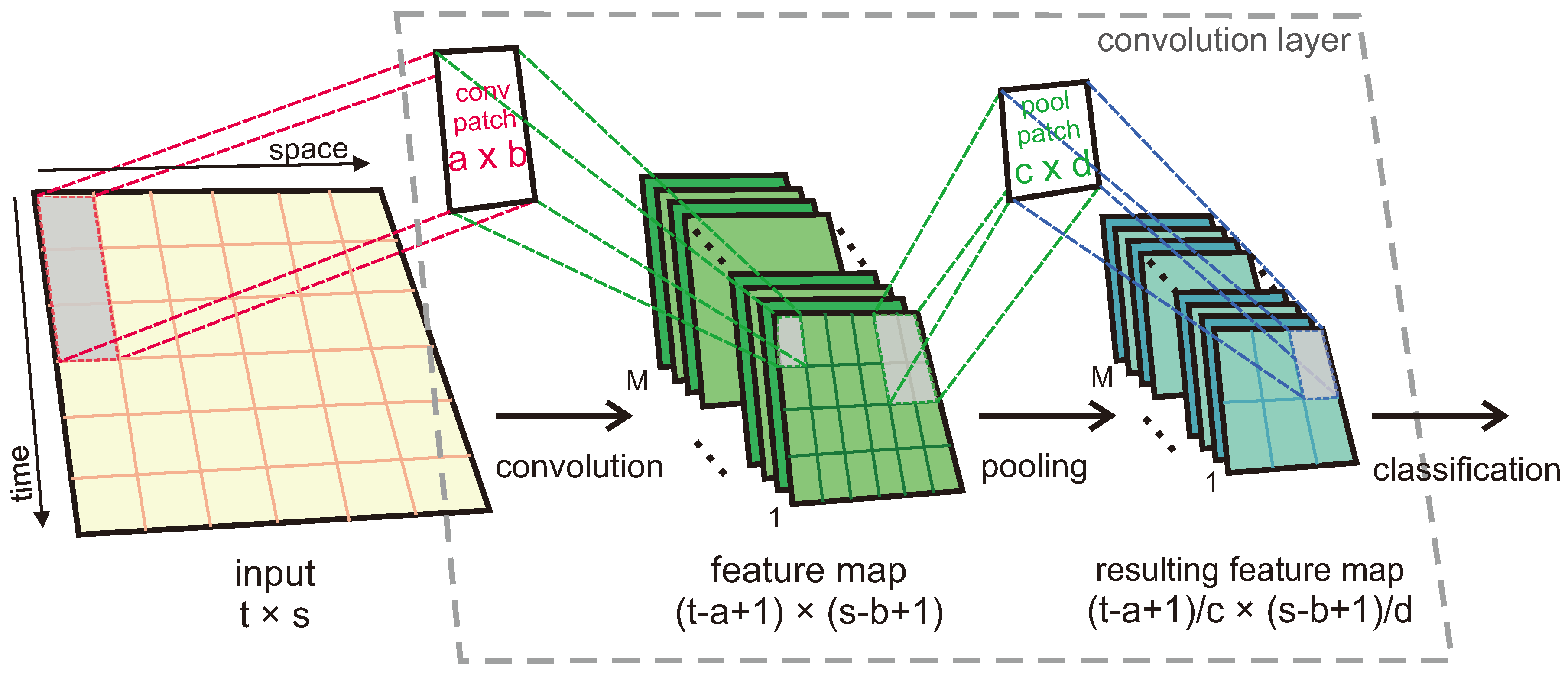
This particular neural network architecture is a type of multilayer perceptron with a feature-generation and a dimension-reduction -oriented layer, which, together, compose what is called a convolutional layer. Unlike other layer-based neural networks, the CNN can receive a multidimensional input in its original form, process it and successfully classify it without a previous feature extraction step. This is possible because the features are generated within the CNN layers, preventing possible information loss caused by user-created features or data rearrangement. Figure 2 shows the process an input experiences before classification by one of our proposed CNN models.
The convolution and pooling processes consist of applying patches (also known as kernels) to the input or the result from the previous patch application to extract features and reduce their sizes. For our study, a number of feature maps is produced as a result of the applications of such patches, each producing a feature map different from the other ones as the weights of the patches change. If an input, convolution patch and pool patch with sizes of , and , respectively, are considered, the convolution patch is first applied to the input to extract features of interest, which generates a feature map of size . Then, the pooling process takes place, which in our case is max pooling. By taking a single desired value out of an area (of the feature map) defined by the size of the pool patch, this process generates a resulting feature map of size for those cases in which the pooling process does not overlap. For our case , , change depending on the patches being used. The resulting feature maps are then connected to the output layer in which classification takes place. While in the convolution process, the applied patches overlap, that is not normally the case for the pooling process (see Section 3.1.3 for details). In this study, we test also CNN structures that cause the pool patches to overlap. The convolution and pooling processes occur as many times as there are convolution layers in the CNN.
3.1. Proposed Structures
As with other neural network structures, there are several CNN parameters to be defined by the user that will directly impact CNN performance. In this study, we considered as variables the number of convolutional layers and the shape of convolutional and pool patches. However, the learning rate, experiment stopping conditions, pool stride and optimization method are always the same regardless of the structure being tested. By proposing variations to the above-mentioned parameters, we were able to evaluate 18 different CNN structures in terms of classification rate. Figure 2 shows the general structure of the CNN used in this study.
3.1.1. Number of Convolution Layers
We propose structures with one and two convolution layers. This is the biggest structural difference the proposed models could exhibit as it heavily affects the size of the resulting feature maps. Structures with more than two convolution layers are not advised for applications such as ours, as early tests showed that the input was over simplified and the classification rate highly affected in a negative way.
3.1.2. Shape of Convolution and Pool Patches
Each of the EEG electrodes experiences the presence of the P300 wave in different magnitudes, and there are certain regions that are more likely to show it. This has been reported by different studies [14,25]. However, in most studies that attempt to classify EEG data, the two-dimensional position of the channels along the scalp of the user is mapped, generating a one-dimensional array that positions channels from different regions of the brain next to one another.
Given that applying either of the kernels in a squared-shaped fashion like that demonstrated in Figure 2 will result in feature maps that mix data from both the space and time domains, it is advised [14] that patches be constructed such that they only consider information of one dimension and one channel at a time. In this study, we considered three different convolution and pool patch sizes, including one pool patch that considers data from two adjacent channels simultaneously in the one-dimensional array. These patch sizes were chosen as a result of preliminary tests, in which a wide number of options was analyzed using data from one subject. The different CNN structures that were tested for this study consist of combinations of the selected number of layers and sizes of convolution and pool patches, which are summarized in Table 1. For a given number of convolution layers, the nine possible combinations of convolution and pool patches are considered. For the CNN with two layers, the same combination of convolution and pool patches is used in each layer. For the pooling operation, max pooling is applied.
For easier identification within the text, we will use brackets to refer to the patches listed above, e.g., pool patch []. The convolution layers will only be referred to as layers in the following sections. In this study, 64 feature maps of the same size are generated after the convolution.
3.1.3. Pool Stride
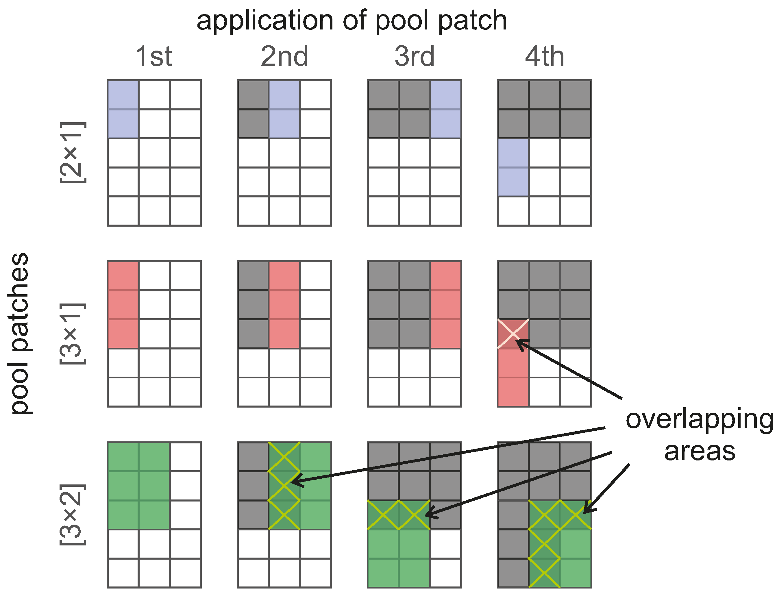
For this study, a fixed pool stride of size was considered for all 18 proposed CNN structures. Normally, the pool stride is the same size as the pool patch, which means that the pool process takes place in areas of the data that do not overlap. However, in early tests, that approach proved to be inadequate especially for the structures with two convolution layers. A fixed pool stride as the one proposed in this study implies that the area in which the pool kernels are applied overlap for the and the pool patches. The consequences of fixing the pool stride for the proposed pool patches can be seen in Figure 3, where the gray areas are those that the pool process has already considered, while the dark-colored ones correspond to those areas considered more than once (overlap) in the current application of the pool patches. Regardless of the pool patch size, their application occurs one space to the right of the previous one at a time and, when meeting the end of the structure, going back to the start, but spaced two spaces vertically. Although the consequences of the overlapping pooling process are still unknown in the application of CNN in BCI, this approach has successfully been used for image recognition [23]. With the selected size of the fixed pool stride and the proposed pool patches, we can account for CNN that do not experience overlapping in the case of pool patch , other ones that do experience overlap for the patch and, finally, models that experience overlapping and also consider data from two channels simultaneously, which corresponds to the pool patch . Depending on the pool strategy used, the size of the resulting feature map varies slightly.
3.1.4. Learning Rate
The discussion towards learning rate usually goes in two directions: whether it is chosen based on how fast it is desired for the training to be finished or depending on the size of each example in the dataset. The learning rate used for this study is 0.008. Several other learning rate values ranging from 0.1 to 0.000001 were tested in preliminary tests with noticeable negative repercussions for CNN performance, either with respect to the time required to train or the overall classification rate. The value was chosen as it allows one to see gradual and meaningful changes in the accuracy rate evolution during both training and test phases.
3.1.5. Optimization Method
We used stochastic gradient descent (SGD) to minimize the error present during training. The work of [27] has demonstrated that this method is useful for training neural networks on large datasets. For this case, the error function is given as a sum of terms for a set of independent observations , one for each example or batch of examples in the dataset being used in the form:
Thus, making the weight updates based on one example or batch of examples at a time, such that:
where w is the weight and bias of the network grouped together (weight vector), is the number of iterations of the learning process in the neural network, is the learning rate and n ranges from one to Q, which is the maximum number of examples or possible batches in the provided set depending on whether the batch approach is used or not. For this study, batches of 100 examples were used when training any of the proposed CNN structures.
3.1.6. Output Classification
We used a softmax function to evaluate the probability of the input x belonging to each of the possible classes. This is done by:
where is the current class being considered, and , where L represents the maximum number of classes. After the probability is computed for each class, the highest value is forced to one and the rest to zero, forming a vector of the same size as the provided teaching vector (labels). The vectors are then compared to see if the suggested class is the same as the one given as the teaching vector.
3.1.7. Accuracy Rate
As the data-sets used for training and testing the different CNN contained examples for two classes of stimuli (target and non-target) in different amounts, the accuracy rate is defined by the expression:
which heavily penalizes poor individual classification performance in binary classification tasks. TP stands for true positives and is the number of correctly classified target examples, and TN, which stands for true negatives, is the number of correctly classified non-target examples. P and N represent the total number of examples of the target and non-target classes, respectively, for this case.
All the CNN structures were implemented using a GeForce GTX TITAN X GPU by NVIDIA in Python 2.7 using the work developed by [28].
4. Results for P300 Identification
In this section, we compare the obtained results from the 72 CNN models (18 for each of the four trial intervals) and group them in two different ways in order to facilitate the appreciation of patterns of interest. First, the obtained accuracy rates with fixed convolution patches as seen in Table 2 are discussed. Then, we describe the results of models with fixed pool patches, as shown in Table 3. These two ways of presenting the same results allows one to recognize some performance patterns linked to the convolution or pool patches used for each model. The results show the mean accuracy of each model for the nine subjects that took part in the experiment. At the same time, the results are the mean value obtained from a two-fold cross-validation, where the accuracy for each fold was calculated using Equation (4).
The highest accuracy rate obtained among all the tested models was 0.927 for trials 500 ms long in the model with one layer, convolution patch [] and pool patch []. The lowest accuracy rate was 0.783 for trials 200 ms long in the model with two layers, convolution patch [] and pool patch [].
4.1. Fixed Convolution Patches
Producing good results by mixing information from two adjacent channels in a mapped channel vector was considered with skepticism. However, if a direct comparison between the structures with different pool patches is considered (see Table 2), in all cases but one for the one-layered structures and considering all trial lengths, the best results were obtained by those models using the pool patch [], which considers both spatial and temporal information. This behavior is not seen for models that use two layers. Additionally, regardless of the number of layers, 58.3% (42 models) of the time, the best results were from structures that used pool patch [], 25% (18 models) of the time for when pool patch [] was applied and 16.6% (12 models) of the time for structures that used pool patch [].
With respect to the convolution patch [] for trials 200 ms long, the lowest accuracy corresponded to the structure with one layer and pool patch []. In this condition, an accuracy rate of 0.915 was also achieved by another structure (one layer and pool patch []), thus representing the biggest accuracy rate gap (around 13%) among results produced for a trial of the same length and convolution patch.
4.2. Fixed Pool Patches
In Table 3, the results are now accommodated by fixing the pool patches. Comparing results between different convolution patches on the structures with one and two layers separately reveals a tendency for the convolution patch [] to offer the best accuracy rates for 70.8% of the cases (51 models). As for the convolution patches [] and [], for 16.6% (12 models) and 12.5% (9 models) of the time, they produce the best results, respectively. If only the two-layer models are considered, the convolution patch [] offers the best results for all cases except one (the model with and ), similar to the pattern for the one-layer models in Table 2 discussed before.
4.3. Mean Accuracy Rate for Fixed Patches
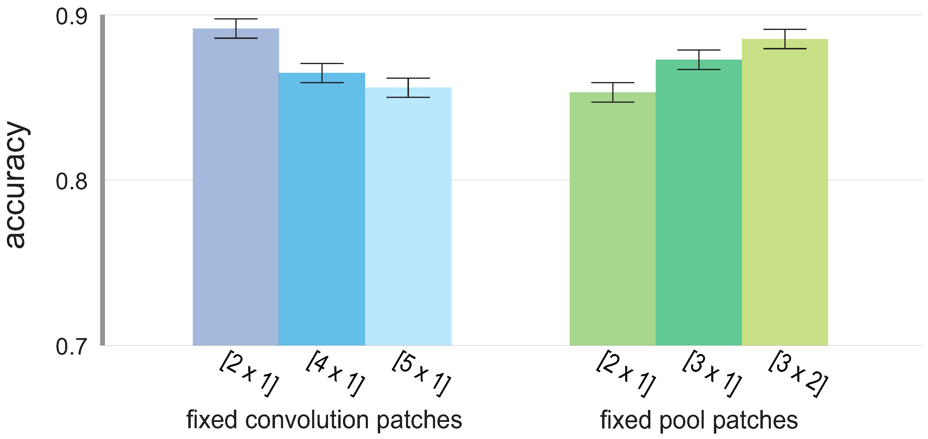
Given the fixed convolution or pool patches presented in Table 2 and Table 3, the mean accuracy for all possible CNN models is presented in Figure 4 to show the differences in patch performance.
For the convolution patches, achieved the overall highest accuracy (presented with the standard deviation), i.e., with , followed by and , in that order, with and , respectively. As for the pool patches, the approach in which the pool patch is the same size as the pool stride, i.e., no overlapping occurs, yielded the lowest overall accuracy at , followed by , the patch representing the overlapping pool process, with , and finally, by the pool patch that not only causes overlap, but also considers data from two adjacent channels in the mapped version of the channels, , with .
5. Discussion
In this study, we proposed and tested the efficacy of 18 different CNN for classifying the presence or absence of the P300 wave from the EEG readings of nine subjects in an auditory BCI with virtual direction sources. We approached the classification task by testing three pooling strategies and considering four different trial lengths for the presentation of the auditory stimuli. The implementation of the mentioned strategies is possible due to the fixed pooling stride explained in Section 3.1.3 and present in all of the CNN models. The fixed pooling stride also prevents the resulting feature maps from being oversimplified, as having a stride that matches the size of the pooling kernel might not be possible in all cases due to the down-sampling of the data.
5.1. Pooling Strategies and Other Studies
The first pooling strategy, represented by pool patch , is the most common approach used in CNN and consists of a pooling process in which the pool patch and stride are of the same size. In this study, this approach led to the lowest general accuracy rates.
The goal of the second strategy, represented by , is to cause overlapping of the pool patches. This strategy has been tested in previous work, although with data of a very different nature. While [24] reported no differences between performance for approaches with or without overlapping for speech tasks, we have found that, as in the work of [27], better CNN model performance can be achieved using an overlapping pool strategy.
The third strategy, represented by pool patch , showed that the performance of the overlapping strategy can be further enhanced by also considering data from two different adjacent channels simultaneously. This consideration is not applied to the original input, but rather to feature maps generated after the convolution patch is applied.
Past studies involving the classification of single-trial P300 includes the work of [14], in which results are reported for P300 identification using raw data from Dataset II from the third BCI competition [17]. Rather than changing the parameters of a CNN model, they presented the results of changing the way the input is constructed. In the best scenario, they achieve accuracy rates of 0.7038 and 0.7819 for each of two subjects, with a mean accuracy of 0.7428. In the work of [29], three experiments were conducted, which compared different classifiers for classification of single-trial ERPs for rapid serial visual presentation (RSVP) tasks. They found that the best performance is achieved by a CNN, with a mean accuracy and standard deviation of . Another RSVP task is presented in [21] where CNNs are also used for classification. By applying the CNN classifier, they found that they could improve the results obtained in previous studies. These studies are well known, but were not focused on single-trial P300 classification; however, they present approaches that inspired this work and provide a reference to what has normally been achieved in this context.
In [25], single trial P300 classification is reported as part of their results. By using support vector machines (SVM), they achieve a mean accuracy rate of approximately 0.70 for seven subjects when considering a reduced number of EEG channels. Another case of a single-trial identification attempt comes from [30], where Fisher’s discriminant analysis (FDA) regularized parameters are searched for using particle swarm optimization, achieving an accuracy of 0.745 for single trials and no channel selection. These results can be fairly compared to ours (see Section 5.4), as the goal of these studies, their experimental setup and BCI approach are the same as the ones we present.
In this study, the highest mean accuracy rate for nine subjects was 0.927, and the lowest was 0.783. The mean accuracy rates for all the models for fixed trial intervals were , , and for the 200-, 300-, 400- and 500-ms trial interval, respectively.
5.2. Convolution Patches and Number of Layers
Although we approached this study expecting the pooling strategies to play the most relevant role performance-wise, we also observed patterns of improvement depending on the selected convolution patch (as presented in Figure 4) and the number of layers. Considering less information in the time domain for the convolution process leads to better mean accuracy rates. We found the difference between the highest and lowest mean accuracy rate in the convolution patch to be 0.036, which is slightly bigger than the difference between the lowest and highest mean accuracy rates between the tested pool strategies (0.032).
On a related matter, the models with only one layer outperformed those with two layers in 21 (58.3%) of the 36 cases. As each time the pool patch is applied, the size of the input is reduced significantly, a large number of layers might produce an oversimplification of the input. In our preliminary research, models with three and four layers were tested for different tasks using the datasets described in this work; however, they performed poorly in comparison to models with only one or two layers. This situation might be different if the input we used did not consist of down-sampled data, therefore not falling into the oversimplification problem with the proposed CNN models.
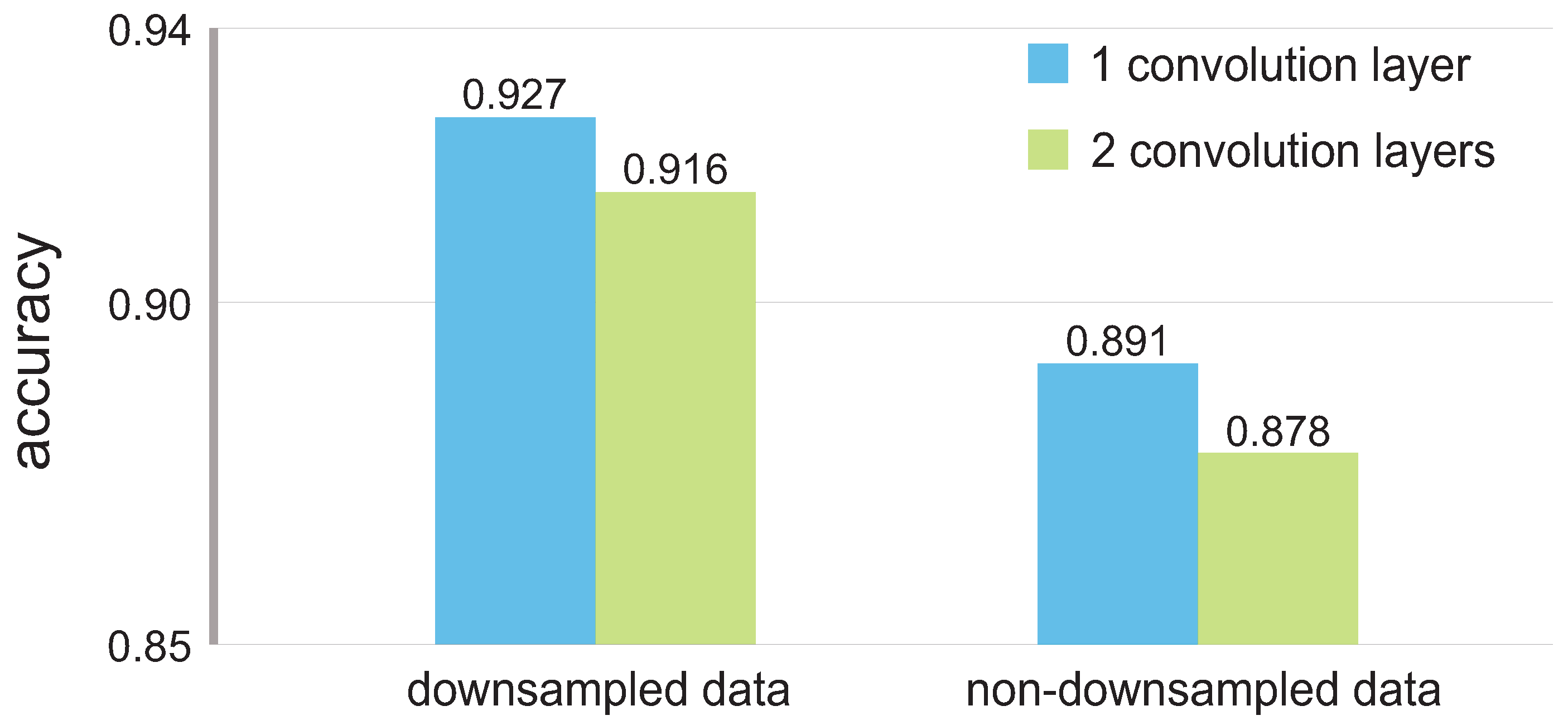
To analyze whether the down-sampling negatively affects the performance of the CNN, we used non-down-sampled data to test the model that achieved the highest accuracy as reported in Section 4. The results, which favor the down-sampled data, can be seen in Figure 5.
By using down-sampled data, we could not only boost the accuracy with respect to the non-down-sampled data, but also shorten the training/testing times inherent in the size of the input.
5.3. Alternative Training Approach
For the results presented in Section 4, we used the training approach ‘single subject approach’ described in Section 5.3.1 trying to achieve the best possible performance. However, the ‘combined subjects approach’ described in Section 5.3.2 is also a viable way to address CNN training. Next, we will discuss the differences between both approaches and offer results that support our decision to implement the former.
5.3.1. Single-Subject Approach
This approach consists of training one CNN using the data of a single subject at a time for each trial length. As the ability to correctly recognize irregular auditory cues varies from one subject to another, this approach allows some of the trained CNN models to perform particularly well if the data come from a subject that excelled in the recognition task. The drawback of using this approach is the large amount of time needed to obtain the mean accuracy of a single CNN model as each of the proposed structures is trained individually for each subject. Therefore, considering a single trial length, CNN were trained. The mean accuracy rate obtained for all subjects is presented as the result for a single CNN model. The average time spent on training was about 20 min for the structures with one convolution layer and approximately 27 min for those with two layers.
5.3.2. Combined Subjects Approach
This approach consists of training only one CNN with examples from all of the subjects for each different trial length and then testing each subject individually on the trained CNN. This approach allows one to decrease the number of CNN to train in order to obtain the average accuracy rate for a single CNN model and therefore the time needed to analyze the results. Using this approach also means that the number of examples for training and testing will increase by the number of subjects. A major drawback of this approach is that subjects who fail to recognize the irregular auditory cues will produce examples that do not contain the P300 even if they are labeled otherwise, negatively affecting the CNN performance. For a single CNN model considering data from all subjects, the average time spent on training was about 32 min for the structures with one convolution layer and approximately 39 for those with two layers.
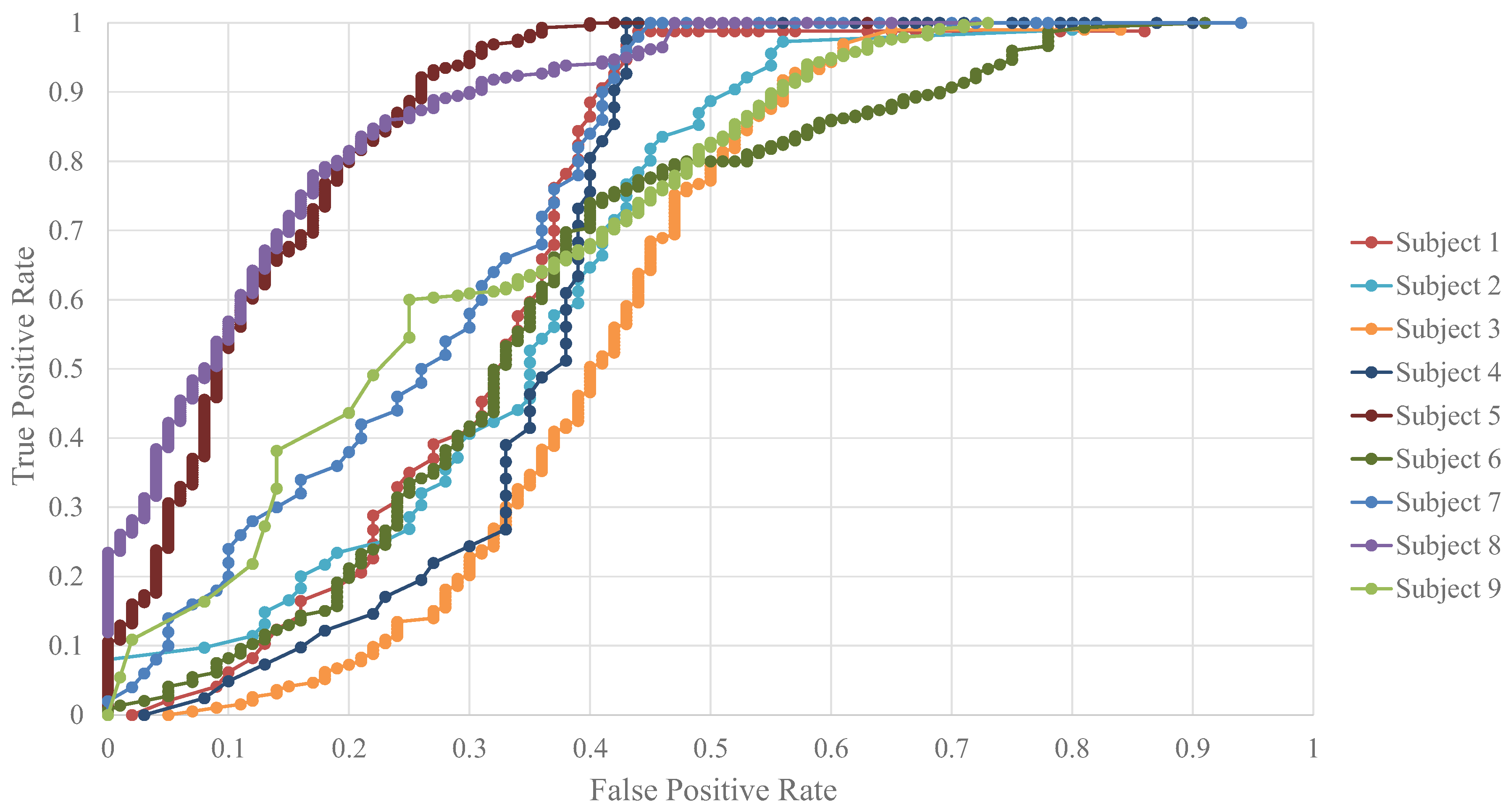
The model that exhibited the best performance in Section 4 was chosen to be tested using also the previously explained combined subjects approach to determine if it offered better performance than that of the currently used approach. Table 4 shows the comparison between the results for the single subject and combined subjects approaches for each subject considering the CNN structure with the overall highest accuracy rate (one layer, convolution patch , pool patch ). The difference in the mean accuracy rate is about 6%, in favor of the single-subject approach. If subjects are compared in terms of the two approaches, the combined subjects approach is better only in one out of the nine cases. Subject 9, which produced the lowest accuracy in the single-subject approach, benefited slightly from the combined subjects approach. In the eight cases in which the single-subject approach obtains better results, the accuracy rates between both approaches varies between 0% and 11%, depending on the subject. Figure 6 shows the receiver operating characteristic (ROC) curves for each of the nine subjects for the CNN model with the highest accuracy under the single-subject approach. These curves can serve to better understand the results presented in Table 4 for such an approach.
Although there is a substantial difference between both approaches of about five times in terms of the amount of time each one required to produce the mean accuracy, the single-subject approach offered better results.
5.4. CNN and Other Classifiers
As presented in Section 5.1, there are many studies related somehow to the one we present now. We considered it appropriate to compare some of the classifiers those works present that are not CNN. To compare the obtained results from the CNN with other classifiers, we used support vector machines (SVM) and Fisher’s discriminant analysis (FDA) for all of the available trial lengths. Details for how we implemented these two classifiers can be found in the Appendix. Table 5 shows the comparison between the accuracy, precision and recall results obtained from the SVM, FDA and the CNN model that achieved the highest accuracy rate in four different trial intervals: 200, 300, 400 and 500 ms.
The results from CNN with the highest accuracy compared to those of the SVM or the FDA are clearly higher, and this difference decreases if we take into consideration the lowest accuracy obtained by one of our CNN models, which is 0.783, with a precision of 1.0 and a recall of 0.618 for the 200-ms trial interval.
5.5. Future Work
Like many previous studies, we used a mapped version of the EEG channels to create a two-dimensional input for CNN. However, EEG data, especially those recorded during experiments conducted using the oddball paradigm, exhibit areas where irregular events have more visible repercussions. For this reason, it is of interest in the future for EEG analysis that the input of the CNN is a three-dimensional structure. Images have this kind of topology, in which two dimensions are used for the position of pixels and three channels define the color of a given pixel. Thus, instead of analyzing one channel at a time to avoid mixing spatial and temporal information, larger two-dimensional patches could be used in both the convolution and pooling process to address a specific moment in the EEG readings. The result would be a map showing the complete brain activity in that particular point.
Embracing different training schemes to reduce the computation time needed for the results to be obtained should be considered. The presented accuracy rates were obtained by training and testing a CNN for each subject on each of the proposed structures and repeating that for the different trial lengths, resulting in long training sessions to obtain the mean accuracy rate of a single structure.
6. Conclusions
By proposing and testing CNN models to classify single-trial P300 waves, we obtained state of the art performances for CNN models using different pooling strategies in the form of mean accuracy rates for nine subjects. We proved that, in off-line classification, single-trial P300 examples could be correctly classified in the auditory BCI we proposed, which uses headphones to produce sound from six virtual directions, thus reducing the amount of hardware needed to implement the BCI in real life. While similar previous studies obtained accuracy rates varying from approximately 0.70 to 0.745, we found mean accuracy rates ranging from 0.855 to 0.888 depending on the trial interval and from 0.783 to 0.927 if individual models are considered. We achieved this by applying different pooling strategies that affect the performance of CNN models dealing with EEG data for classification purposes, as well as using a different number of convolution layers. We found that either of the approaches that overlap in the pooling process or also consider data from two adjacent channels performed better than the most common approach, which uses a pooling stride that is the same size as the pool patch and only considers data from one channel at a time. In most cases, models with simple structures (only one layer) perform better for this type of case and also offer faster training times. Other improvement patterns were also observed for the different convolution patches, as well as for how to approach the training and testing of CNN models.
Acknowledgments
This work was supported in part by Nagaoka University of Technology Presidential Grant and JSPS Kakenhi, Grants 24300051, 24650104 and 16K00182.
Author Contributions
Wada Yasuhiro, Isao Nambu and Miho Sugi conceived of and designed the experiments. Miho Sugi performed the experiments. Eduardo Carabez analyzed the data. Wada Yasuhiro, Isao Nambu and Eduardo Carabez wrote the paper.
Conflicts of Interest
The authors declare no conflict of interest.
Appendix A
SVM
Analysis was performed using LIBSVM software [31] and implemented in MATLAB (MathWorks, Natick, MA, USA). We used a weighted linear SVM [32] to compensate for imbalance in the target and non-target examples. Thus, we used a penalty parameter of C+ for the target and C-for the non-target examples. The penalty parameter for each class was searched in the range of to ( ≤ 10 ≤ ; m: −6:0.5:−1) within the training. We determined the best parameters as those that obtained the highest accuracy using 10-fold cross-validation for the training. Using the best penalty parameters, we constructed the SVM classifier using all training data and applied it to the test data.
FDA
We used a variant of the regularized Fisher discriminant analysis (FDA) as the classification algorithm [30]. In this algorithm, a regularized parameter for FDA is searched for by particle swarm optimization (for details, see [30]) within the training. In this study, we used all EEG channels without selection.
References
- He, B.; Gao, S.; Yuan, H.; Wolpaw, J.R. Brain-computer interfaces. In Neural Engineering; Springer: Berlin/Heidelberg, Germany, 2013; pp. 87–151. [Google Scholar]
- Nijboer, F.; Furdea, A.; Gunst, I.; Mellinger, J.; McFarland, D.J.; Birbaumer, N.; Kübler, A. An auditory brain-computer interface BCI. J. Neurosci. Methods 2008, 167, 43–50. [Google Scholar] [CrossRef] [PubMed]
- Vos, M.D.; Gandras, K.; Debener, S. Towards a truly mobile auditory brain-computer interface: Exploring the P300 to take away. Int. J. Psychophysiol. 2014, 91, 46–53. [Google Scholar] [CrossRef] [PubMed]
- Allison, B.Z.; McFarland, D.J.; Schalk, G.; Zheng, S.D.; Jackson, M.M.; Wolpaw, J.R. Towards an independent brain-computer interface using steady state visual evoked potentials. Clin. Neurophysiol. 2008, 119, 399–408. [Google Scholar] [CrossRef] [PubMed]
- Käthner, I.; Ruf, C.A.; Pasqualotto, E.; Braun, C.; Birbaumer, N.; Halder, S. A portable auditory P300 brain-computer interface with directional cues. Clin. Neurophysiol. 2013, 124, 327–338. [Google Scholar] [CrossRef] [PubMed]
- Citi, L.; Poli, R.; Cinel, C.; Sepulveda, F. L300-Based BCI Mouse With Genetically-Optimized Analogue Control. IEEE Trans. Neural Syst. Rehabil. Eng. 2008, 16, 51–61. [Google Scholar] [CrossRef] [PubMed] [Green Version]
- Rebsamen, B.; Burdet, E.; Guan, C.; Zhang, H.; Teo, C.L.; Zeng, Q.; Laugier, C.; Ang, M.H., Jr. Controlling a Wheelchair Indoors Using Thought. IEEE Intell. Syst. 2007, 22, 18–24. [Google Scholar] [CrossRef]
- Nijboer, F.; Birbaumer, N.; Kübler, A. The Influence of Psychological State and Motivation on Brain-Computer Interface Performance in Patients with Amyotrophic Lateral Sclerosis—A Longitudinal Study. Front. Neurosci. 2010, 4. [Google Scholar] [CrossRef] [PubMed]
- Baykara, E.; Ruf, C.A.; Fioravanti, C.; Käthner, I.; Simon, N.; Kleih, S.C.; Kübler, A.; Halder, S. Effects of training and motivation on auditory P300 brain-computer interface performance. Clin. Neurophysiol. 2016, 127, 379–387. [Google Scholar] [CrossRef] [PubMed]
- Sellers, E.W.; Donchin, E. A P300-based brain-computer interface: Initial tests by ALS patients. Clin. Neurophysiol. 2006, 117, 538–548. [Google Scholar] [CrossRef] [PubMed]
- Chang, M.; Nishikawa, N.; Struzik, Z.R.; Mori, K.; Makino, S.; Mandic, D.; Rutkowski, T.M. Comparison of P300 Responses in Auditory, Visual and Audiovisual Spatial Speller BCI Paradigms. arXiv, 2013; arXiv:q-bio.NC/1301.6360. [Google Scholar]
- Hoffmann, U.; Vesin, J.M.; Ebrahimi, T.; Diserens, K. An efficient P300-based brain-computer interface for disabled subjects. J. Neurosci. Methods 2008, 167, 115–125. [Google Scholar] [CrossRef] [PubMed]
- Nijboer, F.; Sellers, E.W.; Mellinger, J.; Jordan, M.A.; Matuz, T.; Furdea, A.; Halder, S.; Mochty, U.; Krusienski, D.J.; Vaughan, T.M.; et al. A P300-based brain-computer interface for people with amyotrophic lateral sclerosis. Clin. Neurophysiol. 2008, 119, 1909–1916. [Google Scholar] [CrossRef] [PubMed]
- Cecotti, H.; Gräser, A. Convolutional Neural Networks for P300 Detection with Application to Brain-Computer Interfaces. IEEE Trans. Pattern Anal. Mach. Intell. 2011, 33, 433–445. [Google Scholar] [CrossRef] [PubMed]
- Cecotti, H.; Gräser, A. Time Delay Neural Network with Fourier transform for multiple channel detection of Steady-State Visual Evoked Potentials for Brain-Computer Interfaces. In Proceedings of the 2008 16th European Signal Processing Conference, Lausanne, Switzerland, 25–29 August 2008; pp. 1–5. [Google Scholar]
- Guler, I.; Ubeyli, E.D. Multiclass Support Vector Machines for EEG-Signals Classification. IEEE Trans. Inf. Technol. Biomed. 2007, 11, 117–126. [Google Scholar] [CrossRef] [PubMed]
- Kaper, M.; Meinicke, P.; Grossekathoefer, U.; Lingner, T.; Ritter, H. BCI competition 2003-data set IIb: Support vector machines for the P300 speller paradigm. IEEE Trans. Biomed. Eng. 2004, 51, 1073–1076. [Google Scholar] [CrossRef] [PubMed]
- Naseer, N.; Qureshi, N.K.; Noori, F.M.; Hong, K.S. Analysis of different classification techniques for two-class functional near-infrared spectroscopy-based brain-computer interface. Comput. Intell. Neurosci. 2016, 2016. [Google Scholar] [CrossRef] [PubMed]
- Abdel-Hamid, O.; Deng, L.; Yu, D. Exploring convolutional neural network structures and optimization techniques for speech recognition. In Proceedings of the 14th Annual Conference of the International Speech Communication Association, Lyon, France, 25–29 August 2013; pp. 3366–3370. [Google Scholar]
- Simonyan, K.; Zisserman, A. Very Deep Convolutional Networks for Large-Scale Image Recognition. arXiv, 2014; arXiv:1409.1556. [Google Scholar]
- Manor, R.; Geva, A.B. Convolutional Neural Network for Multi-Category Rapid Serial Visual Presentation BCI. Front. Comput. Neurosci. 2015, 9. [Google Scholar] [CrossRef] [PubMed]
- Bevilacqua, V.; Tattoli, G.; Buongiorno, D.; Loconsole, C.; Leonardis, D.; Barsotti, M.; Frisoli, A.; Bergamasco, M. A novel BCI-SSVEP based approach for control of walking in Virtual Environment using a Convolutional Neural Network. In Proceedings of the 2014 International Joint Conference on Neural Networks (IJCNN), Beijing, China, 6–11 July 2014; pp. 4121–4128. [Google Scholar]
- Krizhevsky, A.; Sutskever, I.; Hinton, G.E. ImageNet Classification with Deep Convolutional Neural Networks. In Advances in Neural Information Processing Systems 25; Pereira, F., Burges, C.J.C., Bottou, L., Weinberger, K.Q., Eds.; Curran Associates, Inc.: Red Hook, NY, USA, 2012; pp. 1097–1105. [Google Scholar]
- Sainath, T.N.; Kingsbury, B.; Saon, G.; Soltau, H.; Mohamed, A.; Dahl, G.; Ramabhadran, B. Deep Convolutional Neural Networks for Large-scale Speech Tasks. Neural Netw. 2015, 64, 39–48. [Google Scholar] [CrossRef] [PubMed]
- Nambu, I.; Ebisawa, M.; Kogure, M.; Yano, S.; Hokari, H.; Wada, Y. Estimating the Intended Sound Direction of the User: Toward an Auditory Brain-Computer Interface Using Out-of-Head Sound Localization. PLoS ONE 2013, 8, 1–14. [Google Scholar] [CrossRef] [PubMed]
- Yano, S.; Hokari, H.; Shimada, S. A study on personal difference in the transfer functions of sound localization using stereo earphones. IEICE Trans. Fundam. Electron. Commun. Comput. Sci. 2000, 83, 877–887. [Google Scholar]
- LeCun, Y.; Boser, B.; Denker, J.S.; Henderson, D.; Howard, R.E.; Hubbard, W.; Jackel, L.D. Backpropagation applied to handwritten zip code recognition. Neural Comput. 1989, 1, 541–551. [Google Scholar] [CrossRef]
- Goodfellow, I.J.; Warde-Farley, D.; Lamblin, P.; Dumoulin, V.; Mirza, M.; Pascanu, R.; Bergstra, J.; Bastien, F.; Bengio, Y. Pylearn2: A machine learning research library. arXiv, 2013; arXiv:stat.ML/1308.4214. [Google Scholar]
- Cecotti, H.; Eckstein, M.P.; Giesbrecht, B. Single-Trial Classification of Event-Related Potentials in Rapid Serial Visual Presentation Tasks Using Supervised Spatial Filtering. IEEE Trans. Neural Netw. Learn. Syst. 2014, 25, 2030–2042. [Google Scholar] [CrossRef] [PubMed]
- Gonzalez, A.; Nambu, I.; Hokari, H.; Wada, Y. EEG channel selection using particle swarm optimization for the classification of auditory event-related potentials. Sci. World J. 2014, 2014. [Google Scholar] [CrossRef] [PubMed]
- Chang, C.; Lin, C. LIBSVM: A library for support vector machines. ACM Trans. Intell. Syst. Technol. (TIST) 2011, 2. [Google Scholar] [CrossRef]
- Osuna, E.; Freund, R.; Girosi, F. An improved training algorithm for support vector machines. In Proceedings of the 1997 IEEE Signal Processing Society Workshop on Neural Networks for Signal Processing VII, Amelia Island, FL, USA, 24–26 September 1997; pp. 276–285. [Google Scholar]
Figure 1.
(a) 64 electroencephalogram (EEG) channel layout used in the experiments. Reference electrodes attached to the ears; (b) Virtual disposition of the six sound directions with respect to the user. A stimulus is being produced from Direction 3; (c) Task constitution.
Figure 1.
(a) 64 electroencephalogram (EEG) channel layout used in the experiments. Reference electrodes attached to the ears; (b) Virtual disposition of the six sound directions with respect to the user. A stimulus is being produced from Direction 3; (c) Task constitution.
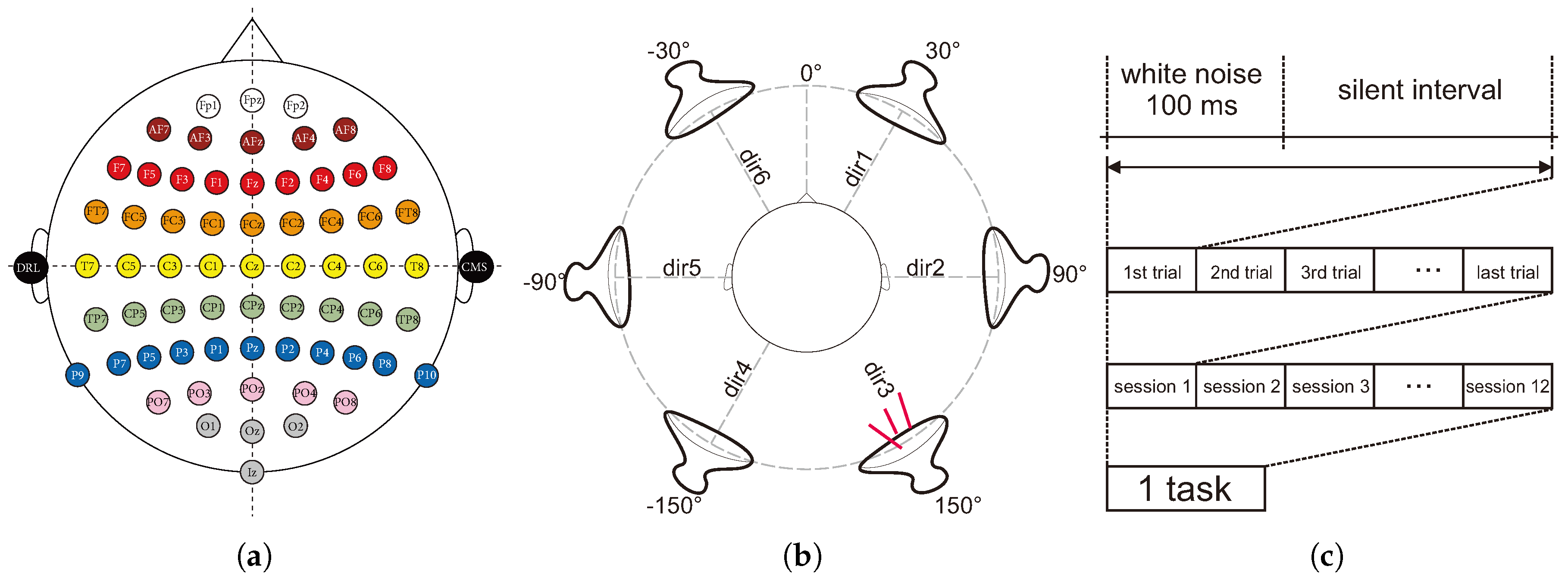
Figure 2.
Structure of a convolutional neural network (CNN) depicting the results of applying the convolution and pooling processes in the convolution layer for the input. Default pooling (non-overlapping) is shown in this figure.
Figure 2.
Structure of a convolutional neural network (CNN) depicting the results of applying the convolution and pooling processes in the convolution layer for the input. Default pooling (non-overlapping) is shown in this figure.

Figure 3.
Proposed pooling patches applied on a structure to show overlapping caused by the fixed pooling stride. Gray areas represent those in which the patch has been applied, and dark-colored areas are those in which the patch overlaps with previous iterations.
Figure 3.
Proposed pooling patches applied on a structure to show overlapping caused by the fixed pooling stride. Gray areas represent those in which the patch has been applied, and dark-colored areas are those in which the patch overlaps with previous iterations.

Figure 4.
Mean accuracy, along with the accuracy’s standard deviation, for all models with fixed convolution patches (left) and pool patches (right).
Figure 4.
Mean accuracy, along with the accuracy’s standard deviation, for all models with fixed convolution patches (left) and pool patches (right).

Figure 5.
Difference in mean accuracy for the model with the highest performance using down-sampled and non-down-sampled data.
Figure 5.
Difference in mean accuracy for the model with the highest performance using down-sampled and non-down-sampled data.

Figure 6.
Receiver operating characteristic (ROC) curves of each subject for the CNN model with one layer, convolution patch [] and pool patch [] using the single-subject approach.
Figure 6.
Receiver operating characteristic (ROC) curves of each subject for the CNN model with one layer, convolution patch [] and pool patch [] using the single-subject approach.

Table 1.
Proposed and tested number of convolution layers, size of convolution patches and size of pool patches.
Table 1.
Proposed and tested number of convolution layers, size of convolution patches and size of pool patches.
| Convolution Layers | 1 | 2 | |
|---|---|---|---|
| Size of convolution patch | |||
| Size of pool patch | |||
Table 2.
Summarized results for the 18 convolutional neural networks (CNN) structures for all considered trial lengths with fixed convolution patches. PP = pool patch, CP = convolution patch, CL = convolution layers.
Table 2.
Summarized results for the 18 convolutional neural networks (CNN) structures for all considered trial lengths with fixed convolution patches. PP = pool patch, CP = convolution patch, CL = convolution layers.
| 500 ms | 400 ms | 300 ms | 200 ms | ||||||
|---|---|---|---|---|---|---|---|---|---|
| CP | PP | CL 1 | CL 2 | CL 1 | CL 2 | CL 1 | CL 2 | CL 1 | CL 2 |
| 0.882 | 0.915 | 0.860 | 0.914 | 0.850 | 0.903 | 0.842 | 0.880 | ||
| 0.920 | 0.910 | 0.899 | 0.906 | 0.865 | 0.883 | 0.880 | 0.891 | ||
| 0.907 | 0.910 | 0.919 | 0.906 | 0.881 | 0.884 | 0.897 | 0.887 | ||
| 0.855 | 0.869 | 0.867 | 0.880 | 0.796 | 0.809 | 0.837 | 0.814 | ||
| 0.880 | 0.884 | 0.901 | 0.864 | 0.858 | 0.855 | 0.838 | 0.832 | ||
| 0.927 | 0.916 | 0.912 | 0.868 | 0.872 | 0.836 | 0.911 | 0.848 | ||
| 0.869 | 0.840 | 0.855 | 0.867 | 0.805 | 0.827 | 0.841 | 0.783 | ||
| 0.896 | 0.847 | 0.880 | 0.868 | 0.874 | 0.839 | 0.841 | 0.826 | ||
| 0.897 | 0.857 | 0.895 | 0.859 | 0.890 | 0.824 | 0.915 | 0.820 | ||
Table 3.
Summarized results for the 18 CNN structures for all considered trial lengths with fixed pool patches. PP = pool patch, CP = convolution patch, CL = convolution layers.
Table 3.
Summarized results for the 18 CNN structures for all considered trial lengths with fixed pool patches. PP = pool patch, CP = convolution patch, CL = convolution layers.
| 500 ms | 400 ms | 300 ms | 200 ms | ||||||
|---|---|---|---|---|---|---|---|---|---|
| PP | CP | CL 1 | CL 2 | CL 1 | CL 2 | CL 1 | CL 2 | CL 1 | CL 2 |
| 0.882 | 0.915 | 0.860 | 0.914 | 0.850 | 0.903 | 0.842 | 0.880 | ||
| 0.855 | 0.869 | 0.867 | 0.880 | 0.796 | 0.809 | 0.837 | 0.814 | ||
| 0.869 | 0.840 | 0.855 | 0.867 | 0.805 | 0.827 | 0.841 | 0.783 | ||
| 0.920 | 0.910 | 0.899 | 0.906 | 0.865 | 0.883 | 0.880 | 0.891 | ||
| 0.880 | 0.884 | 0.901 | 0.864 | 0.858 | 0.855 | 0.838 | 0.832 | ||
| 0.896 | 0.847 | 0.880 | 0.868 | 0.874 | 0.839 | 0.841 | 0.826 | ||
| 0.907 | 0.910 | 0.919 | 0.906 | 0.881 | 0.884 | 0.897 | 0.887 | ||
| 0.927 | 0.916 | 0.912 | 0.868 | 0.872 | 0.836 | 0.911 | 0.848 | ||
| 0.897 | 0.857 | 0.895 | 0.859 | 0.890 | 0.824 | 0.915 | 0.820 | ||
Table 4.
Comparison between the accuracy rates obtained for the single-subject (SS) and combined subject (CS) approaches for the CNN model with 1 layer, convolution patch [] and pool patch [].
Table 4.
Comparison between the accuracy rates obtained for the single-subject (SS) and combined subject (CS) approaches for the CNN model with 1 layer, convolution patch [] and pool patch [].
| 500 ms | ||
|---|---|---|
| Subject | SS | CS |
| 1 | 0.926 | 0.858 |
| 2 | 0.893 | 0.817 |
| 3 | 0.914 | 0.912 |
| 4 | 0.948 | 0.877 |
| 5 | 0.969 | 0.851 |
| 6 | 0.953 | 0.854 |
| 7 | 0.969 | 0.915 |
| 8 | 0.916 | 0.836 |
| 9 | 0.854 | 0.865 |
| Average accuracy | 0.927 | 0.865 |
Table 5.
Comparison between the overall accuracy rates, precision and recall obtained for the CNN model with the highest accuracy rate, support vector machines (SVM) and Fisher’s discriminant analysis (FDA).
Table 5.
Comparison between the overall accuracy rates, precision and recall obtained for the CNN model with the highest accuracy rate, support vector machines (SVM) and Fisher’s discriminant analysis (FDA).
| Accuracy | Precision | Recall | |||||||
|---|---|---|---|---|---|---|---|---|---|
| CNN | SVM | FDA | CNN | SVM | FDA | CNN | SVM | FDA | |
| 500 ms | 0.927 | 0.709 | 0.745 | 0.994 | 0.37 | 0.43 | 0.826 | 0.70 | 0.71 |
| 400 ms | 0.912 | 0.711 | 0.731 | 0.987 | 0.37 | 0.41 | 0.836 | 0.70 | 0.68 |
| 300 ms | 0.872 | 0.691 | 0.707 | 0.992 | 0.35 | 0.39 | 0.766 | 0.68 | 0.65 |
| 200 ms | 0.911 | 0.662 | 0.688 | 1.00 | 0.34 | 0.36 | 0.833 | 0.62 | 0.61 |
© 2017 by the authors. Licensee MDPI, Basel, Switzerland. This article is an open access article distributed under the terms and conditions of the Creative Commons Attribution (CC BY) license (http://creativecommons.org/licenses/by/4.0/).
Share and Cite
MDPI and ACS Style
Carabez, E.; Sugi, M.; Nambu, I.; Wada, Y. Identifying Single Trial Event-Related Potentials in an Earphone-Based Auditory Brain-Computer Interface. Appl. Sci. 2017, 7, 1197. https://doi.org/10.3390/app7111197
AMA Style
Carabez E, Sugi M, Nambu I, Wada Y. Identifying Single Trial Event-Related Potentials in an Earphone-Based Auditory Brain-Computer Interface. Applied Sciences. 2017; 7(11):1197. https://doi.org/10.3390/app7111197
Chicago/Turabian StyleCarabez, Eduardo, Miho Sugi, Isao Nambu, and Yasuhiro Wada. 2017. "Identifying Single Trial Event-Related Potentials in an Earphone-Based Auditory Brain-Computer Interface" Applied Sciences 7, no. 11: 1197. https://doi.org/10.3390/app7111197
Note that from the first issue of 2016, this journal uses article numbers instead of page numbers. See further details here.