A Time-Varying Potential-Based Demand Response Method for Mitigating the Impacts of Wind Power Forecasting Errors


Jiangsu Provincial Key Laboratory of Smart Grid Technology & Equipment, Southeast University, Nanjing 210096, Jiangsu, China
*
Author to whom correspondence should be addressed.
Appl. Sci. 2017, 7(11), 1132; https://doi.org/10.3390/app7111132
Submission received: 3 October 2017
/
Revised: 24 October 2017
/
Accepted: 27 October 2017
/
Published: 3 November 2017
(This article belongs to the Special Issue Developing and Implementing Smart Grids: Novel Technologies, Techniques and Models)
Abstract
:The uncertainty of wind power results in wind power forecasting errors (WPFE) which lead to difficulties in formulating dispatching strategies to maintain the power balance. Demand response (DR) is a promising tool to balance power by alleviating the impact of WPFE. This paper offers a control method of combining DR and automatic generation control (AGC) units to smooth the system’s imbalance, considering the real-time DR potential (DRP) and security constraints. A schematic diagram is proposed from the perspective of a dispatching center that manages smart appliances including air conditioner (AC), water heater (WH), electric vehicle (EV) loads, and AGC units to maximize the wind accommodation. The presented model schedules the AC, WH, and EV loads without compromising the consumers’ comfort preferences. Meanwhile, the ramp constraint of generators and power flow transmission constraint are considered to guarantee the safety and stability of the power system. To demonstrate the performance of the proposed approach, simulations are performed in an IEEE 24-node system. The results indicate that considerable benefits can be realized by coordinating the DR and AGC units to mitigate the WPFE impacts.
1. Introduction
As intermittent renewable energies continue to enter the power grid, more and more operational and regulatory challenges emerge. Wind power is one of the most mature renewable energies around the world [1], but the wind power forecasting error (WPFE) can be up to 10–15% with a look-ahead time of 1 h. The variability and unpredictability of wind power generation increase the amplitude and occurrence rate of power imbalance in the power system [2,3,4], which is mainly regulated by automatic generation control (AGC) units in real-time. At present, the base output of AGC units is confirmed in the process of formulating the dispatching plan based on the forecasting information of load and wind, which is optimized every 15 min. If the WPFE is large, then AGC units are limited in their ability to alleviate its impacts on the generator’s active power ramp rate and the spinning reserve [5,6].
To cope with the abovementioned challenges, additional flexible resources are required in smart grids. Supplemental energy resources such as storage devices [7], pumped-storage hydro plants [8], gas turbines, and compressed air energy storage [9] are feasible solutions proposed to reduce the variability and uncertainty of wind power. Although storage can reduce the imbalance that stems from wind power fluctuations, the current high investment cost of storage makes it an uneconomical solution. In recent years, it has been suggested to utilize the flexibility potential available from residential demand-side resources. Compared with traditional generation resources, DR resources have some advantages [10,11] in terms of operational control in the power system. Firstly, according to a report by the Federal Utility Regulatory Commission, demand response (DR) is capable of offsetting 20% of the peak demand in the US [12]. Secondly, without the regulating inertia, the DR resources can respond to the control order rapidly. In addition to the two mentioned advantages, the DR resources can also cope with emergency conditions because of their geographical decentralization. Hence, coordinating the AGC units and DR is a reasonable consideration to mitigate the WPFE impacts in real-time to maximize the wind accommodation.
In general, the loads are classified into three types: residential load, commercial load, and industrial load [13]. In this paper, we focus on the residential loads. Among the various residential load types, thermostatic loads such as air conditioner (AC) and water heater (WH) loads, and deferrable loads such as electric vehicle (EV) loads are placed at the top of the merit list of DR appliances due to their greater load shifting potential and larger daily energy demand share [14,15,16]. Recently, the load management benefits of controlled appliances for the increased deployment of intermittent renewable generation have been investigated [17,18,19,20,21]. A stochastic unit commitment model is presented for assessing the reserve requirements resulting from the integration of renewable sources in [17], where alternative DR paradigms for assessing the benefits of demand-side flexibility on absorbing the variability and uncertainty of renewable supply are investigated. Aghaei et al. [18] considered flexible loads as a storage device in a hybrid power plant of a wind farm to compensate for wind power imbalances and proposed a procedure to derive the strategic offer for a hybrid power plant selling energy in the pool-based market. The joint operation of wind farms and DR producer is demonstrated, and DR is effective in coping with the wind power uncertainties in the intraday market. Pourmousavi et al. [19] evaluates thermostat set point control of aggregate electric water heaters (EWHs) for load shifting and providing a desired balancing reserve for the utility at the presence of wind generation. Çiçek et al. [20] developed a DR model that offers optimal levels for both production and consumption in a smart grid that consists of a wind farm along with conventional sources.
Although these studies have studied the DR role in power systems with wind generation, they lack the considerations of the demand side’s DRP and security constraints. To the best of the authors’ knowledge, until now, few studies have thoroughly investigated the optimization of DR and AGC units to smooth the power imbalance considering the real-time DR potential (DRP) and security constraints.
The major contribution of this paper is to develop a mathematical model to mitigate the WPFE impacts through the collaboration of DR and AGC units. It is necessary to evaluate how much power smart appliances including ACs, WHs, and EVs can respond, which is regarded as DRP. The DRP varies with different working conditions of the smart appliances. The operational status has features of continuity and accumulation as a result of their operating characteristics. If the smart appliances respond, the subsequent operational power would change. Therefore, this paper proposes a method of evaluating the DRP quantitatively in real-time. Combining the DR and AGC units, the framework is presented to take advantage of their potential for balancing supply and demand considering the security constraints.
The rest of the paper is organized as follows. Section 2 covers the model formulation for wind power and its forecasting error. The proposed computational method of aggregated DRP is presented, and the preliminary basics are discussed in Section 3. Section 4 presents the framework for wind forecasting error balancing via DR and AGC units. The case studies and their subsequent results are outlined in Section 5. Finally, the paper is concluded in Section 6.
2. Wind and WPFE Model
In this paper, the actual wind power is the summation of the wind forecasting power and its error . The actual wind power is modelled in Equation (1):
where is the actual wind power; is the wind forecasting power; and is the difference between actual power and forecasting power, namely the wind forecasting error.
It is assumed that the wind forecasting error obeys a normal distribution with a certain deviation [22]. Assuming that the wind prediction was made 24 h prior to the first hour of the schedule for an ensemble of wind farms contained in a region with a diameter of 140 km, the standard deviation of the wind forecasting error can be approximated by:
where is the standard deviation, and is the installed wind capacity.
3. DR and AGC Unit Capabilities
In this section, the models of smart appliances, including ACs, WHs, and EVs, are built. Based on their operating characteristics, the DRP which can respond to both load reduction and increment signals is quantified considering the consumers’ comfort. Finally, the AGC units’ regulating capability is illustrated.
3.1. Modeling of Residential Smart Appliances
The residential appliances include heating, ventilation, AC, WH, clothes dryer, clothes washer, dishwasher, range, refrigerator, light, plug load, and EV. AC and WH have the characteristics of a thermal storage such that homeowners can control their power consumption by adjusting the room/hot water temperature set points. Usage of EV can be deferred based on homeowner preference. All other loads (e.g., cooking appliances and TVs) are not controlled.
3.1.1. AC Model
An AC system with a thermostat works in an “on–off” manner and the AC will simply run at its rated power when turned on. In general, a thermostat control is set so that the room temperature will fluctuate around the thermostat set point within the dead band of .
Controlling the AC load is carried out by adjusting cooling set points. The AC status is related to the current room temperature, cooling set point, and the thermostat dead band. The relationship is presented in Equation (3):
where is the working power of the air conditioner in time interval t (kW); is the rated power of AC (kW); is the room temperature in time interval t (°F); is the cooling set point in time interval t (°F); and is the thermostat dead band (°F).
The AC is controlled by changing the cooling set point . Increasing the cooling set point to some value can stop the AC working. The controlled formula is presented in Equation (4):
where is the DR control signal which is received from the in-home controller, and is the cooling set point (°F).
For each time interval t, the room temperature is calculated in Equation (5):
where is the length of time interval t (hour); is the heat gain rate of the house during time interval t, positive for heat gain and negative for heat loss (Bth/h); is the cooling capacity (Bth/h); and is the energy needed to change the temperature of the air in the room by 1 °F (Bth/°F).
3.1.2. WH Model
The water heater model is a temperature-based model rather than an energy-based one. This means that the duration of the ON period of the heating coils depends on the temperature set point and the current water temperature. The WH working power is presented in Equation (6):
where is the working power of water heater in time interval t (kW); is the rated power of WH (kW); is the water temperature in time interval t (°F); is the desired temperature set point in time interval t (°F); is the thermostat dead band (°F).
The WH is controlled by changing the water set point . Decreasing the water set point to some value can stop the WH from working. The controlled formula is presented in Equation (7):
where is the DR control signal which is received from the in-home controller, and is the water set point (°F).
The water temperature in the tank is calculated as shown in [23].
3.1.3. EV Model
Here, an on–off strategy is used for EV response, which means that each EV is charged by a constant and maximum power. The benefits of charging with an on–off strategy instead of adjustable power are as follows: First of all, it was suggested that charging the EV with a constant power could prolong the battery’s service time. Secondly, smaller communication overhead is required to contact a small subset of EVs, and hence it is more practical to turn charging on or off rather than adjusting the charging rate when a large amount of EV charging is scheduled. Finally, it is expected that using an on–off strategy can fully charge the EVs in a shorter timeframe [24].
To model EV charging profiles, three parameters are essential: the rated charging power, the plug-in time, and the battery state-of-charge (SOC). The plug-in time is related to the time of vehicle arrival at home and arrival at work.
The calculation of the EV charging profile is described in Equation (8):
where is the EV charge power in time interval t (kW); is the EV rated power (kW); is the EV connectivity status in time interval t (“1” if EV is connected to the plug and “0” if EV is not connected); is the EV charging status without control in time interval t, which depends on the battery SOC as shown in (9) (“0” if EV is not being charged and “1” if EV is being charged); and is the DR control signal for EV in time interval t, 0 = OFF, 1 = ON.
The battery SOC after EV charging completes should fulfill customers’ demand, which is determined by:
where is the initial SOC of EV; L is the travel distance of EV (mile); is the efficiency of driving (mile/kWh); and is the full capacity of battery (kWh).
The EV battery charging model is as follows:
where is the full battery capacity (kWh), and η is the coefficient of charging.
3.2. Aggregated Model
The AC load parameter values obey a certain probability distribution [25]. The initial room temperature obeys a discrete uniform distribution Tin ~ U (19,24). Suppose that the ACs are distributed in a close geographic area so the thermostat set point and its dead band are the same for all the ACs.
The parameters of the aggregated WHs are set randomly within specific ranges. Each WH has a different demand flow rate, tank insulation thermal resistance, tank volume, and different initial water temperature. For the aggregated WH model, the demand flow rate is randomly obtained from [26], which includes 18 kinds of demand flow rate for one day. The thermal resistance of the tank insulation obeys a random uniform distribution R ~ U (10,20). The tank volume obeys a random normal distribution V ~ N (40,6.272), whose range is approximately 20 to 65 gallons. The initial water temperature is randomly distributed from 45 °C to 50 °C [19].
Each EV has different initial SOC, plug-in time, and travel mileage. Based on the report of the US Department of Transportation for all American private cars in 2009 [27], when an EV starts charging in a residence, it is assumed that it will not travel any more in a day. The initial SOC obeys a uniform distribution SOC0 ~ U (0,0.1). On account of the driving pattern data in [27], the statistical data is normalized, and it is obtained that the EV plug-in time approximately meets the Gaussian distribution [28], which can be described as:
where σs = 3.4, μs = 19.
The daily travel mileage obeys a Gaussian distribution, and the density function can be described as:
where σl = 0.88 and μl = 3.66.
3.3. Aggregated DRP
Responsive loads are controlled to satisfy the demand requirements, which include load increment and load reduction. DRP is defined that the smart appliances can switch their working status in response to the DR signal without affecting the consumer’s comfort. This section discusses the condition when there is a DR signal which needs smart appliances to stop working or continue to work. Figure 1 shows the DRP of AC and WH in different conditions in response to a load reduction signal.
For the AC, when the room temperature is between and , the AC has DRP if the room temperature has a downward tendency, and has no DRP if it has an upward tendency. In order to guarantee the comfort of consumers, the comfort range is set previously. In general, the range of thermostat set point within the dead band of is between and , except the condition of AC responding. When the room temperature goes above the which is below , the AC has DRP until the room temperature is higher than the maximum temperature of comfort range. Similar logic is suitable for WH. For the EV, when it is connected to the charging station and can charge to the minimum SOC before the desired finish time, it has DRP [29].
The DRP index of the three appliances in time interval t + 1 are obtained based on the parameters of time interval t, “1” if the appliance has DRP and “0” if the appliance has no DRP, which are described in Equations (14)–(16):
where , , and are the DRP statuses of the AC, WH, and EV in time interval t + 1, respectively.
In the condition of the DR requirement which requires more loads work, it is assumed that only the WHs and EVs respond to the increment signal. The reason is that when the WHs and EVs respond to the increment signal, the water temperature increases and then decreases slightly because of its high heat preservation, and the EV’s SOC increases and then stays constant in the condition of no charging or discharging because of its storage capacity. These characteristics are beneficial to the later DR actions responding to the reduction signal. The DRP index of these three kinds of appliances in time interval t + 1 are obtained based on the parameters in time interval t, “1” if the appliance has DRP and “0” if the appliance has no DRP, which are described Equations (17)–(19):
where , , and are the DRP statuses of the AC, WH, and EV in time interval t + 1, respectively.
The aggregated DRP of each agent is presented in Equation (20).
3.4. AGC Units Regulating Capability
Coal-fired generating units have a response delay, slow regulation speed, and are difficult to change the regulating direction. Normally, the adjustable range of a coal-fired generating AGC unit is 50–100% Pe (Pe is the rated capacity of unit), whose response delay time is 1–2.5 min. The load regulation speed of most coal-fired generating units can reach 1.5 Pe/min. However, the maximum allowable is generally 3% Pe/min.
4. Proposed Methodology
This section presents a sequential procedure to maximize the joint benefits of coordinating DR and AGC units for balancing wind power fluctuations. In doing so, it is considered that there is a power system with high wind power fluctuation and a large population of smart appliances. The optimization routine is performed in real-time, and the schematic diagram is illustrated in Figure 2. The output of an AGC unit is controlled by two signals, which contains area control error updated by seconds and a base value updated every 15 min. Although the dispatching center can already update the base value of AGC units in real-time, the control algorithm relies on the prediction of the load every 15 min. As a result of the regularity of load variation, the prediction of the load becomes more accurate. With the wind penetration increasing, the high forecasting error of wind power would lead to the actual output of AGC units deviating from economical operating point, which increases the operating cost. Meanwhile, the large fluctuation of wind power requires more reserve, so the AGC units have less regulating capacity. Therefore, this paper proposes a real-time control method by coordinating DR and AGC units to alleviate the WPFE impacts.
In Figure 2, the output of the AGC units, wind farm, and smart appliances are controlled by the combination of dispatching order (DO) and real-time control order (RTCO). The actual power of AGC units are restricted by the ramp and transmission constraints. The dispatching center collects information from the wind forecasters and sends the WPFE to the sublocal controllers of the AGC units. The local controller obtains information from all the sublocal controllers and makes control decisions.
4.1. Optimization Model
(1) Objective Function
Considering the wind power forecasting error and smart appliances’ DRP, this paper focuses on both the supply side and demand-side strategies to maximize the wind accommodation. The formula is as follows:
where T is the number of time intervals; Nw is the number of wind farms; is the wind output in the time interval t; and ∆T is the time interval.
(2) Active Power Balance Constraint
Once the smart appliances participate in the DR program and response, the total load energy varies. Meanwhile, the forecasting error on load prediction can also lead to the variation of total load. Therefore, there is load fluctuation as a result of DR actions and load forecasting error, which is as follows:
where ∆Plj is the load fluctuation of the jth household; Plj is the total power after DR of smart appliances in the jth household; Plj0 is the prediction load power of smart appliances in the jth household; Paj is the actual power of non-smart appliances in the jth household; and Pfj is the forecasting power of non-smart appliances in the jth household.
The active power balance constraint is shown in Equation (23).
(3) Generator Capacity Constraint
(4) Generator Ramp Constraints
(5) Power Flow Transmission Constraint
(6) Demand Response Capacity Constraint
When the loads increase:
When the loads decrease:
where is the initial power of the jth household’s total loads, and is the DRP of the jth household’s responsive loads.
(7) Consumers’ Comfort Constraints
4.2. Solution Method
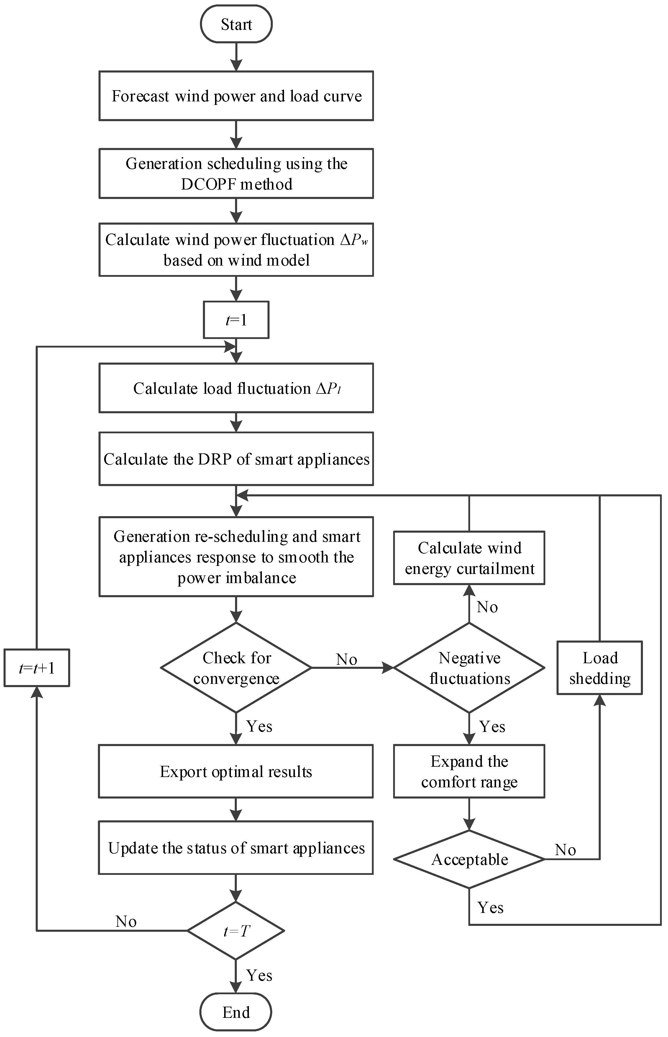
The way of determining the optimal combination of AGC units and DR reserve power for maximizing the wind accommodation is presented as the following flowchart (see Figure 3). First, the wind power and load curve are forecasted and the output power of thermal units is scheduled using the direct current optimal power flow (DCOPF) method in Matpower [30]. Based on the wind model described in Section 2, the wind power fluctuation is calculated. Considering the operating characteristics of smart appliances, including ACs, WHs, and EVs, it is obvious that their working status are the accumulated results of previous operation, and there is a load fluctuation calculated in Equation (22). The wind and load fluctuations result in the system imbalance, and the wind accommodation is maximized with the combination function of the supply-side and demand-side considering the constraints in Section 4.1.
When the AGC units regulating capability and DRP are not large enough to smooth the power imbalance, there would be wind energy curtailment with a negative fluctuation or load shedding with a positive fluctuation. In the condition of positive fluctuation, the comfort range is expanded to increase the DRP within the consumers’ acceptable limits.
5. Case Study
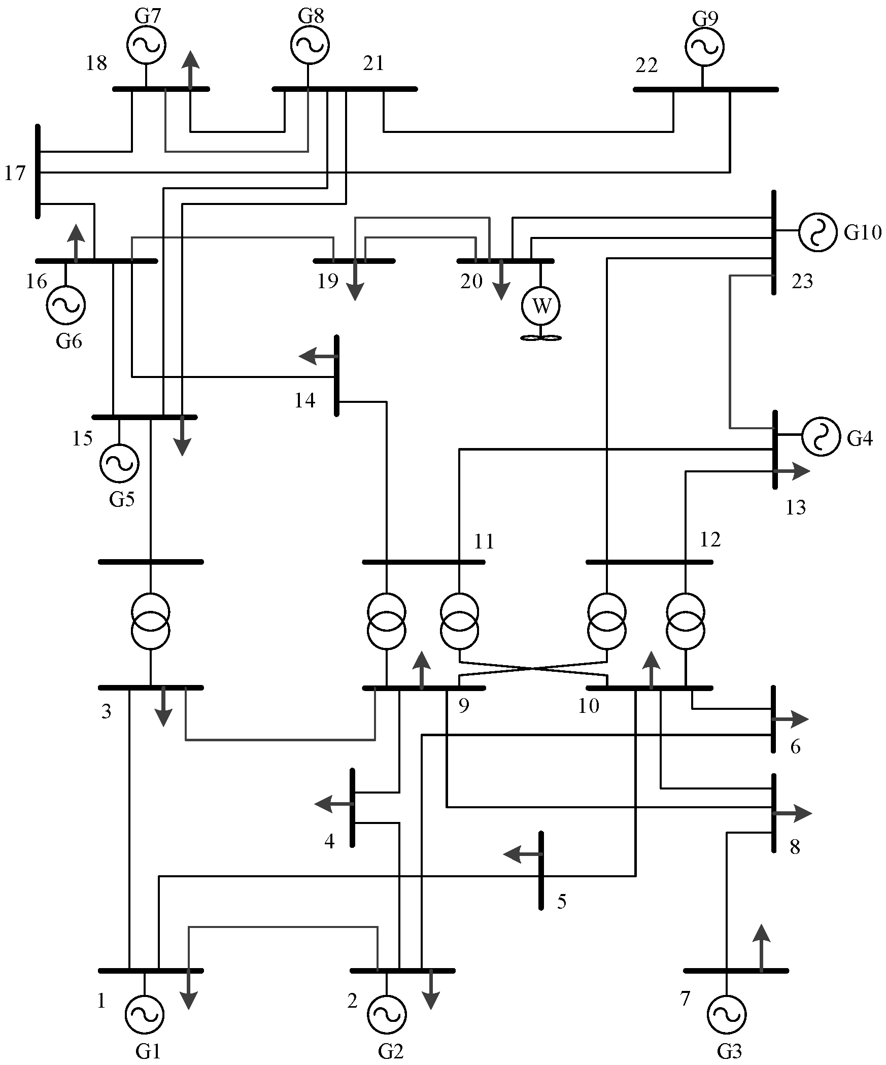
The proposed model was tested on a modified IEEE 24-node system over a daily time horizon whose data was taken from Reference [31]. The system comprises 34 transmission lines, illustrated in Figure 4. The wind farm is located at bus 20. The load profile used for testing was obtained as given in Figure 5. The 24-node system includes 17 loads. Both the nodal location of these loads and their contribution in percentage to the total system demand are listed in Table 1. It was assumed that there were smart appliances in 10 nodes, including nodes 3, 4, 5, 6, 8, 9, 10, 14, 19, and 20. The time interval was 1 min.
An ensemble of wind farms with a total installed capacity of = 600 MW is connected to the base system as an example. The wind forecast power data is taken based on [32], and its forecasting error is distributed normally as shown in Section 2. Figure 6 shows the actual and prediction wind power.
To showcase the benefits offered from the proposed methodology, four distinct case studies were conducted as follows, in which the wind installed capacity was 600 MW and the DR percentage was 15%. The operator maximizes the wind accommodation for which, in Case 1, generating units provide energy and reserve and there is no DR participation to absorb as much wind power, but in Case 2, in addition to generators, smart houses can also participate in balancing the wind prediction error. The generator ramp constraint is not considered in Case 3, and the power flow transmission constraint is not taken into account in Case 4 in the condition of a wind percentage of 20% and DR percentage of 15%. The simulations were conducted in Matpower and Matlab [33]. The observations are reported in the following subsection.
5.1. Simulation Results
Figure 7 shows the generator’s ability to smooth the wind fluctuation in Case 1. It is clear that the generator capability deviated from the imbalanced power. The generator capability varies owing to the wind fluctuation, negative or positive, and the different generator output for every time interval. The generator capability was smaller than the imbalanced power most of the time, which indicates that the AGC units cannot smooth the wind prediction error, and hence the curtailment of renewable generation, or even load shedding, are inevitable during large fluctuations. The estimated load shedding was 130.77 kWh. It can be obviously anticipated that additional balancing reserves are required in order to accommodate the wind output as much as possible.
As discussed earlier, the smart appliances—including AC, WH, and EV loads—are highly flexible, and the shifting of the smart appliances in time to smooth the wind power fluctuation will bring greater benefits. The questions of how the smart appliances respond and how much DRP supports the balancing of wind power forecasting error are now explored.
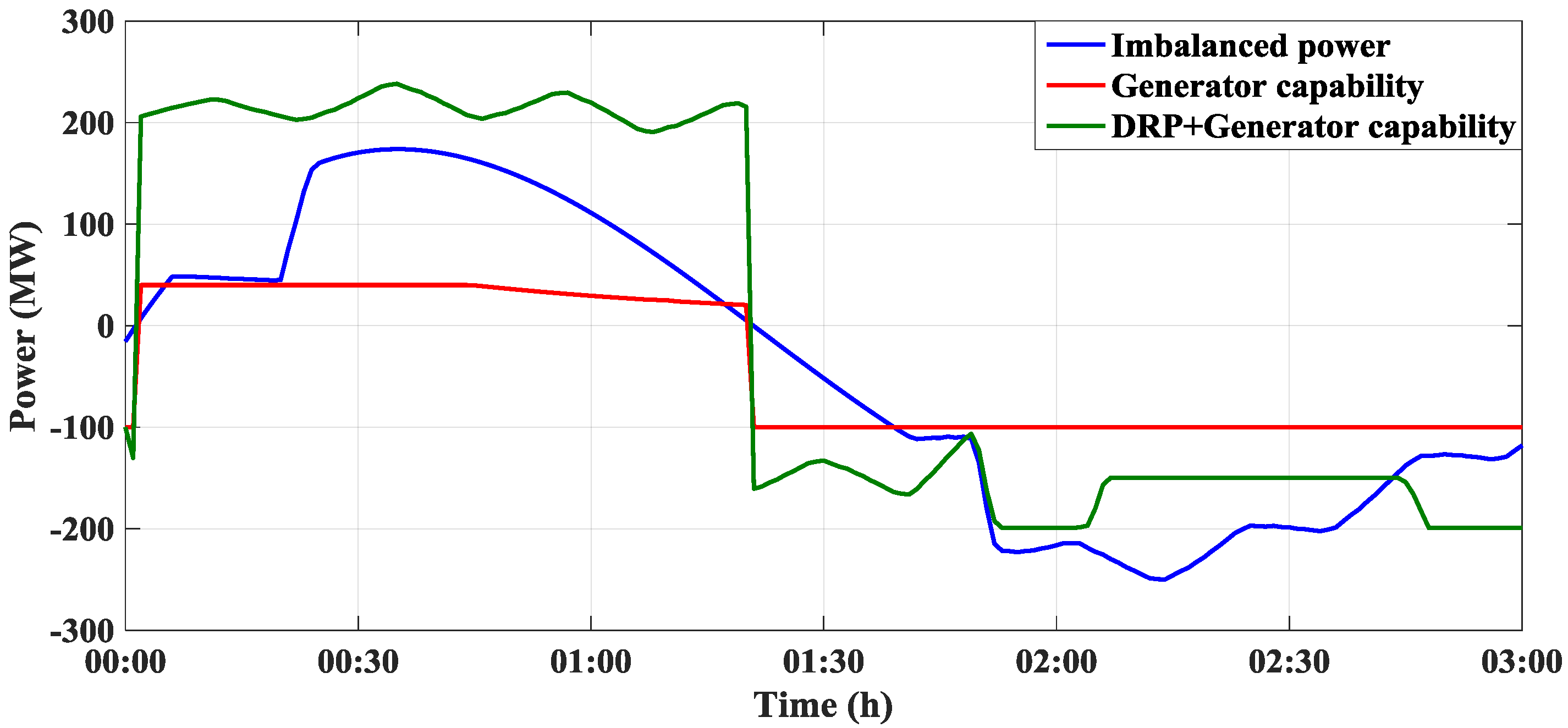
Figure 8 indicates the DRP and AGC unit capabilities and the unbalanced power. The red line represents the AGC unit capability, which is assumed negative when it provides reserve, and vice versa. The green line expresses the summation of DRP and AGC unit capability. The DRP is unlocked thanks to the domestic thermal storages that enable load shifting in order to smooth the wind forecast error. It is worth stating that the customers’ comfort—including the temperature preferences, travel distance ,and charging times—are respected at all times. However, as has been discussed in an earlier part of this paper, the DR strategy is not restricted to some specific method. The DR strategy could affect the following DRP, which varies at different time intervals. The DRP may not likely be large enough to smooth the wind forecast error. This phenomenon is observed during 01:50–02:44 a.m. The load-supply matching is disturbed because of large wind forecast error and little DRP. Consequently, the utilization of wind power could be enhanced if the system had more allowed DRP. It is worth revealing that the mismatching, wind power curtailment, and load shedding are a result of large fluctuations and DRP uncertainty.
Figure 9 shows the smart appliance results with and without the proposed method. In the process of optimization, the smart appliances provide up and down reserve based on the time-varying DR potential. It is obvious from the upper figure that the smart appliance power before DR is different from the power with no DR, which means the DR potential under these two conditions are also different. The difference between smart appliance power after DR and before DR is within the DR potential value. When the DR potential is not sufficient with negative unbalanced power, some other loads would be shed, like the green line of the lower figure.
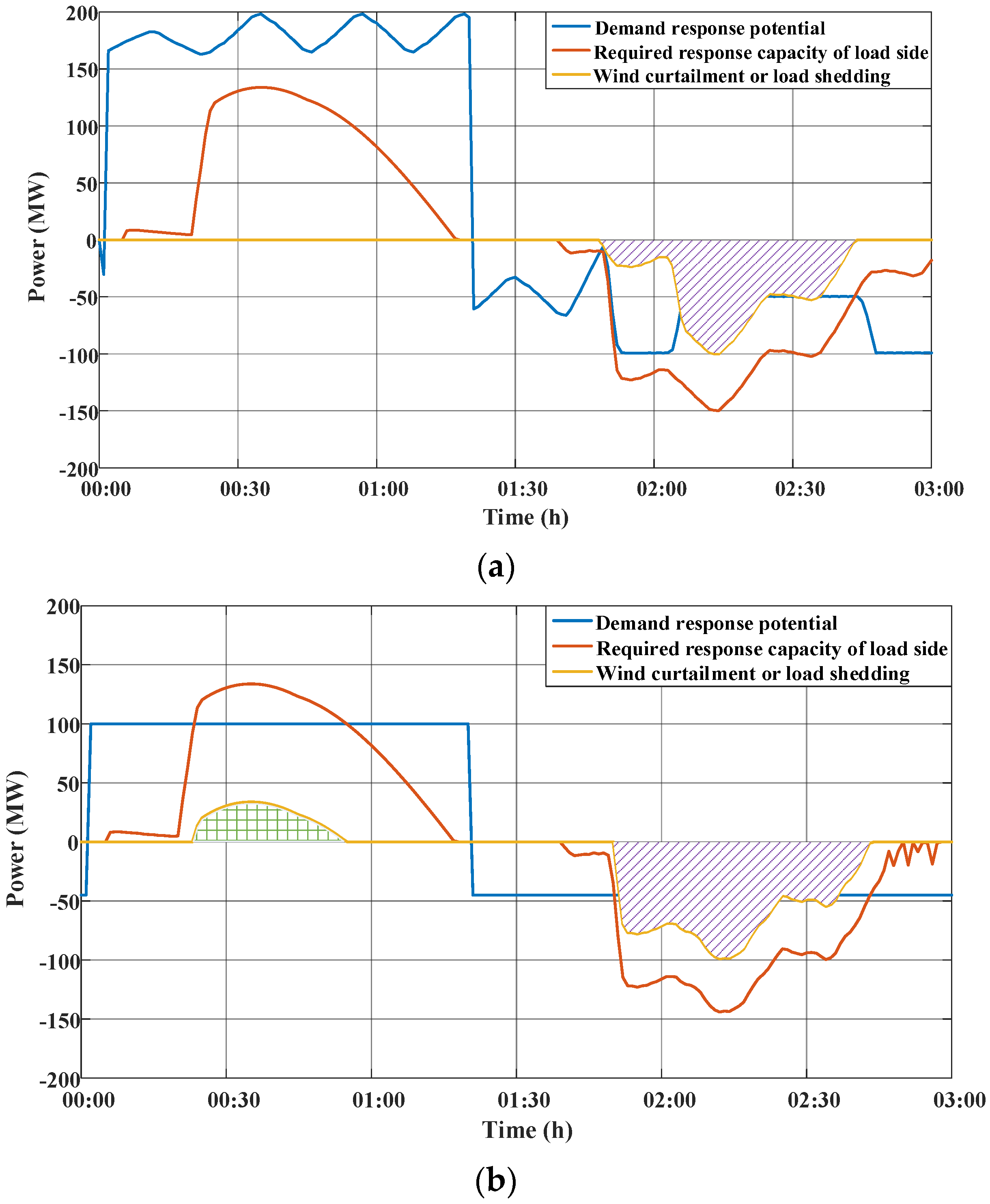
The conventional DRP is calculated in advance, such that the DRP is constant. It is assumed that the upward DRP is 100 MW and the downward DRP is 45 MW. Figure 10 shows the comparative results between the proposed time-varying DRP and constant DRP. During 00:00–01:20 a.m., the total fluctuation is positive and the smart appliances respond to the increment signal. The lower figure depicts that the green shadow is the wind curtailment energy because the DRP is lower than the required response capacity of the load side. During 01:29–03:00 a.m., the total fluctuation is negative and the smart appliances respond to the reduction signal. The purple shadow is the load shedding energy. The amount of load shedding is greater with constant DRP than with the time-varying DRP.
When the wind forecast error is large, there should be DR participation because of the AGC units’ output restrict. If the generator ramp constraint is not considered, the AGC units can provide an adequate up and down reserve, which is not correct in reality. The results are indicated in Figure 11 compared with taking the ramp constraint into account.
After the wind accommodation is maximized with the combination of generators and smart appliances, the line power varies and may be beyond the limit. Table 2 shows the line active power without and with power flow transmission constraint at a given time. As shown in Figure 4, the branches 15–21, 18–21, 19–20, and 20–23 are double circuit lines. Therefore, their power limit and line active power are depicted as the corresponding parameter of the single line multiplied by two in Table 2. It can be seen that the active power of branch 14–16 shown in red frame exceeds the power limit in the condition of not considering the power flow transmission constraint.
The wind forecasting power and its error are 225.78 MW and −74.06 MW, respectively. The load forecasting power is 2545.45 MW. Table 3 shows the results with and without considering power flow transmission constraint. In the condition of with power flow transmission constraint, even though the line power is lower because of less load fluctuation, the smart appliances respond to the 4.06 MW load reduction signal in order to keep the line power within the limitation. The DR power is 0 without considering the power flow transmission constraint, in which the generator regulating capability is abundant to balance the fluctuation. Therefore, it is indispensable to consider the power flow transmission constraint in the process of optimizing the utilization of DR.
5.2. Wind and Smart House Penetration Level
In the basic simulation, it was supposed that the wind penetration percentage is 20% and the DR percentage is 15%. However, this may not be considerate in practice. Therefore, it is imperative to evaluate the impact of the wind penetration and smart houses enrollment level on the wind energy curtailment and load shedding. There are several assumptions for the wind percentage and DR percentage, which are shown as follows:
- (1)
- The wind penetration percentage equals the installed capacity of wind generation divided by the maximum total load.
- (2)
- The maximum power of a house in one day is 12 kW. The total number of houses is maximum total load divided by 12 kW.
- (3)
- All the smart houses contain three kinds of smart appliances, whose working parameters are indicated in Table 4.
- (4)
- The DR percentage is a number of smart houses expressed as a fraction of all houses.
Quite a few simulations have been performed by changing the wind and smart house penetration percentages. Based on the mentioned assumptions, the simulation data are shown as follows: If the maximum load is 2658 MW, then the installed wind capacities are approximately 265 MW, 530 MW, and 795 MW when the wind penetration percentages are 10%, 20%, and 30%, respectively, and the total number of smart houses in the studied system are roughly 11,050, 22,100, 33,150, and 44,200 when the DR percentages are 5%, 10%, 15%, and 20%.
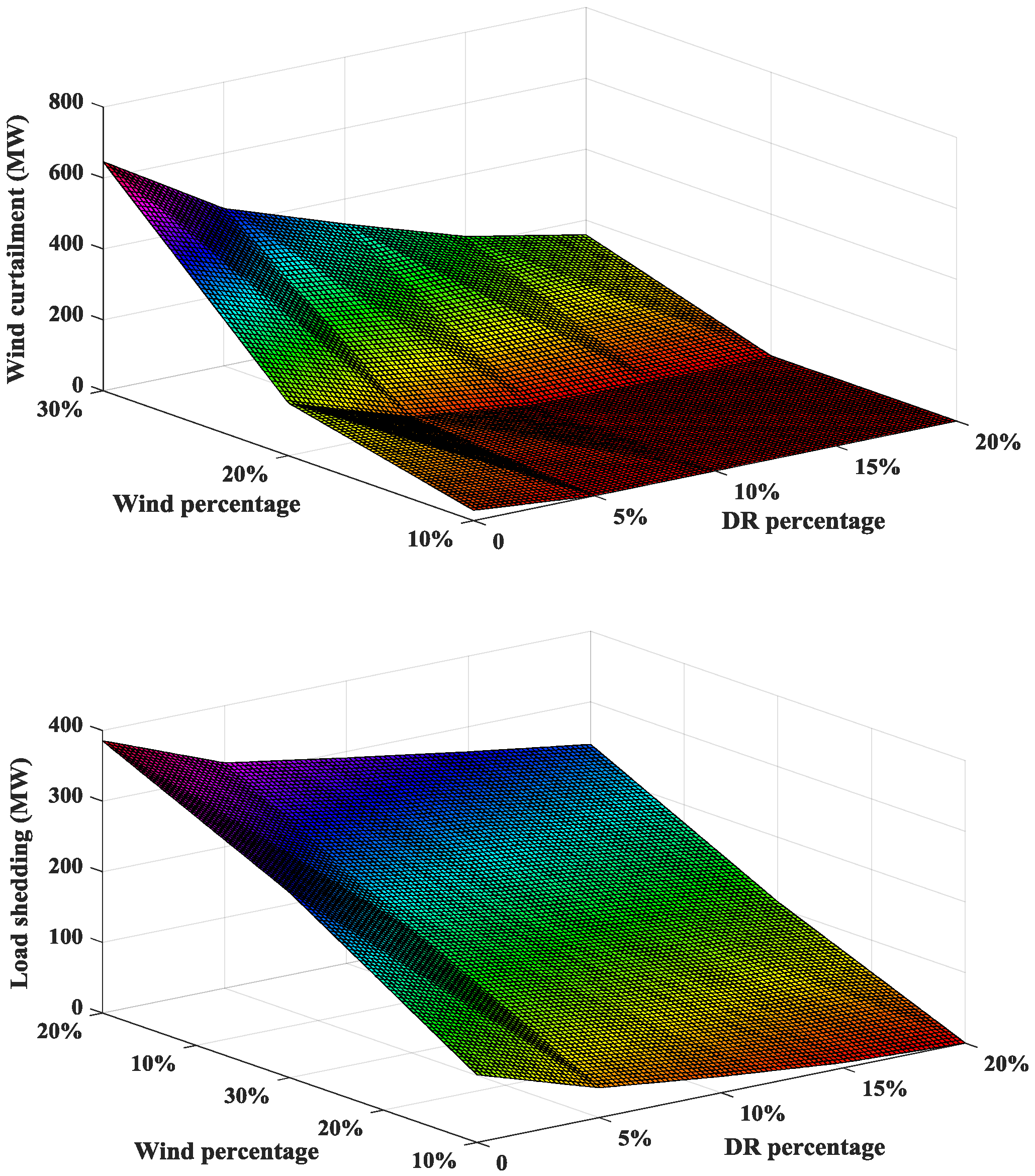
The wind generation curtailment and load shedding are listed in Table 5 with different wind and DR percentages. Here, the comfort ranges of smart appliances are fixed. The wind energy curtailment decreases from 645.71 MW to 158.4 MW when the wind percentage is 30% and the DR percentage is from 0% to 20%. From the relation between DR percentage and wind energy curtailment with 10% and 20% wind percentage, it is easily derived that the wind curtailment could reduce to 0 with the DR percentage increasing as the wind percentage is 30%. There is a similar variation tendency for load shedding as the wind and DR percentage change.
This result will serve as a strong motivation to provide an incentive to distribution companies to utilize more DR. Figure 12 shows the impact of DR and wind percentage on wind curtailment and load shedding using the interpolation method based on the information in Table 5.
Figure 12 shows the correlation among wind percentage, DR percentage, and wind power curtailment/load shedding. The wind curtailment or load shedding reduce as the number of enrolled smart houses increases and wind power decreases.
6. Conclusions
This paper proposes a real-time optimal method to mitigate the WPFE impacts by the coordination of AGC units and residential DR. Consequently, a comprehensive model is proposed that enables AGC units and DR to function to mitigate the effect of wind power forecasting error. The model is applicable no matter what kind of DR load control method is used. Since the wind forecasting error may not be offset by employing conventional generation resources and further leads to wind curtailment or load shedding, the smart appliances’ loads—including AC, WH, and EV—are applied in the optimal scheduling to alleviate the WPFE impacts. Furthermore, the quantifying DR potential method is presented considering consumers’ comfort and smart appliances’ dynamic characteristics, which reflect the time-scale variability of DRP. To ensure the safety and stability of the power system, the generator ramp constraint and power flow transmission constraint are necessarily considered. The proposed method could reveal the correlation among the wind percentage, DR percentage, and wind curtailment/load shedding, which can provide ancillary decisions under diverse operational conditions. The obtained results confirmed that the collaboration of residential DR and AGC units can improve the ability of wind accommodation and reduce load shedding. Other DR categories, such as the industrial DR and commercial DR, should be considered in future studies.
Acknowledgments
This work is supported by the National Natural Science Foundation of China (grant no. 51577030).
Author Contributions
Jia Ning, Yi Tang and Bingtuan Gao contributed in developing the ideas of this research. Jia Ning performed this research. All the authors read and approved the final manuscript.
Conflicts of Interest
The authors declare no conflict of interest.
Abbreviations
| AC | Air Conditioner |
| AGC | Automatic Generation Control |
| DCOPF | Direct Current Optimal Power Flow |
| DO | Dispatching Order |
| DR | Demand Response |
| DRP | Demand Response Potential |
| EV | Electric Vehicle |
| EWH | Electric Water Heater |
| SOC | State-of-Charge |
| RTCO | Real Time Control Order |
| WH | Water Heater |
| WPFE | Wind Power Forecasting Error |
References
- Menemenlis, N.; Huneault, M.; Robitaille, A. Computation of dynamic operating balancing reserve for wind power integration for the time-horizon 1–48 hours. IEEE Trans. Sustain. Energy 2012, 3, 692–702. [Google Scholar] [CrossRef]
- Tamrakar, U.; Shrestha, D.; Maharjan, M.; Bhattarai, B.P.; Hansen, T.M.; Tonkoski, R. Virtual inertia: Current trends and future directions. Appl. Sci. 2017, 7, 654. [Google Scholar] [CrossRef]
- Zhang, D.; Eseye, A.T.; Zhang, J.; Li, H. Short-term wind power forecasting using a double-stage hierarchical ANFIS approach for energy management in microgrids. Prot. Control Mod. Power Syst. 2017, 2. [Google Scholar] [CrossRef]
- Zhang, N.; Kang, C.; Xia, Q.; Liang, J. Modeling conditional forecast error for wind power in generation scheduling. IEEE Trans Power Syst. 2014, 29, 1316–1324. [Google Scholar] [CrossRef]
- Mudumbai, R.; Dasgupta, S.; Cho, B.B. Distributed control for optimal economic dispatch of a network of heterogeneous power generators. IEEE Trans. Power Syst. 2012, 27, 1750–1760. [Google Scholar] [CrossRef]
- Banakar, H.; Luo, C.; Ooi, B.T. Impacts of wind power minute-to-minute variations on power system operation. IEEE Trans. Power Syst. 2008, 23, 150–160. [Google Scholar] [CrossRef]
- Chen, Q.; Zhao, X.; Gan, D. Active-reactive scheduling of active distribution system considering interactive load and battery storage. Prot. Control Mod. Power Syst. 2017, 2. [Google Scholar] [CrossRef]
- Khodayar, M.E.; Shahidehpour, M.; Wu, L. Enhancing the dispatchability of variable wind generation by coordination with pumped-storage hydro units in stochastic power systems. IEEE Trans. Power Syst. 2013, 28, 2808–2818. [Google Scholar] [CrossRef]
- Greenblatt, J.B.; Succar, S.; Denkenberger, D.C.; Williams, R.H.; Socolow, R.H. Baseload wind energy: Modeling the competition between gas turbines and compressed air energy storage for supplemental generation. Energy Policy 2007, 35, 1474–1492. [Google Scholar] [CrossRef]
- Yener, B.; Taşcıkaraoğlu, A.; Erdinç, O.; Baysal, M.; Catalão, J.P.S. Design and implementation of an interactive interface for demand response and home energy management applications. Appl. Sci. 2017, 7, 641. [Google Scholar]
- Jovanovic, R.; Bousselham, A.; Bayram, I.S. Residential demand response scheduling with considering of consumer preferences. Appl. Sci. 2016, 6, 16. [Google Scholar]
- Hamilton, K.; Gulhar, N. Taking demand response to the next level. IEEE Power Energy Mag. 2010, 8, 60–65. [Google Scholar] [CrossRef]
- Praktiknjo, A. The value of lost load for sectoral load shedding measures: The German case with 51 sectors. Energies 2016, 9, 116. [Google Scholar] [CrossRef] [Green Version]
- Erdinç, O.; Tascıkaraoglu, A.; Paterakis, N.G.; Catalão, J.P.S.; Eren, Y. End-user comfort oriented day-ahead planning for responsive residential HVAC demand aggregation considering weather forecasts. IEEE Trans. Smart Grid 2017, 8, 362–372. [Google Scholar] [CrossRef]
- Luo, F.; Zhao, J.; Dong, Z.; Tong, X.; Chen, Y.; Yang, H.; Zhang, H. Optimal dispatch of air conditioner loads in southern China region by direct load control. IEEE Trans. Smart Grid 2016, 7, 439–450. [Google Scholar] [CrossRef]
- Shad, M.; Momeni, A.; Errouissi, R.; Diduch, C.P.; Kaye, M.E.; Chang, L. Identification and estimation for electric water heaters in direct load control programs. IEEE Trans. Smart Grid 2017, 8, 947–955. [Google Scholar] [CrossRef]
- Papavasiliou, A.; Oren, S.S. A stochastic unit commitment model for integrating renewable supply and demand response. In Proceedings of the IEEE Power and Energy Society General Meeting, San Diego, CA, USA, 22–26 July 2012. [Google Scholar]
- Aghaei, J.; Barani, M.; Shafie-khah, M.; Sánchez de la Nieta, A.A.; Catalão, J.P.S. Risk-constrained offering strategy for aggregated hybrid power plant including wind power producer and demand response provider. IEEE Trans. Sustain. Energy 2016, 7, 513–525. [Google Scholar] [CrossRef]
- Pourmousavi, S.A.; Patrick, S.N.; Nehriri, M.H. Real-time demand response through aggregate electric water heaters for load shifting and balancing wind generation. IEEE Trans. Smart Grid 2014, 5, 769–778. [Google Scholar] [CrossRef]
- Çiçek, N.; Deliç, H. Demand response management for smart grids with wind power. IEEE Trans. Sustain. Energy 2015, 6, 625–634. [Google Scholar] [CrossRef]
- Ali, M.; Degefa, M.Z.; Humayun, M.; Safdarian, A.; Lehtonen, M. Increased utilization of wind generation by coordinating the demand response and real-time thermal rating. IEEE Trans. Power Syst. 2016, 31, 3737–3746. [Google Scholar] [CrossRef]
- Ortega-Vazquez, M.A.; Kirschen, D.S. Estimating the spinning reserve requirements in systems with significant wind power generation penetration. IEEE Trans. Power Syst. 2009, 24, 114–124. [Google Scholar] [CrossRef]
- Shao, S. An Approach to Demand Response for Alleviating Power System Stress Conditions Due to Electric Vehicle Penetration. Ph.D. Dissertation, Virginia Polytechnic Institute and State University, Arlington, VA, USA, 2011. [Google Scholar]
- Yao, L.; Lim, W.; Tsai, T. A real-time charging scheme for demand response in electric vehicle parking station. IEEE Trans. Smart Grid 2017, 8, 52–62. [Google Scholar] [CrossRef]
- Wan, Z.; Zhang, J.; Zheng, Y. Aggregation model of air-conditioning load demand response to adapt the wind power integration. In Proceedings of the IEEE International Conference on Power and Renewable Energy, Shanghai, China, 21–23 October 2016. [Google Scholar]
- GridLAB-D/Code/[r5643]:trunk/residential/autotest/water_schedule.glm. Available online: https://sourceforge.net/p/gridlab-d/code/HEAD/tree/trunk/residential/autotest/water_schedule.glm (accessed on 3 July 2014).
- Santos, A.; McGuckin, N.; Nakamoto, H.Y.; Gay, D.; Liss, S. Summary of Travel Trends: 2009 National Household Travel Survey; Rep. FHWA-PL-11022; U.S. Department of Transportation Federal Highway Administration: Washington, DC, USA, 2011.
- Ning, J.; Tang, Y.; Gao, W. A hierarchical charging strategy for electric vehicles considering the users’ habits and intentions. In Proceedings of the IEEE Power and Energy Society General Meeting, Denver, CO, USA, 26–30 July 2015. [Google Scholar]
- Ning, J.; Tang, Y.; Chen, Q.; Wang, J.; Zhou, J.; Gao, B. A bi-level coordinated optimization strategy for smart appliances considering online demand response potential. Energies 2017, 10, 525. [Google Scholar] [CrossRef]
- MATPOWER-A MATLAB Power System Simulation Package. Available online: http://www.pserc.cornell.edu/matpower/ (accessed on 16 December 2016).
- Conejo, A.J.; Carrion, M.; Morales, J.M. Appendix B 24-node system data. In Decision Making Under Uncertainty in Electricity Markets; Springer Science + Business Media: New York, NY, USA, 2010; pp. 479–485. [Google Scholar]
- Falsafi, H.; Zakariazadeh, A.; Jadid, S. The role of demand response in single and multi-objective wind-thermal generation scheduling: A stochastic programming. Energy 2014, 64, 853–867. [Google Scholar] [CrossRef]
- MathWorks, MATLAB. Available online: https://cn.mathworks.com/products/matlab.html (accessed on 12 June 2017).
Figure 1.
Demand response potential (DRP) of air conditioner (AC) and water heater (WH) in response to a load reduction signal.
Figure 1.
Demand response potential (DRP) of air conditioner (AC) and water heater (WH) in response to a load reduction signal.
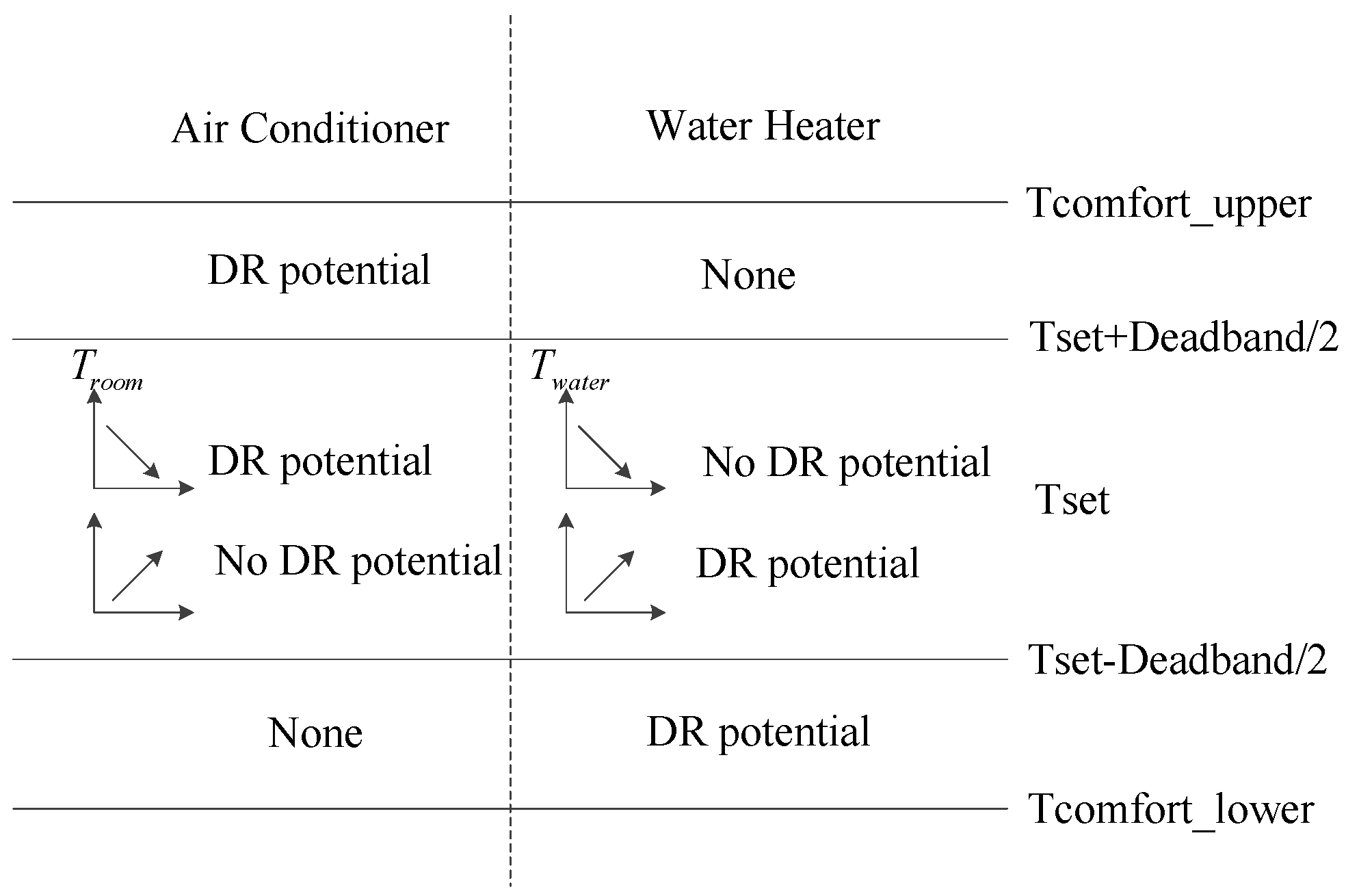
Figure 2.
Schematic diagram of coordinated real-time control of DR and automatic generation control (AGC) units. DO: dispatching order; RTCO: real-time control order; WPFE: wind power forecasting error.
Figure 2.
Schematic diagram of coordinated real-time control of DR and automatic generation control (AGC) units. DO: dispatching order; RTCO: real-time control order; WPFE: wind power forecasting error.
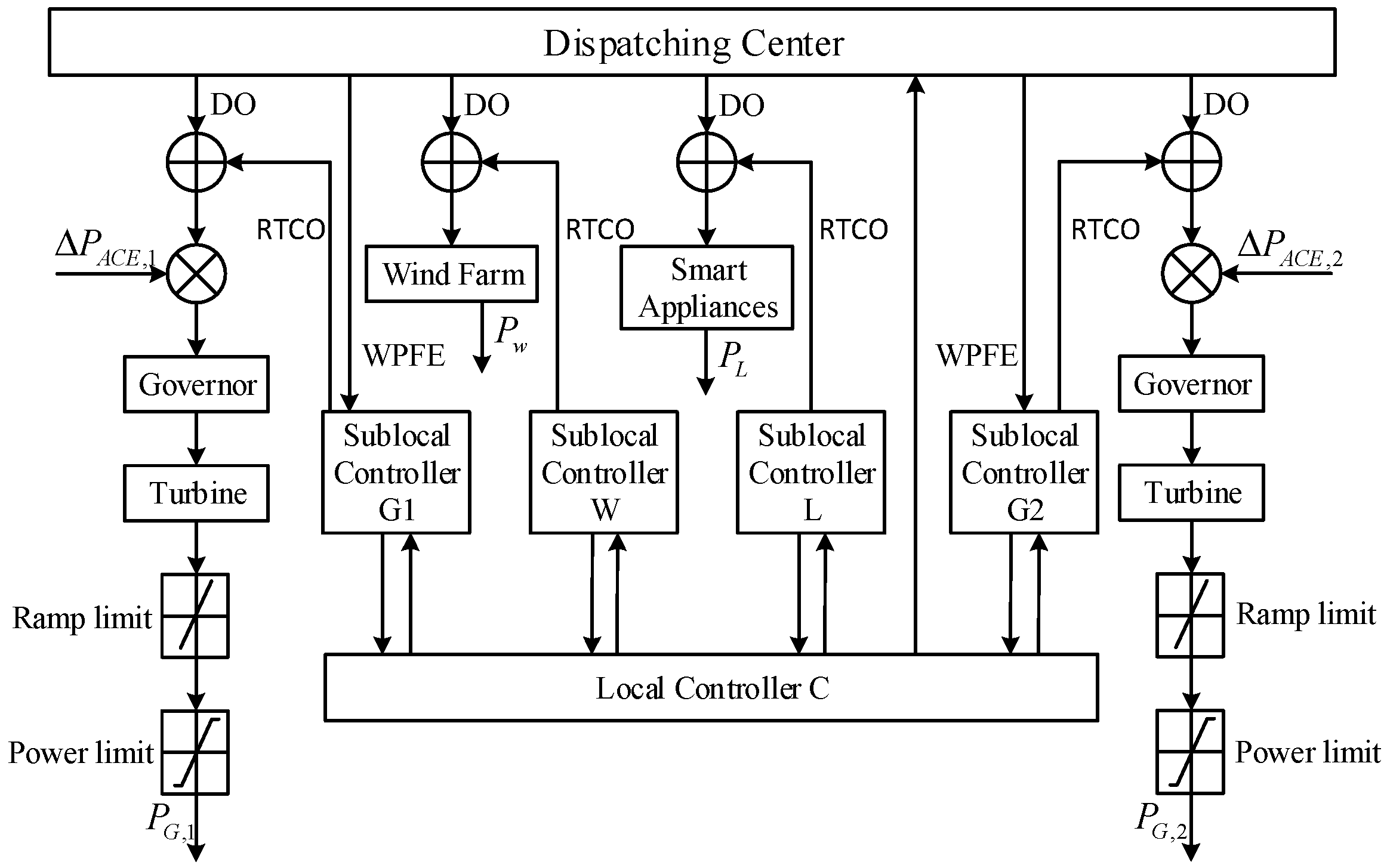
Figure 3.
Solution method’s flowchart. DCOPF: direct current optimal power flow.

Figure 4.
The modified IEEE 24-node system.

Figure 5.
The daily load profile.
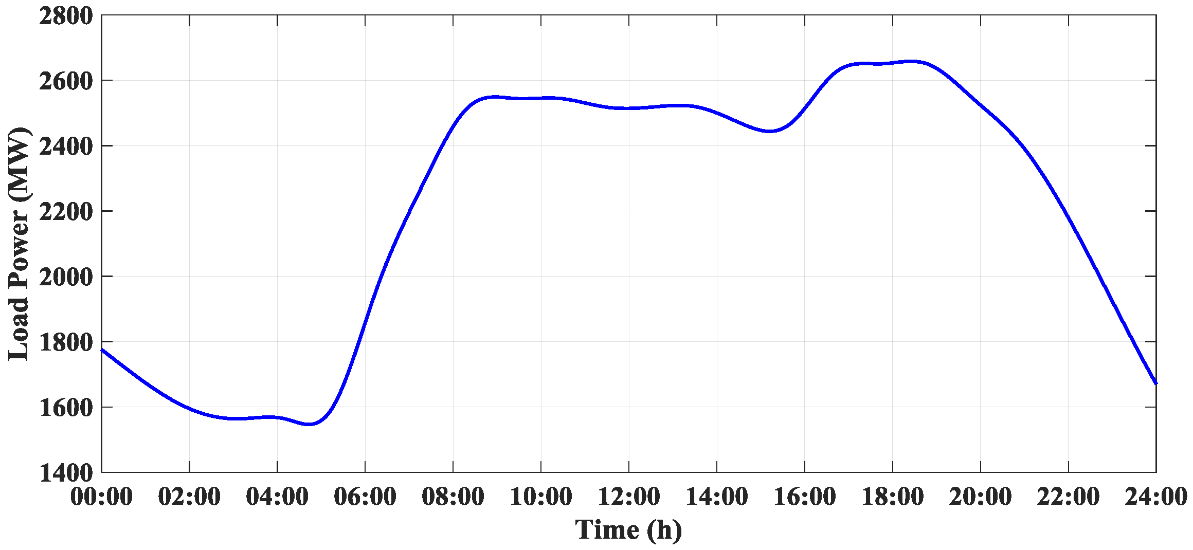
Figure 6.
The actual and prediction wind power.
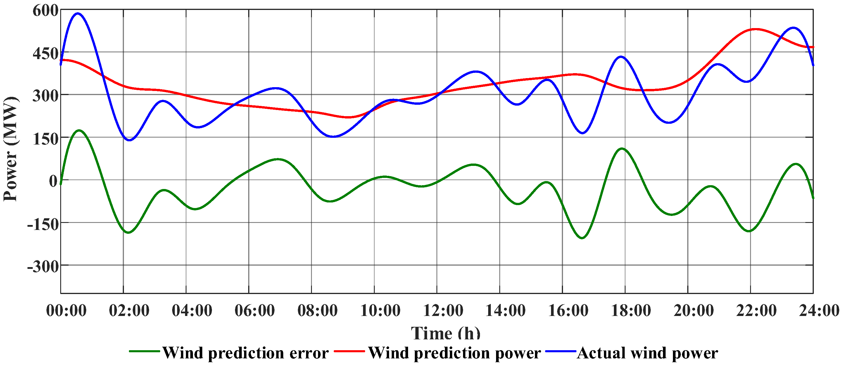
Figure 7.
The system operational power without DR.
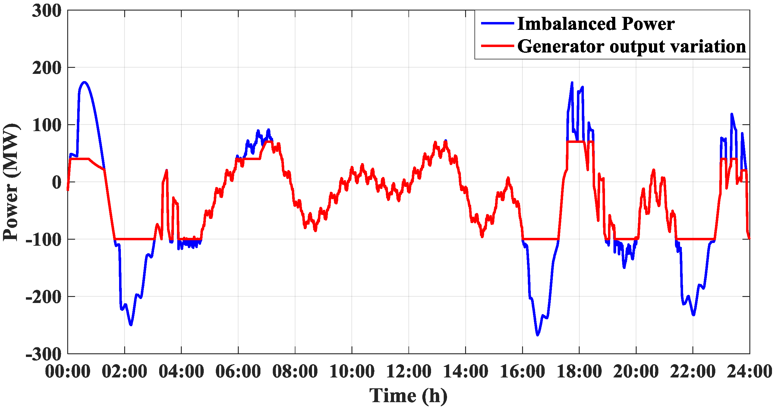
Figure 8.
DRP and AGC unit capabilities and wind prediction error power.

Figure 9.
The smart appliance results with and without the proposed method.
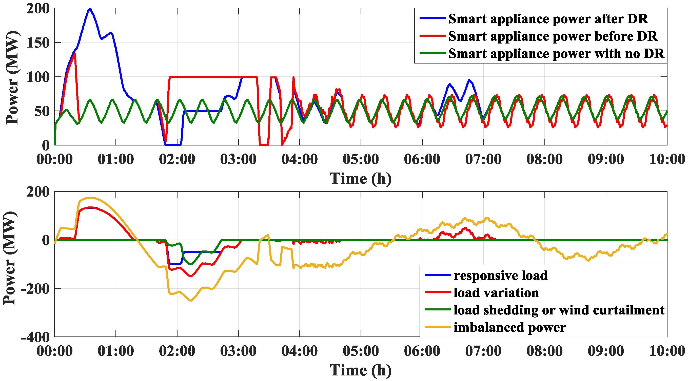
Figure 10.
Comparative results: (a) load response results with time-varying DRP; and (b) load response results with constant DRP.
Figure 10.
Comparative results: (a) load response results with time-varying DRP; and (b) load response results with constant DRP.

Figure 11.
Results of DR and generator output variation without/with the ramp constraint.

Figure 12.
Impact of DR and wind percentage on wind curtailment and load shedding.

Table 1.
The 24-node system: node location and distribution of the total system load.
| Load | Node | Percentage | Load | Node | Percentage |
|---|---|---|---|---|---|
| 1 | 1 | 3.8 | 10 | 10 | 6.8 |
| 2 | 2 | 3.4 | 11 | 13 | 9.3 |
| 3 | 3 | 6.3 | 12 | 14 | 6.8 |
| 4 | 4 | 2.6 | 13 | 15 | 11.1 |
| 5 | 5 | 2.5 | 14 | 16 | 3.5 |
| 6 | 6 | 4.8 | 15 | 18 | 11.7 |
| 7 | 7 | 4.4 | 16 | 19 | 6.4 |
| 8 | 8 | 6.0 | 17 | 20 | 4.5 |
| 9 | 9 | 6.1 |
Table 2.
Line power without/with transmission constraint.
| Branch | Power Limit (MW) | Line Power w/o Transmission Constraint (MW) | Line Power with Transmission Constraint (MW) |
|---|---|---|---|
| 1–2 | 140 | 21.88 | 21.45 |
| 1–3 | 140 | −58.96 | −58.04 |
| 1–5 | 140 | 12.76 | 12.26 |
| 2–4 | 140 | −6.72 | −6.96 |
| 2–6 | 140 | 14.46 | 14.27 |
| 3–9 | 140 | 35.81 | 34.98 |
| 3–24 | 408 | −257.13 | −253.79 |
| 4–9 | 140 | −73.72 | −72.44 |
| 5–10 | 140 | −51.92 | −51.02 |
| 6–10 | 140 | −108.88 | −107.55 |
| 7–8 | 140 | −27.00 | −27.00 |
| 8–9 | 140 | −104.33 | −103.39 |
| 8–10 | 140 | −75.95 | −75.37 |
| 9–11 | 408 | −145.52 | −143.76 |
| 9–12 | 408 | −153.56 | −152.42 |
| 10–11 | 408 | −201.36 | −198.90 |
| 10–12 | 408 | −209.41 | −207.56 |
| 11–13 | 400 | −115.47 | −115.36 |
| 11–14 | 400 | −231.40 | −227.30 |
| 12–13 | 400 | −101.29 | −100.09 |
| 12–23 | 400 | −261.67 | −259.90 |
| 13–23 | 400 | −236.49 | −235.17 |
| 14–16 | 400 | −405.49 | −400 |
| 15–16 | 400 | 88.09 | 86.98 |
| 15–21 | 400 × 2 | −237.51 × 2 | −235.28 × 2 |
| 15–24 | 400 | 257.13 | 253.79 |
| 16–17 | 400 | −347.17 | −342.54 |
| 16–19 | 400 | 77.30 | 71.17 |
| 17–18 | 400 | −205.58 | −200.99 |
| 17–22 | 400 | −141.59 | −141.55 |
| 18–21 | 400 × 2 | −46.70 × 2 | −48.94 × 2 |
| 19–20 | 400 × 2 | −43.92 × 2 | −46.20 × 2 |
| 20–23 | 400 × 2 | −25.60 × 2 | −27.15 × 2 |
| 21–22 | 400 | −158.41 | −158.45 |
Table 3.
Results without/with transmission constraint.
| Transmission Constraint | Generator Power (MW) | Load Fluctuation (MW) | DR Power (MW) |
|---|---|---|---|
| with | 2390.58 | 0.92 | −4.06 |
| without | 2405.53 | 11.81 | 0 |
Table 4.
Parameters of smart appliances. EV: electric vehicle.
| Parameter | Value | Unit |
|---|---|---|
| Cooling set point | 22 | °C |
| AC thermostat dead band | 1 | °C |
| AC power consumption | 3 | kW |
| WH temperature set point | 47 | °C |
| WH thermostat dead band | 6 | °C |
| WH power consumption | 4 | kW |
| EV power consumption | 3.3 | kW |
| EV efficiency of driving | 3.846 | mile/kWh |
| EV charging efficiency | 0.9 | - |
Table 5.
Wind energy curtailment and load shedding energy with different wind and DR percentage.
| Wind Percentage | DR Percentage | Wind Energy Curtailment (MWh) | Load Shedding (MWh) |
|---|---|---|---|
| 10% | 0% | 29.50 | 95.85 |
| 5% | 0 | 42.30 | |
| 10% | 0 | 23.21 | |
| 15% | 0 | 7.52 | |
| 20% | 0 | 0.29 | |
| 20% | 0% | 148.74 | 262.28 |
| 5% | 41.87 | 175.20 | |
| 10% | 3.26 | 148.36 | |
| 15% | 0 | 130.77 | |
| 20% | 0 | 108.21 | |
| 30% | 0% | 645.71 | 385.38 |
| 5% | 443.40 | 318.88 | |
| 10% | 329.52 | 290.79 | |
| 15% | 224.10 | 264.24 | |
| 20% | 158.40 | 239.70 |
© 2017 by the authors. Licensee MDPI, Basel, Switzerland. This article is an open access article distributed under the terms and conditions of the Creative Commons Attribution (CC BY) license (http://creativecommons.org/licenses/by/4.0/).
Share and Cite
MDPI and ACS Style
Ning, J.; Tang, Y.; Gao, B. A Time-Varying Potential-Based Demand Response Method for Mitigating the Impacts of Wind Power Forecasting Errors. Appl. Sci. 2017, 7, 1132. https://doi.org/10.3390/app7111132
AMA Style
Ning J, Tang Y, Gao B. A Time-Varying Potential-Based Demand Response Method for Mitigating the Impacts of Wind Power Forecasting Errors. Applied Sciences. 2017; 7(11):1132. https://doi.org/10.3390/app7111132
Chicago/Turabian StyleNing, Jia, Yi Tang, and Bingtuan Gao. 2017. "A Time-Varying Potential-Based Demand Response Method for Mitigating the Impacts of Wind Power Forecasting Errors" Applied Sciences 7, no. 11: 1132. https://doi.org/10.3390/app7111132
Note that from the first issue of 2016, this journal uses article numbers instead of page numbers. See further details here.