Incipient Fault Feature Extraction of Rolling Bearings Using Autocorrelation Function Impulse Harmonic to Noise Ratio Index Based SVD and Teager Energy Operator


Abstract
:1. Introduction
2. Theory Background
2.1. The Fundamental of SVD Denoising Method
2.2. Autocorrelation Function Impulse Harmonic to Noise Ratio Index
2.3. Teager Energy Operator
3. The Proposed Method
4. Simulation Analysis
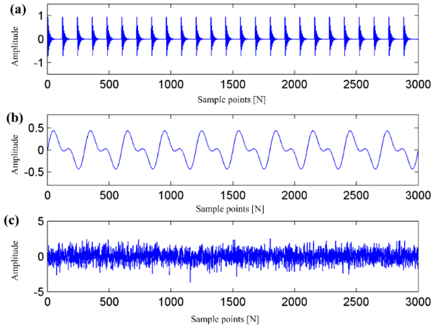
4.1. The Stimulated Signal
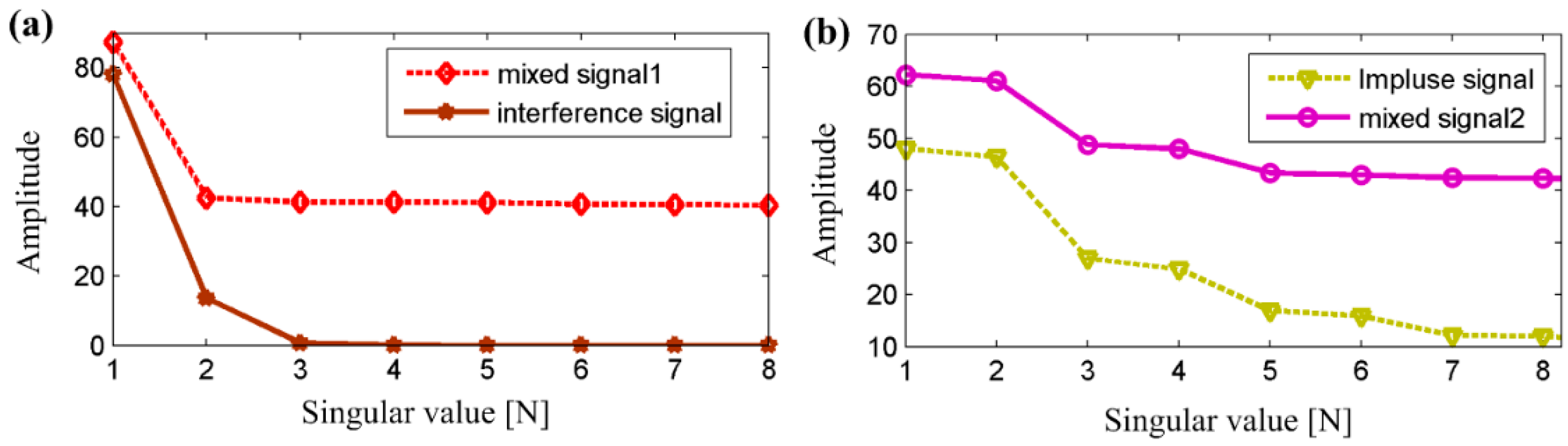
4.2. The Performance Analysis of the Proposed Method
5. Experiment Results
6. Conclusions
- (1)
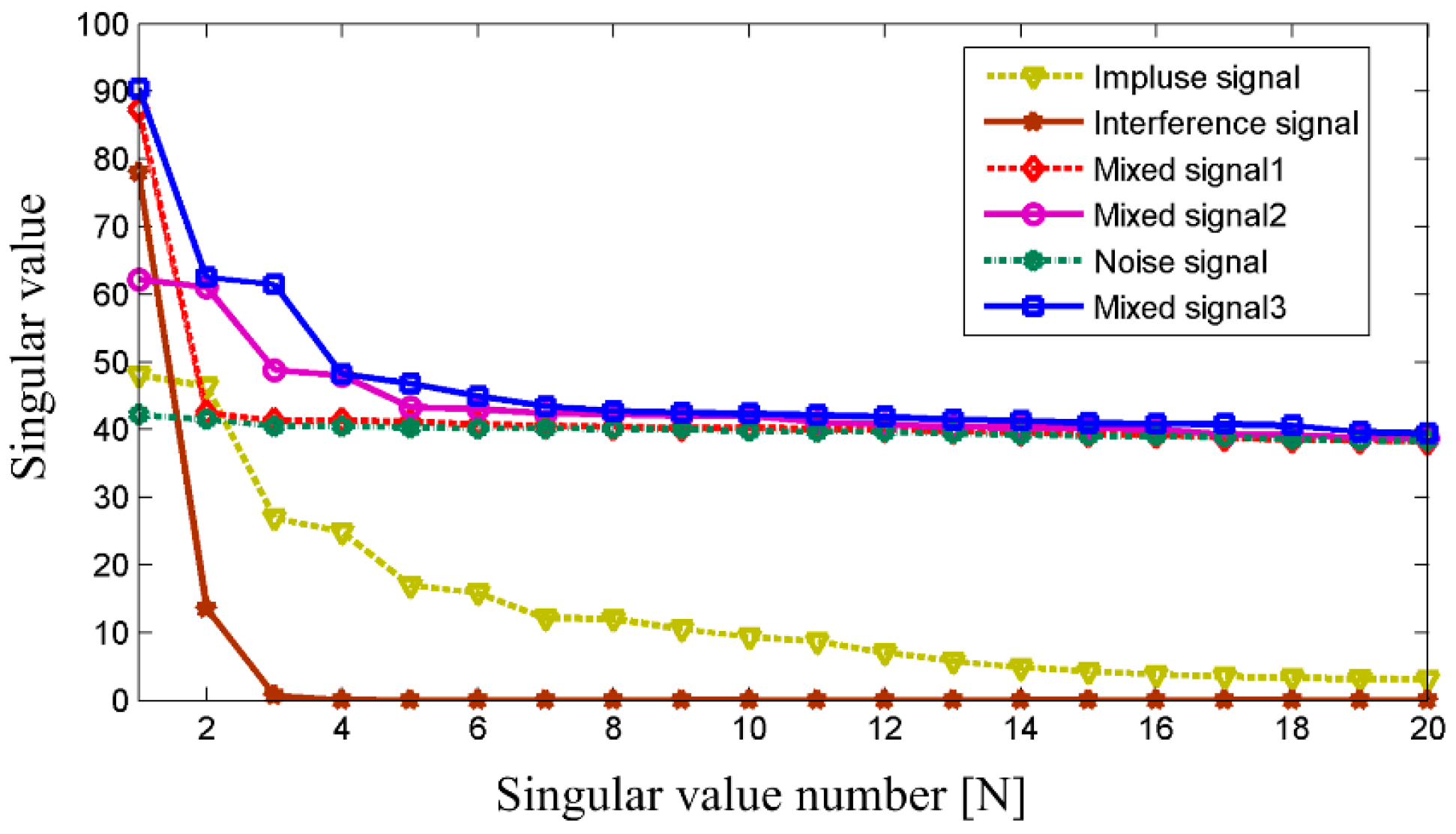
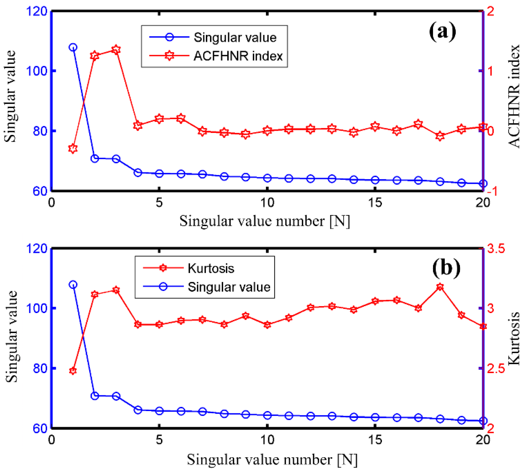
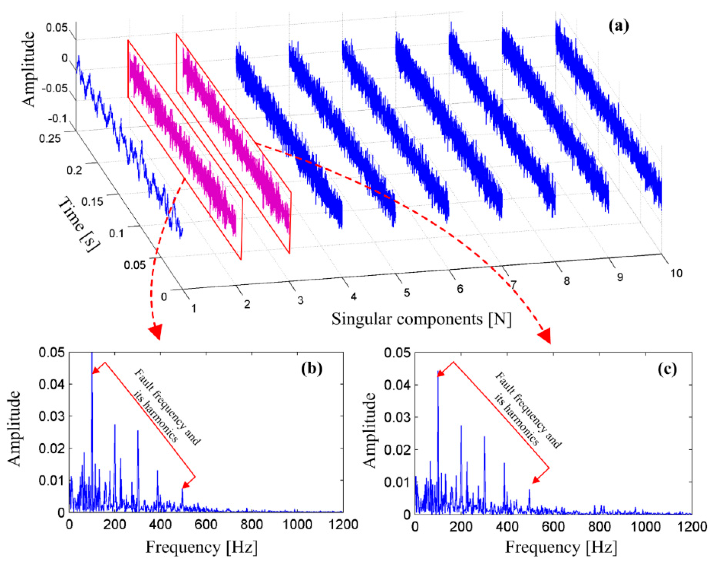
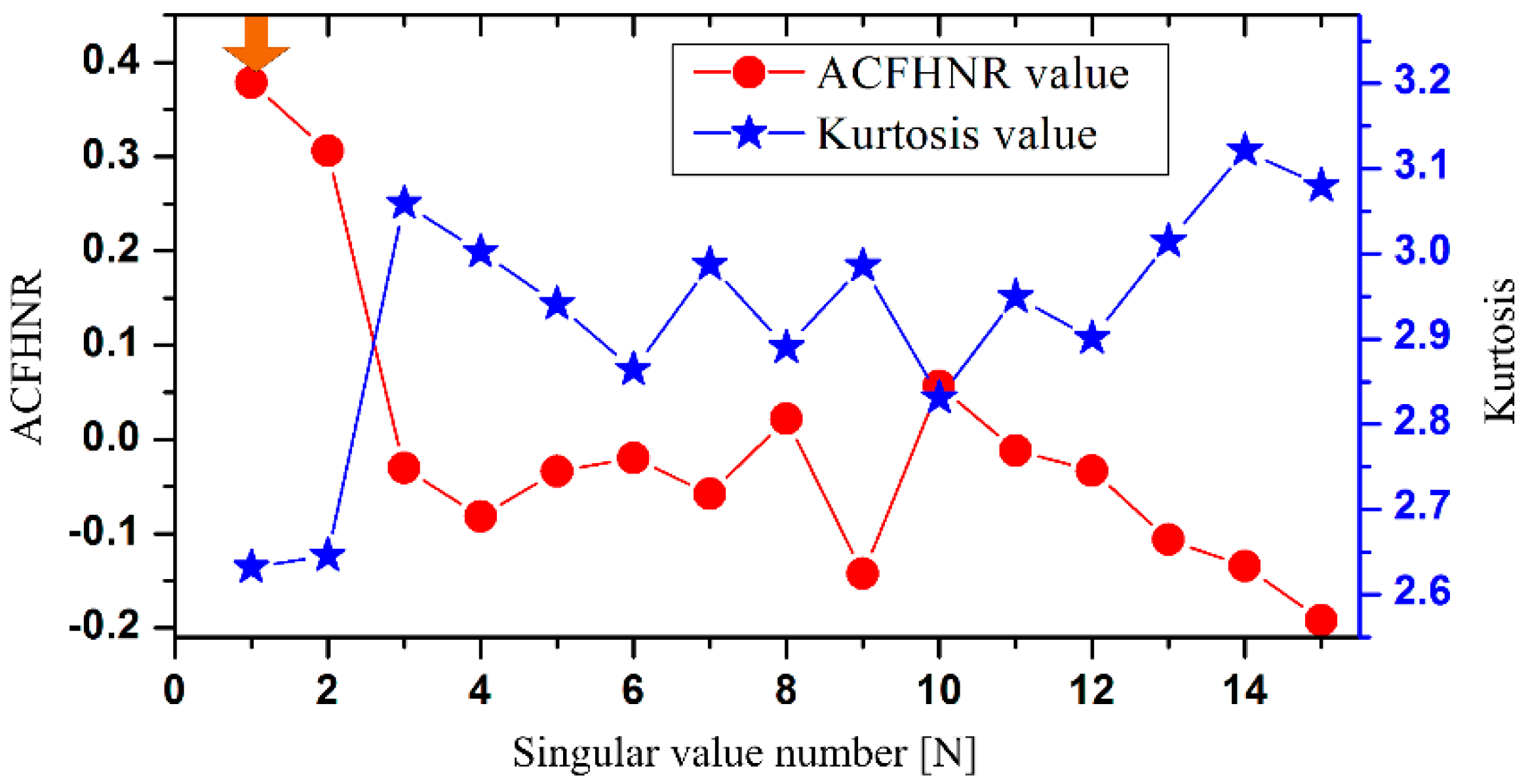
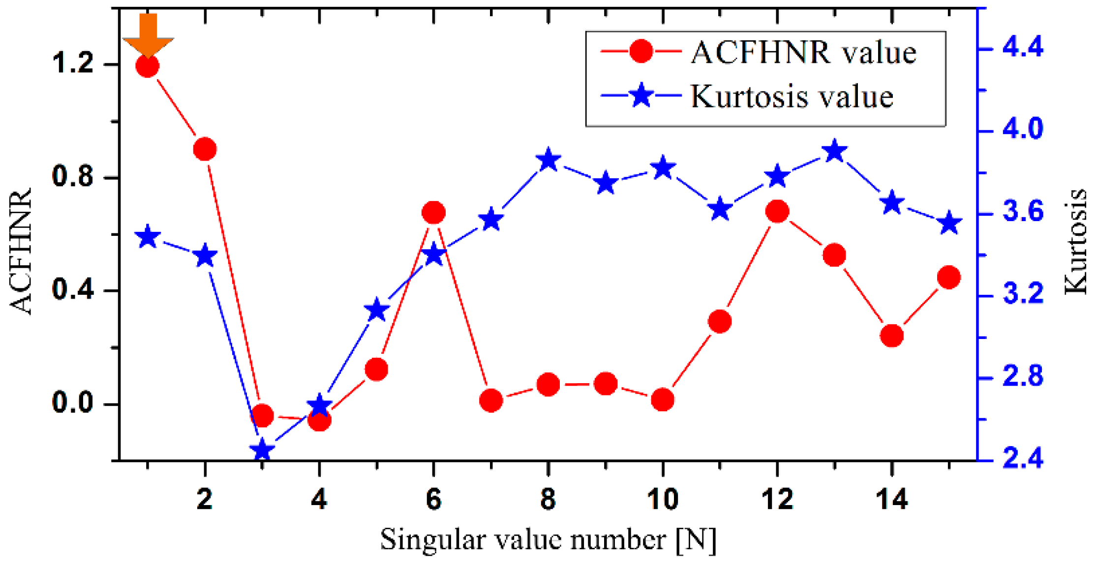
- Compared with the kurtosis index, the sensitive singular components obtained by the SVD method can be clearly identified with the proposed ACFHNR index. Moreover, the incipient fault features of the vibration signal from the rolling element bearings can be detected by the proposed ACFHNR-SVD method combined with Teager energy operator method. They are proved by the simulation and experimental results.
- (2)
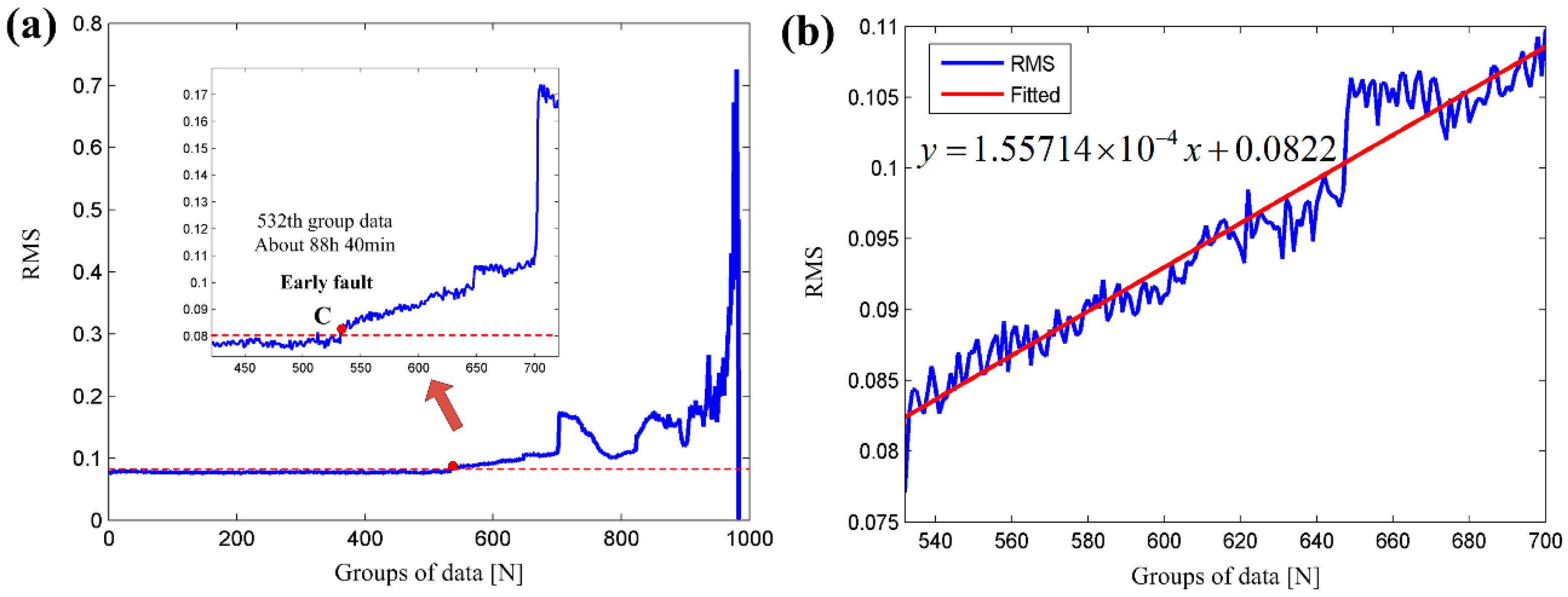
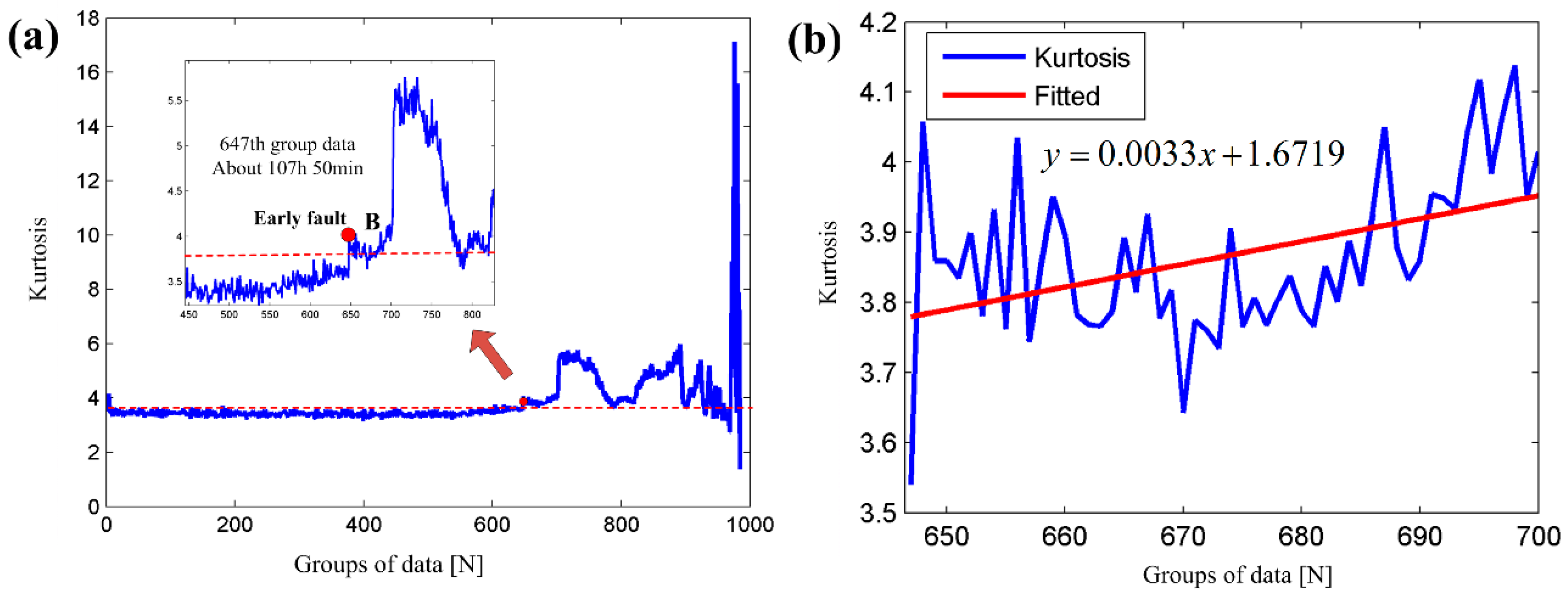
- The ACFHNR index is able to detect faults earlier than the kurtosis index. Moreover, compared with kurtosis and RMS indexes, the sensitivity value of the ACFHNR index is the largest in the incipient fault stage, demonstrating its superiority over the traditional RMS and kurtosis indexes for detecting the early fault features of the vibration signal. This is proved by the full life cycle of the bearing degradation data.
Acknowledgments
Author Contributions
Conflicts of Interest
References
- Qiao, Z.; Pan, Z. SVD principle analysis and fault diagnosis for bearings based on the correlation coefficient. Meas. Sci. Technol. 2015, 26, 085014. [Google Scholar] [CrossRef]
- Li, H.; Lian, X.; Guo, C.; Zhao, P. Investigation on early fault classification for rolling element bearing based on the optimal frequency band determination. J. Intell. Manuf. 2015, 26, 189–198. [Google Scholar] [CrossRef]
- Lei, Y.; Lin, J.; He, Z.; Zuo, M.J. A review on empirical mode decomposition in fault diagnosis of rotating machinery. Mech. Syst. Signal Process. 2013, 35, 108–126. [Google Scholar] [CrossRef]
- Aydin, I.; Karakose, M.; Akin, E. Combined intelligent methods based on wireless sensor networks for condition monitoring and fault diagnosis. J. Intell. Manuf. 2015, 26, 717–729. [Google Scholar] [CrossRef]
- Golafshan, R.; Sanliturk, K.Y. SVD and Hankel matrix based de-noising approach for ball bearing fault detection and its assessment using artificial faults. Mech. Syst. Signal Process. 2016, 70, 36–50. [Google Scholar] [CrossRef]
- Wang, J.; Qiao, L.; Ye, Y.; Chen, Y.Q. Fractional envelope analysis for rolling element bearing weak fault feature extraction. IEEE/CAA J. Autom. Sin. 2017, 4, 353–360. [Google Scholar] [CrossRef]
- Georgoulas, G.; Loutas, T.; Stylios, C.D.; Kostopoulos, V. Bearing fault detection based on hybrid ensemble detector and empirical mode decomposition. Mech. Syst. Signal Process. 2013, 41, 510–525. [Google Scholar] [CrossRef]
- Zhao, M.; Lin, J.; Xu, X.; Lei, Y. Tacholess envelope order analysis and its application to fault detection of rolling element bearings with varying speeds. Sensors 2013, 13, 10856–10875. [Google Scholar] [CrossRef] [PubMed]
- Chandra, N.H.; Sekhar, A.S. Fault detection in rotor bearing systems using time frequency techniques. Mech. Syst. Signal Process. 2016, 72–73, 105–133. [Google Scholar] [CrossRef]
- Zhang, Z.; Wang, Y.; Wang, K. Fault diagnosis and prognosis using wavelet packet decomposition, Fourier transform and artificial neural network. J. Intell. Manuf. 2013, 24, 1213–1227. [Google Scholar] [CrossRef]
- Jin, S.; Lee, S.K. Bearing fault detection utilizing group delay and the Hilbert-Huang transform. J. Mech. Sci. Technol. 2017, 31, 1089–1096. [Google Scholar] [CrossRef]
- Zheng, K.; Zhang, Y.; Zhao, C.; Li, T. Fault Diagnosis for Supporting Rollers of the Rotary Kiln Using the Dynamic Model and Empirical Mode Decomposition. Mechanics 2016, 22, 198–205. [Google Scholar] [CrossRef]
- Singh, J.; Darpe, A.K.; Singh, S.P. Bearing damage assessment using Jensen-Rényi Divergence based on EEMD. Mech. Syst. Signal Process. 2017, 87, 307–339. [Google Scholar] [CrossRef]
- Xu, T.; Yin, Z.; Cai, D.; Zheng, D. Fault diagnosis for rotating machinery based on Local Mean Decomposition morphology filtering and Least Square Support Vector Machine. J. Intell. Fuzzy Syst. 2017, 32, 2061–2070. [Google Scholar] [CrossRef]
- Zhao, M.; Jia, X. A novel strategy for signal denoising using reweighted SVD and its applications to weak fault feature enhancement of rotating machinery. Mech. Syst. Signal Process. 2017, 94, 129–147. [Google Scholar] [CrossRef]
- Jiang, H.; Chen, J.; Dong, G.; Liu, T.; Chen, G. Study on Hankel matrix-based SVD and its application in rolling element bearing fault diagnosis. Mech. Syst. Signal Process. 2015, 52, 338–359. [Google Scholar] [CrossRef]
- Muruganatham, B.; Sanjith, M.A.; Krishnakumar, B.; Murty, S.S. Roller element bearing fault diagnosis using singular spectrum analysis. Mech. Syst. Signal Process. 2013, 35, 150–166. [Google Scholar] [CrossRef]
- Hernandez-Vargas, M.; Cabal-Yepez, E.; Garcia-Perez, A. Real-time SVD-based detection of multiple combined faults in induction motors. Comput. Electr. Eng. 2014, 40, 2193–2203. [Google Scholar] [CrossRef]
- Cong, F.; Zhong, W.; Tong, S.; Tang, N.; Chen, J. Research of singular value decomposition based on slip matrix for rolling bearing fault diagnosis. J. Sound Vib. 2015, 344, 447–463. [Google Scholar] [CrossRef]
- Zhao, X.; Ye, B. Selection of effective singular values using difference spectrum and its application to fault diagnosis of headstock. Mech. Syst. Signal Process. 2011, 25, 1617–1631. [Google Scholar] [CrossRef]
- Han, T.; Jiang, D.; Wang, N. The fault feature extraction of rolling bearing based on EMD and difference spectrum of singular value. Shock Vib. 2016, 2016, 5957179. [Google Scholar] [CrossRef]
- Wang, H.; Chen, J.; Dong, G. Feature extraction of rolling bearing’s early weak fault based on EEMD and tunable Q-factor wavelet transform. Mech. Syst. Signal Process 2014, 48, 103–119. [Google Scholar] [CrossRef]
- Xu, X.; Zhao, M.; Lin, J.; Lei, Y. Envelope harmonic-to-noise ratio for periodic impulses detection and its application to bearing diagnosis. Measurement 2016, 91, 385–397. [Google Scholar] [CrossRef]
- Jiang, Y.; Tang, B.; Qin, Y.; Liu, W. Feature extraction method of wind turbine based on adaptive Morlet wavelet and SVD. Renew. Energy 2011, 36, 2146–2153. [Google Scholar] [CrossRef]
- Wang, Z.; Lu, C.; Wang, Z.; Liu, H.; Fan, H. Fault diagnosis and health assessment for bearings using the Mahalanobis-Taguchi system based on EMD-SVD. Trans. Inst. Meas. Control 2013, 35, 798–807. [Google Scholar] [CrossRef]
- Liu, Y.; Yu, Z.; Zeng, M.; Zhang, Y. LLE for submersible plunger pump fault diagnosis via joint wavelet and SVD approach. Neurocomputing 2016, 185, 202–211. [Google Scholar] [CrossRef]
- Xu, J.; Tong, S.; Cong, F.; Chen, J. Slip Hankel matrix series-based singular value decomposition and its application for fault feature extraction. IET Sci. Meas. Technol. 2017, 11, 464–472. [Google Scholar] [CrossRef]
- Ding, J. Detection of the dynamic imbalance with cardan shaft in high-speed train applying eemd-hankel-svd. J. Mech. Eng. 2015, 51, 143. [Google Scholar] [CrossRef]
- Li, Y.; Liang, X.; Xu, M.; Huang, W. Early fault feature extraction of rolling bearing based on ICD and tunable Q-factor wavelet transform. Mech. Syst. Signal Process. 2017, 86, 204–223. [Google Scholar] [CrossRef]
- Zhao, S.; Liang, L.; Xu, G.; Wang, J.; Zhang, W. Quantitative diagnosis of a spall-like fault of a rolling element bearing by empirical mode decomposition and the approximate entropy method. Mech. Syst. Signal Process 2013, 40, 154–177. [Google Scholar] [CrossRef]
- Imaouchen, Y.; Kedadouche, M.; Alkama, R.; Thomas, M. A Frequency-Weighted Energy Operator and complementary ensemble empirical mode decomposition for bearing fault detection. Mech. Syst. Signal Process. 2017, 82, 103–116. [Google Scholar] [CrossRef]
- Sun, P.; Liao, Y.; Lin, J. The shock pulse index and its application in the fault diagnosis of rolling element bearings. Sensors 2017, 17, 535. [Google Scholar] [CrossRef] [PubMed]
- Ming, A.B.; Qin, Z.Y.; Zhang, W.; Chu, F.L. Spectrum auto-correlation analysis and its application to fault diagnosis of rolling element bearings. Mech. Syst. Signal Process 2013, 41, 141–154. [Google Scholar] [CrossRef]
- Zhao, H.; Li, L. Fault diagnosis of wind turbine bearing based on variational mode decomposition and Teager energy operator. IET Renew. Power Gen. 2016, 11, 453–460. [Google Scholar] [CrossRef]
- Rodriguez, P.H.; Alonso, J.B.; Ferrer, M.A.; Travieso, C.M. Application of the Teager–Kaiser energy operator in bearing fault diagnosis. ISA Trans. 2013, 52, 278–284. [Google Scholar] [CrossRef] [PubMed]
- Pineda-Sanchez, M.; Puche-Panadero, R.; Riera-Guasp, M.; Perez-Cruz, J.; Roger-Folch, J.; Pons-Llinares, J.; Antonino-Daviu, J.A. Application of the Teager–Kaiser energy operator to the fault diagnosis of induction motors. IEEE Trans. Energy Conver. 2013, 28, 1036–1044. [Google Scholar] [CrossRef]
- Lou, X.; Loparo, K.A. Bearing fault diagnosis based on wavelet transform and fuzzy inference. Mech. Syst. Signal Process 2004, 18, 1077–1095. [Google Scholar] [CrossRef]
- Lee, J.; Qiu, H.; Yu, G.; Lin, J. Bearing Data Set, IMS. In Rexnord Technical Services; NASA Ames Prognostics Data Repository; University of Cincinnati: Cincinnati, OH, USA, 2007. [Google Scholar]


| Input: Signal x(t), Prior fault frequency , Sampling frequency |
| Procedure: |
| 1. The signal x(t) is subjected to Hilbert transform |
| 2. Compute the and the Interval point * |
| 3. Compute the Autocorrelation function |
| 4. Set = 0, Compute , Set i |
| 5. Compute |
| Output: ACFHNR = |
| The Index | ACFHNR | Kurtosis | RMS |
|---|---|---|---|
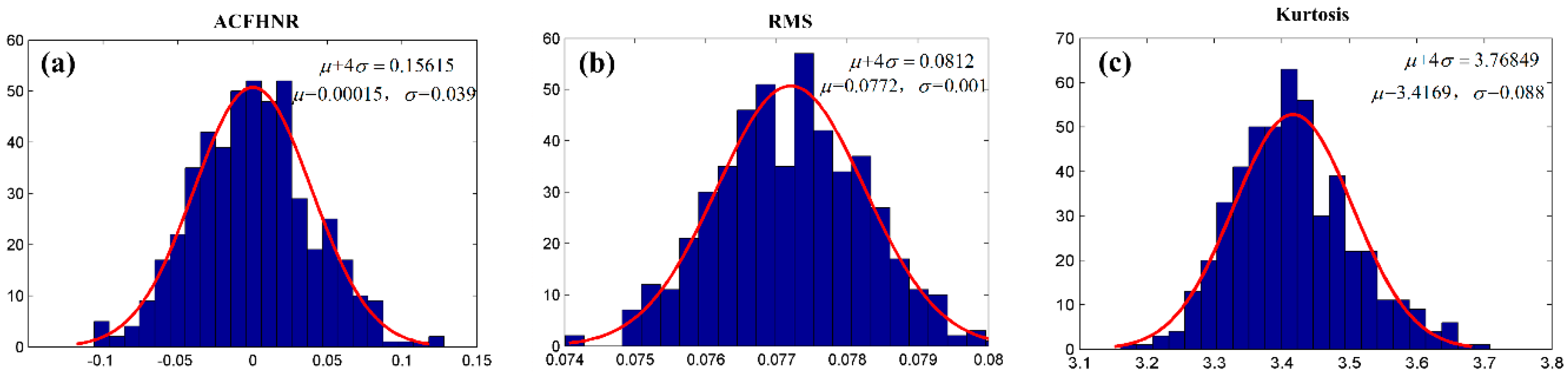
| Threshold value | 0.15615 | 3.76849 | 0.0812 |
| The Index | ACFHNR | Kurtosis | RMS |
|---|---|---|---|
| Sensitivity | 0.0261 | 0.0033 | 1.55714 × 10⁻⁴ |
© 2017 by the authors. Licensee MDPI, Basel, Switzerland. This article is an open access article distributed under the terms and conditions of the Creative Commons Attribution (CC BY) license (http://creativecommons.org/licenses/by/4.0/).
Share and Cite
Zheng, K.; Li, T.; Zhang, B.; Zhang, Y.; Luo, J.; Zhou, X. Incipient Fault Feature Extraction of Rolling Bearings Using Autocorrelation Function Impulse Harmonic to Noise Ratio Index Based SVD and Teager Energy Operator. Appl. Sci. 2017, 7, 1117. https://doi.org/10.3390/app7111117
Zheng K, Li T, Zhang B, Zhang Y, Luo J, Zhou X. Incipient Fault Feature Extraction of Rolling Bearings Using Autocorrelation Function Impulse Harmonic to Noise Ratio Index Based SVD and Teager Energy Operator. Applied Sciences. 2017; 7(11):1117. https://doi.org/10.3390/app7111117
Chicago/Turabian StyleZheng, Kai, Tianliang Li, Bin Zhang, Yi Zhang, Jiufei Luo, and Xiangyu Zhou. 2017. "Incipient Fault Feature Extraction of Rolling Bearings Using Autocorrelation Function Impulse Harmonic to Noise Ratio Index Based SVD and Teager Energy Operator" Applied Sciences 7, no. 11: 1117. https://doi.org/10.3390/app7111117