A Hospital Recommendation System Based on Patient Satisfaction Survey

Abstract

Surveys are used by hospitals to evaluate patient satisfaction and to improve general hospital operations. Collected satisfaction data is usually represented to the hospital administration by using statistical charts and graphs. Although such visualization is helpful, typically no deeper data analysis is performed to identify important factors which contribute to patient satisfaction. This work presents an unsupervised data-driven methodology for analyzing patient satisfaction survey data. The goal of the proposed exploratory data analysis is to identify patient communities with similar satisfaction levels and the major factors, which contribute to their satisfaction. This type of data analysis will help hospitals to pinpoint the prevalence of certain satisfaction factors in specific patient communities or clusters of individuals and to implement more proactive measures to improve patient experience and care. To this end, two layers of data analysis is performed. In the first layer, patients are clustered based on their responses to the survey questions. Each cluster is then labeled according to its salient features. In the second layer, the clusters of first layer are divided into sub-clusters based on patient demographic data. Associations are derived between the salient features of each cluster and its sub-clusters. Such associations are ranked and validated by using standard statistical tests. The associations derived by this methodology are turned into comments and recommendations for healthcare providers and patients. Having applied this method on patient and survey data of a hospital resulted in 19 recommendations where 10 of them were statistically significant with chi-square test’s p-value less than 0.5 and an odds ratio z-test’s p-value of more than 2 or less than −2. These associations not only are statistically significant but seems rational too.

1. Introduction

Patient satisfaction has been proven to be one of the most valid indicators of the quality of care. Analysis of patient satisfaction data is in demand by many health-care providers. Most health-care providers, from doctor’s offices to clinics and hospitals, collect patient satisfaction surveys to evaluate their various services and patient experience. This increasingly growing data is conventionally analyzed by statistical methods, such as analysis of variance (ANOVA) [1], simple regression, Fisher’s approach and extensions [2], Neyman’s approach to randomization-based inference [2], etc. Such methods typically approach the problem with a specific question in mind and find the relation between one or more independent variables and a dependent variable. For example, they compute the percentage of the patients that have rated each hospital’s services similarly or at most provide some correlations between specific groups of patients and their answers to a specific satisfaction question.

For improving patient satisfaction, issues of health care provided at the hospital level and the factors that originate those issues from patients’ point of view should be discovered. Therefore, survey data should be either manually analyzed by examining each possible pattern in the data set using conventional methods or an unsupervised methodology is needed to do the analysis with least amount of human interaction. Such methodology should get the satisfaction survey data, find patterns that are repeated among patients’ demographics and their satisfaction level in different fields, validate the patterns and compile them into a set of recommendations to help hospitals improve satisfaction within various patient communities.

To this end, a new hybrid methodology is proposed that differs from these conventional approaches in that it is not bound to a single outcome or dependent variable. The focus of this approach is to find patterns in patients’ responses to all satisfaction questions and relate them to patients’ demographics. The proposed methodology is focused on discovering issues of the health care provided at the hospital level and the factors that originate those issues from the patients’ point of view. This methodology is a hybrid unsupervised clustering-labeling method, which finds associations between various levels of patients’ satisfaction and demographics. The associations are validated by using standard statistical models and turned into useful recommendations for hospitals in order to improve patients’ experience, save cost, and build long-term patient loyalty. The methodology can be generalized to any complex multi-level survey analysis.

The article is organized into eight sections. The next section describes the standard survey instrument used for collecting patient satisfaction data. Section 3 reviews the literature on the analysis of hospital survey data as well as modern survey data analysis methods. The proposed methodology for the analysis of the survey data will be presented in Section 4. Section 5 reports on the experimental results of the analysis using the Hospital Consumer Assessment of Healthcare Providers and Systems (HCAHPS) dataset. The validation of the results of the analysis are discussed in Section 6. Section 7 explains how to convert the associations derived from the analysis into recommendations for healthcare providers. The last section draws a conclusion and future direction of this study.

2. Literature Review

This section describes the HCAHPS dataset and briefly reviews modern survey data analysis methods and their shortcomings in analyzing the HCAHPS dataset.

2.1. HCAHPS Hospital Survey Data

HCAHPS [3] is a standard survey instrument used by many hospitals to evaluate patients’ experience. This data is provided by the HCAHPS database, which is funded by U.S. agency for health care research. The centers for Medicaid and Medicare services use the scores from HCAHPS to reimburse hospitals for patient care. Providing a high quality care is directly related to a hospital’s revenue and many hospitals are looking for ways to improve patient experience and achieve a higher HCAHPS score.

Table 1. Satisfaction Questions Categories.

Section	Number of Question in Each Section	Number of Choices for Each Question
Care from Nurses	5	4
Care from Doctors	3	4
Hospital Environment	2	4
Experience in Hospital	5	4
When You Left	1	2
Overall Rating	1	2
	1	11

gives a brief description of the satisfaction questions on the HCAHPS survey instrument and the categories that they fall into. As shown in the table, the survey questions are divided into six sections where each section has a number of multiple choice questions. The number of choices for each question is also specified in Table 1. For instance, the section on “care from doctor” measures patient satisfaction with the care provided by doctor(s) using three questions about doctor’s respect, listening, and explaining. Each question has four choices (Never, Sometimes, Usually, and Always).

Table 2. Demographic Data Types.

Questions	Number of Choices
Age	-
Discharge Date	-
State	44
Racial Category	6
Overall Health	5
Education	6
Ethnicity	5
Patient-Filled Race	5
Patient’s Language	3
Gender	2
Principal Reason	3
Admission Source	10
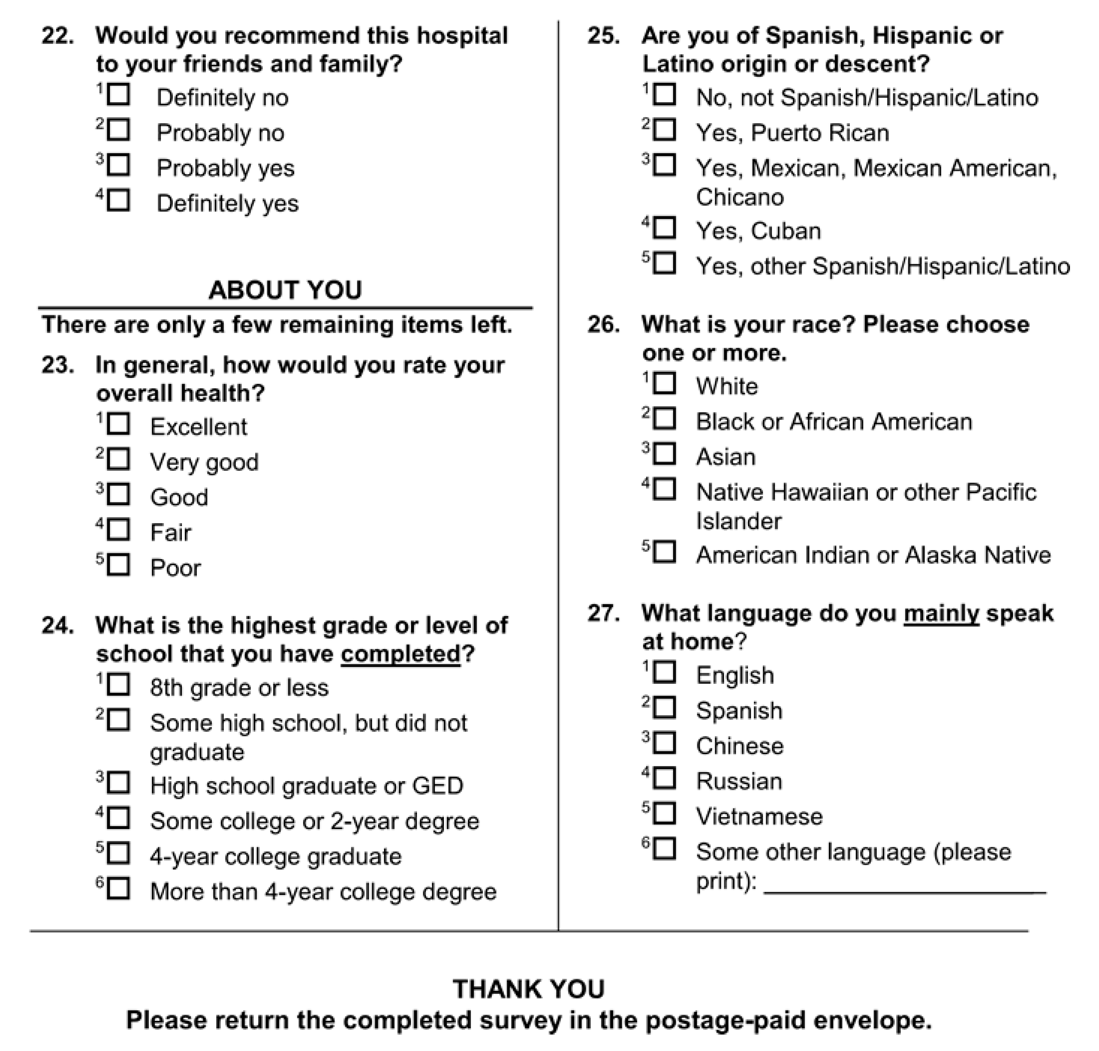
Survey Language	2

presents the types of demographic questions in HCAHPS survey instrument. All demographic identifiers (except for “age” and “discharge date”) are categorical. The HCAHPS survey questionnaire is brought in the Appendix A.

2.2. Review of Existing Studies on HCAHPS Dataset

There have been several studies on the HCAHPS dataset. Stratford [4] defined a number of objectives to extract useful knowledge from the HCAHPS survey data and studied the effect of such knowledge on hospital care improvement.

Sheetz et al. [5] investigated the relationship between postoperative morbidity and mortality and patients’ perspectives of care in surgical patients. In their article, the overall satisfaction score is used along with Michigan Surgical Quality Collaborative clinical registry as a measure of patients’ perspective of care.

Quite a few studies have explored specific relationships between a single satisfaction question and one or more of patients’ demographic information. Goldstein et al. [6] conducted an analysis of racial/ethnicity in patients’ perceptions of inpatient care. Using regression, they concluded that non-Hispanic Whites on average tend to go to hospitals that deliver better patient experiences to all patients as compared to the hospitals that are typically used by African American, Hispanic, Asian/Pacific Islander, or multiracial patients [6].

Elliot et al. analyzed the association of gender with different aspects of satisfaction, [7] and, in a separate study, analyzed hospital ranking variation with patient health status and race/language and slightly with patient’s education and age [8].

Klinkenberg [9] explored the relation between the willingness to recommend the hospital and other satisfaction identifiers. This paper discovers that hospitals that focus resources on improving interpersonal aspects of care such as nurses and doctors’ courtesy, respect, listening, room cleanliness, etc. will be most likely to see improvements in satisfaction scores. The paper does not consider patients’ demographic data.

The existing literature on analysis of the HCAHPS dataset is mostly hypothesis-driven and only considers specific aspects of patient satisfaction or demographics. In contrast, the methodology presented in this paper does not assume any specific hypothesis. Instead, we run a data-driven exploratory analysis which inspects all aspects of patient satisfaction as well as patient demographics and discovers interesting associations in the HCAHPS dataset.

2.3. Shortcomings of Existing Survey Analysis Methods

In addition to the literature on analysis of the HCAHPS dataset; it is also worth reviewing the methods typically used for general survey analysis. Commonly used exploratory data analysis methods such as ANOVA, regression, discriminant analysis, and factor analysis are not applicable to HCAHPS data because of its unique characteristics.

Analysis of variance (ANOVA) is a collection of statistical methods that form an exploratory tool for explaining observations. ANOVA provides a statistical test of whether or not the means of several groups are equal [2]. For finding a specific correlation in the HCAHPS dataset, different levels of ANOVA should be combined. To this end, all possible combinations of satisfaction questions and demographic data should be exhaustively tested, which could be time prohibitive. In addition, ANOVA assumes a normal distribution of the sample observation, continuous dependent variables, and at least one categorical independent variable with two or more levels. The sample data collected for HCAHPS is not guaranteed to be normally distributed. Moreover, the demographic data which form the dependent variables are not always categorical. Given the violation of these assumptions, ANOVA may not produce reliable results for HCAHPS dataset.

Regression analysis is a statistical tool for investigation of relationship between multiple continuous or categorical independent variables and a continuous dependent variable [10]. Regression models can be used for validating correlations, although they are usually used for predicting and forecasting. Variations of this model can be used for the HCAHPS categorical dependent variables and lead to nonlinear models. Using these interpretation, different hypothesis on the data set can be tested by using forward and backward selection of combinations of satisfaction questions and patients’ demographic data. However, forward and backward selection is not efficient in the context of HCAHPS data as the search space contains a very large number of combinations of dependent and independent variables. Moreover, fitting a separate model for each satisfaction identifier cannot capture the relationships between different satisfaction questions.

Discriminant analysis is another technique that allows for studying the difference between two or more groups of objects with respect to several variables simultaneously [11]. This model can be fitted to HCAHPS data set in terms of categorical dependent variables as the satisfaction questions and continuous and categorical independent variables such as patient’s demographical data. Although this method works better than regression in terms of interpreting categorical variables, it suffers from the same deficiencies when it comes to analyzing the HCAHPS dataset.

Factor analysis is another method that is typically applied to survey data. The main application of this method is to reduce the number of variables and to detect structure in the relationship between variables. In particular, factor analysis can be used to explore the data for patterns, confirm hypotheses, or reduce a large number of variables to a more manageable number [12]. Compared to regression and discriminant analysis, factor analysis is more suitable for an exploratory analysis of the HCAHPS dataset as it does not require a priori hypothesis; however, it has two limitations: (1) the naming of the factors can be problematic and may not accurately reflect the variables within that factor. In particular, it may not be possible to directly compile factors into a set of recommendations for the hospitals. (2) factor analysis is based on the assumption that there is a linear relationship between factors and the variables when computing correlations. The features in the HCAHPS survey data may not necessarily be linearly correlated and factor analysis cannot capture non-linear relations.

3. Analyzing HCAHPS Data

This section describes the proposed methodology for analyzing the HCAHPS data. The analysis is done in three steps: 1—data preparation, 2—two-layer cluster analysis, and 3—salient feature extraction and associations.

3.1. Data Preparation

The first problem that should be handled in data preparation is the nature of some questions, called skip questions. A skip question by itself does not provide any information about a patient but it determines whether some other questions, called dependent questions, are applicable to the patient. For instance, a skip question inquires if the patient has used the bathroom or not. If not, the patient skips all of the dependent questions related to the bathroom cleanliness. Since skip questions, by themselves, do not provide any data about a patient, it would be reasonable to omit them from the dataset and treat their empty dependent questions as missing values. For example, if a patient has not used the bathroom, all of the bathroom-related questions have missing value for that patient.

There are two basic approaches for handling missing values: (1) the complete case analysis which ignores the records with missing data, or (2) the imputation of missing values. The imputation method can be further divided into single imputation where each missing value is replaced by a single value, and multiple imputations where each missing value is replaced by multiple values to reflect the uncertainty. The complete case analysis could introduce a selection bias and may lead to loss of information. The added bias makes the data related to those questions more homogenous. If all of the patients have similar opinion on the related questions the added bias will make those questions insignificant. However, if in fact there are two opposite opinions on this matter that are separated based on the demographic features of patients, the separation will be more statistically significant. Therefore, a single imputation method is applied in this study for handling missing values in HCAHPS dataset. This approach may reduce the variance and add bias to range of the imputed variables but will not result in loss of information. The reduction in the variance of an imputed variable may decrease the chance of that variable being selected as a significant feature when compared to other variables, but there is still a chance of being selected if the data is extensively divided on that variable.

For imputing the missing values, the K-nearest neighbor imputation method (KNNI) [13] is used. This method is chosen because it is applicable to both continuous and categorical variables and it can be applied to the data set automatically and without any supervision. This method imputes the missing value based on the K nearest neighbors of the record with missing value. For categorical features, the missing value is replaced with the category which has the majority in the K nearest neighbors. For continuous features, the missing value is replaced with the weighted average of that feature in the nearest neighbors. To have minimum computational complexity, K = 3 has been chosen for KNNI as it is the least number of neighbors that could produce reasonable results for finding majority of classes among categorical variables.

3.2. Two-Layer Cluster Analysis

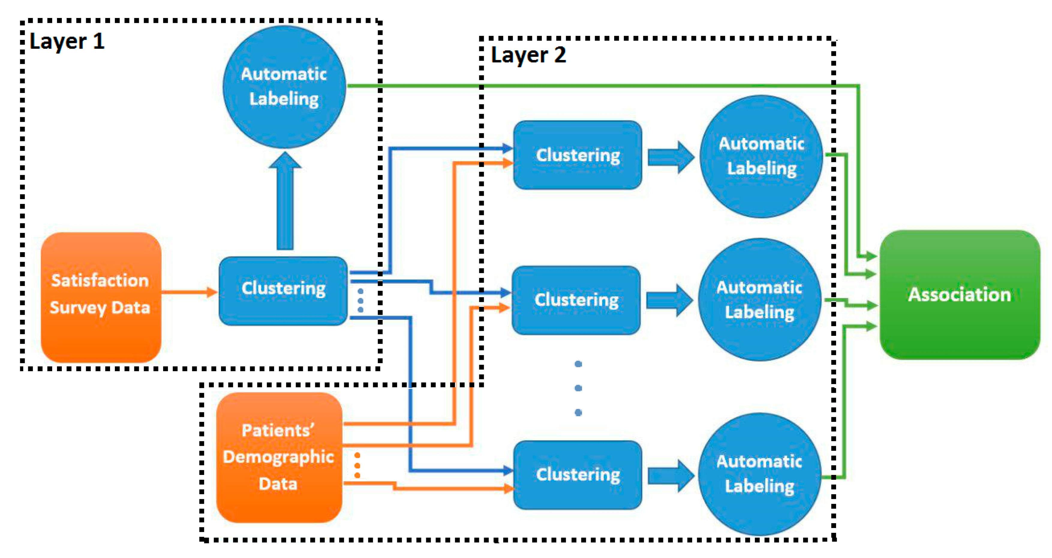
The goal of this step is to do exploratory data analysis in order to find hidden patterns in the HCAHPS dataset and to identify the main sources of patient dissatisfaction. To this end, two layers of clustering is performed on HCAHP data as illustrated in Figure 1.

In the first layer, patient data is clustered based on satisfaction questions (listed in Table 2) to group the patients with similar satisfaction identifiers. We examined various clustering methods such as K-means, DBScan, and Spectral clustering and ultimately decided to choose K-means for its simplicity and efficiency. K-means is the most commonly used clustering method with two main problems. First, it is sensitive to the initialization of the cluster centers and might converge into a local optimum. Second, it requires a pre-specified number of clusters (k). To address the first problem, K-Means++ is typically used to initialize the cluster centroids before proceeding with the standard K-means. With K-means++ initialization, the algorithm is guaranteed to find optimal clusters with $O\left(\log k\right)$ competitive with K-means optimal solution [14]. For solving the second problem, there are several techniques offered to extract the optimal number of clusters. The Calinski-Harabasz criterion method is chosen for the estimation of number of clusters for K-means. This method finds the best number of clusters by applying the criterion of minimum within cluster sum of squares. This procedure ensures an effective reduction of the number of possible splits [15], which prevents overfitting in association extraction procedure. This method is implemented in R using the vegan v2.4-2 package by Jari Oksanen based on the Algorithm 1.

Algorithm 1. Optimal number of clusters using Calinski-Harabasz criterion.

Find Number of Clusters (data, minNumClusters = 1, maxNumClusters = 10 ) Fit ← cascadeKM (data, inf.gr = minNumClusters, sup.gr = maxNumClusters, iter = 100, criterion = “calinski”) calinski_best ← which.max (fit.results [2,]) Return calinski_best

To apply Kmeans++ algorithm on the HCAHPS data with mixed categorical and continuous variables, the categorical variables are transformed to dummy variables and the continuous variables are normalized using z-score normalization. By this transformation all the variables are in one spatial distance range, which is suitable for applying the Kmeans++ algorithm.

After applying Kmeans++ with selected number of clusters, the salient features of each cluster are derived using automatic cluster labeling to mark the important features that make up a cluster. The salient features of a cluster are the ones whose values are significantly different (in a statistical sense) in the cluster compared to those in the other clusters.

The clusters of layer one are then fed into the second layer for further analysis. Each satisfaction cluster of the first layer is clustered again; but this time based on the demographic features of each record listed in Table 2 (e.g., patient’s age, race, etc.). The salient features of each sub-cluster are then derived to find the important features that make up a sub-cluster.

3.3. Salient Feature Extraction

One can draw associations between the salient features of the outer (satisfaction) cluster and the salient features of its inner (demographic) sub-clusters. For instance, suppose that as a result of the first layer we get an outer cluster whose salient features indicate low values for “satisfaction with Doctor”. This cluster is then further clustered into demographic sub-groups. Suppose that the salient features of one of the sub-groups indicates higher values for age and a particular doctor (Doctor X) who visited most patients in this sub-group.

Putting the salient features of a cluster and its sub-clusters together, one can draw an association between older patients who expressed low satisfaction with their doctor and who were visited by Doctor X. Such associations must be further validated through statistical evaluations and can be used to make recommendations to the hospital. For example, the recommendation system might recommend not to assign Doctor X to older patients.

We extract the salient features of each cluster based on the methodology proposed in [16]:

• The centroid of a cluster k is computed as the average of the points in the cluster:

  $$X_k=\frac{{\sum }_{i=1}^N{P}_i}{N}$$

  (1)

  where $X_k$ is the centroid of cluster k and $P_i$ is a point in cluster k.
• The Euclidean distance of each point to its cluster centroid is computed:

  $$d_i=\sqrt{{\displaystyle \sum }_j\left(P_{ij}-X_{kj}\right)}$$

  (2)
• The points in each cluster are divided into in-pattern and out-pattern records. The records whose distance lie within the range defined by (3) are called in-pattern records while all other records including the ones in other clusters are called out-pattern records.

  $${\mu }_k-z{\sigma }_k<d_i<{\mu }_k+z{\sigma }_k$$

  (3)

  where ${\mu }_k$ and ${\sigma }_k$ are the mean and standard deviation of the points in cluster k, respectively, and z is a constant factor. Smaller z results in more out-pattern records and larger z result in more in-pattern records.
• For each feature v and cluster k, the mean of all in-pattern records, ${\mu }_{in}\left(k,v\right)$ and the mean of the out-pattern records, ${\mu }_{in}\left(k,v\right)$, are computed:

  $${\mu }_{in}\left(k,v\right)=\frac{{\sum }_{P_i\in {\phi }_{in}}{P}_{iv}}{\left|{\phi }_{in}\left(k\right)\right|}$$

  (4)

  $${\mu }_{out}\left(k,v\right)=\frac{{\sum }_{P_i\in {\phi }_{out}}{P}_{iv}}{\left|{\phi }_{out}\left(k\right)\right|}$$

  (5)

  where ${\phi }_{in}\left(k\right)$ and ${\phi }_{out}\left(k\right)$ are the set of in-pattern and out-pattern points in cluster k, respectively.
• A difference factor, $df\left(k,v\right)$, is calculated for each feature v in cluster k based on Equation (6):

  $$df\left(k,v\right)=\frac{{\mu }_{in}\left(k,v\right)-{\mu }_{out}\left(k,v\right)}{{\mu }_{out}\left(k,v\right)}$$

  (6)
• The mean and standard deviation of the difference factors for all features in cluster k are calculated as follows:

  $${\mu }_{df}\left(k\right)=\frac{{\sum }_{v-1}^{D}df\left(k,v\right)}{D}$$

  (7)

  $${\sigma }_{df}\left(k\right)=\sqrt{{\displaystyle \sum }_{v-1}^D{\left(df\left(k,v\right)-{\mu }_{df}\left(k\right)\right)}^2/D}$$

  (8)

  where D is the number of features in the input space.
• A feature v is a salient feature in cluster k if its corresponding difference factor in k deviates considerably from ${\mu }_{df}\left(k\right)$. More formally, feature v is a salient feature in cluster k if:

  $$df\left(k,v\right)\le {\mu }_{df}\left(k\right)-z{\sigma }_{df}\left(k\right)$$

  (9)

  $$df\left(k,v\right)\ge {\mu }_{df}\left(k\right)+z{\sigma }_{df}\left(k\right)$$

  (10)

  where z is a constant factor. The smaller the z the more salient features in each cluster. Salient feature extraction method is outlined in Algorithm 2.

Algorithm 2. Salient features extraction.

FindingSalientFeatures (noc, clustered_data, z) Comment: calculating the center of each clustering by averaging records in the cluster.     For i ← 0 to noc − 1         cluster_centers [i] ← average over columns(clustered_data[i]) Comment: calculating distance of records from their assigned cluster center.     For i ← 0 to noc − 1         For j ← 0 to length(clustered_data[i]) − 1             distance_matrix[i][j] ← distance (clustered_data[i][j], cluster_centers [i]) Comment: calculating the average distance of each cluster from its center.     For i ← 0 to noc − 1         average_distance[i] ← average over columns(distance_matrix[i]) Comment: calculating standard deviation of distances in each cluster.     For i ← 0 to noc − 1         standard_deviation[i]←sqrt (average over j((distance_matrix[i][j] − Average_distance[i]) ^2)) Comment: Finding in pattern and out pattern records in each cluster     counter ← 0     For i ← 0 to noc − 1         For j ← to length(clustered_data[i]) − 1             If (distance_matrix[i][j] < (average_distance[i] + (z * standard_deviation[i])) AND distance_matrix[i][j] > (average_distance[i] − (z * standard_deviation[i]))                In_patterns[i][counter] ← j                 counter ++ Comment: Calculating the mean of each feature in each cluster for in-pattern neurons.     For i ← 0 to noc-1         For j ← 0 to length (clustered_data[i]) − 1             If (j in In_patterns[i])                In_pattern_mean[i] ← In_pattern_mean[i] + clustered_data[i]             else                Out_pattern_mean[i] ← Out_pattern_mean[i] + clustered_data[i]        In_pattern_mean[i] ← In_pattern_mean[i]/length(In_patterns[i])        Out_pattern_mean[i] ← Out_pattern_mean[i]/length(Out_patterns[i]) Comment: Calculating the difference factor of in and out pattern records.     For i←0 to noc − 1         For j ← 0 to number_of _columns(clustered_data) − 1             difference_factor [i][j] ← In_pattern_mean[i][j] −             Out_pattern_mean[i][j] Comment: Calculating the mean difference factor of each dimension.     Mean_difference_factor ← average over row(difference_factor) Comment: Calculating the standard deviation difference factor of each cluster.     For i←0 to noc − 1         For j←1 to number_of _columns(clustered_data) − 1             Difference_factor_SD[i] ← Difference_factor_SD[i] +             difference_factor [i][j] − Mean_difference_factor [i])^2)         Difference_factor_SD[i] ← sqrt(Difference_factor_SD[i]/          number_of _columns(clustered_data)) Comment: Calculating a matrix of salient dimentions.     For i ← 0 to noc − 1         For j←  number_of _columns(clustered_data) − 1             If (difference_factor [i][j]<=             (Mean_difference_factor[i] − (z* Difference_factor_SD[i])))                 Salient_dimension[i][j] = −1             else if (difference_factor [i][j]>=             ( Mean_difference_factor[i] + (z* Difference_factor_SD[i])))                 Salient_dimension[i][j] = 1   Return Salient_dimension

To illustrate the extraction of salient features, suppose, as an example, that we have a dataset with five features as shown in

Table 3. Features of Satisfaction Dataset.

Features	Description
D1	Communication with doctor
D2	Communication with Nurse
D3	Pain Management
D4	Cleanliness
D5	Quietness

.

Suppose that the data points of this feature space are clustered into three groups with the centroids listed in

Table 4. Clusters Centroids.

Features	C1	C2	C3
D1	−0.0126243	0.97095961	−0.9913867
D2	0.03791055	−0.07749729	0.02231231
D3	−1.1444478	0.8585494	0.8681821
D4	−1.1509251	0.8681547	0.8681547
D5	−0.00279281	0.009980126	−0.0060900

.

To find the in-pattern and out-pattern records in the cluster, the distances of each record to all three cluster centroids are computed. In addition, the mean and standard deviation of distances for each cluster centroid are calculated. If a record’s distance from a cluster centroid is within one standard deviation from the mean, then it is considered an in-pattern record of that cluster. Otherwise, it is an out-pattern record of the cluster.

Suppose that there are nine records in the dataset.

Table 5. Distance of records from centroid. Bold numbers denote in-pattern records which are in range of one standard deviation from the mean.

Records	C1	C2	C3
R1	1.967133	0.7958750	1.3957300
R2	2.121455	1.6483554	0.9116866
R3	1.675209	1.5959835	1.7050408
R4	1.518996	1.6174912	1.5210744
R5	1.697462	1.0558556	2.1432977
R6	1.843458	0.8124378	1.1173187
R7	1.191784	2.2571117	1.3717867
R8	2.266916	0.7501202	1.4390353
R9	1.706186	1.6242395	1.7090141
R10	1.107229	2.0101626	0.7544890
µ	1.687192	1.367895	1.367732
σ	0.3833892	0.4231975	0.4307547

shows the distance of each record to all three cluster centroids as well as the mean and standard deviation of each cluster. The in-pattern records of each cluster are shown in bold.

After tagging the records in a cluster as in-pattern and out-pattern, the mean of in-pattern records and out-pattern records in each cluster are calculated.

Table 6. Difference Factor of each Feature in each Cluster. Bold numbers are salient features which are out of range of 1 standard deviation from mean.

Features	C1	C2	C3
D1	−0.03037039	1.18199255	−1.22503855
D2	0.04416163	−0.20817361	−0.02380192
D3	−1.537553	1.033197	1.041475
D4	−1.554513	1.045382	1.047448
D5	−0.06825377	−0.03673413	−0.03182003
µ	−0.6293057	0.6031327	0.1616524
Σ	0.7493974	0.5972044	0.8430252

shows the difference factors of each feature in all three clusters along with the mean and standard deviation of the difference factors of each cluster. The salient features are highlighted in bold. For example, D3 (pain management) and D4 (cleanliness of the hospital) are salient features of cluster 1 while D2 (communication with Nurse) and D5 (quietness) are salient features of cluster 2. The positive values of significant difference factors show high frequency of dichotomous variables and high values for other categorical and continuous variables. Similarly, negative values show a low frequency for dichotomous variables and low values for other categorical and continuous variables. For instance, D3 (pain management) has negative difference factor for cluster one which shows low values of this variable, so the satisfaction with pain management is generally low in this cluster. Similarly, a high satisfaction with pain management can be inferred from cluster three. The salient features of each cluster are presented in

Table 7. Salient features.

Cluster	Salient Features
C1	Pain Management	Low
	Cleanliness	Low
C2	Communication with Nurse	Low
	Quietness	Low
C3	Communication with doctor	Low
	Pain Management	High
	Cleanliness	High

, along with the range of that value or frequency of dichotomous value (High/Low) next to each of them. The salient features with the range of their values are a representation of the cluster, which will be used to create associations.

4. Experiment

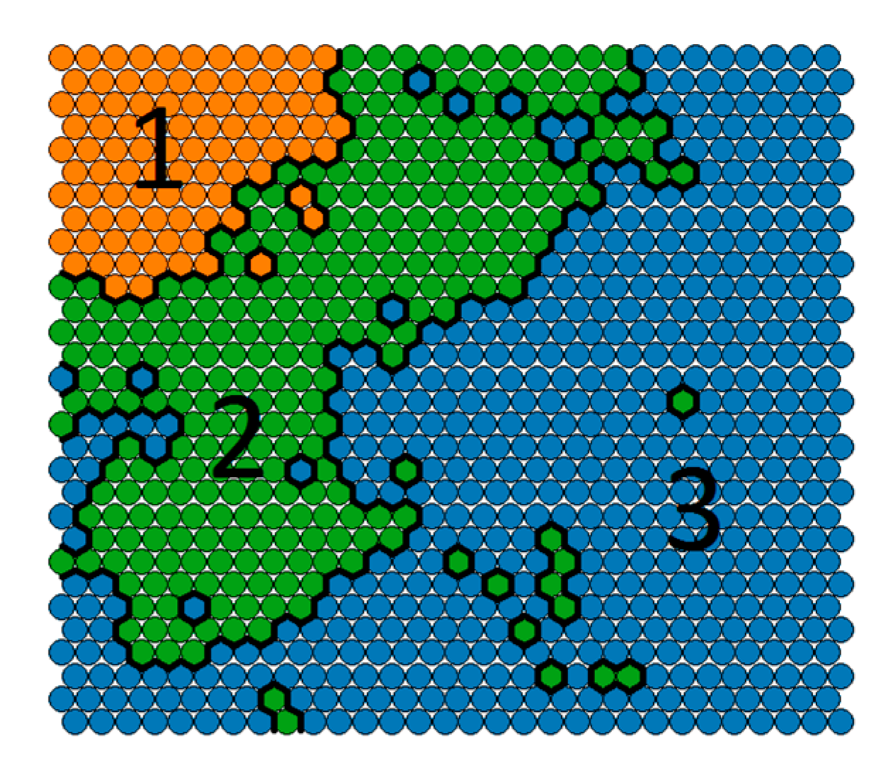
The methodology proposed in the previous section is implemented in R and is applied to the HCAHPS dataset of a hospital with 2652 records with the same features explained in Section 2.1. First, K-means++ is used to cluster all records based on the patients’ responses to the satisfaction questions. A Self-organizing feature map is used to visualize data distribution in each cluster (Figure 2).

The map shows that Kmeans++ divided data according to the Calinski-Harabasz [15] criterion into three clusters based on their responses to the satisfaction questions. These clusters are shown in different colors in Figure 2. In the next step, the salient features of each cluster are extracted to identify the most important features which constitute a cluster. Extracted salient features were interpreted according to nature of each variable whether it is continuing, categorical, or dichotomous.

Table 8. Salient features of clusters in the first layer.

Cluster	Salient Features
C1	High Satisfaction with Help after discharge High Satisfaction with Symptoms info High Overall Health
C2	High Satisfaction with Help after discharge High Satisfaction with Symptoms info
C3	Low Satisfaction with Help after discharge Low Satisfaction with Symptoms info Low Overall Health

asserts the interpretation of the extracted salient features. For example, cluster 1 represent patients who were well-informed about their symptoms after leaving the hospital and expressed high satisfaction with help after discharge and high overall satisfaction.

Although theoretically salient features are expected be different in different clusters, this expectation could be violated if the clusters are of significantly different sizes. For example, in Table 2, C1, and C2 share some features (i.e., high satisfaction with help after discharge and high satisfaction with symptoms info). This is due to the fact that C3 is much bigger than C1 and C2 (Figure 1). Therefore, it has a significant effect on the value of difference factor, highlighting the shared salient features in C1 and C2. Although it might appear that C2 is redundant, C1 and C2 were divided into two distinct clusters mainly because of their difference in the overall health feature.

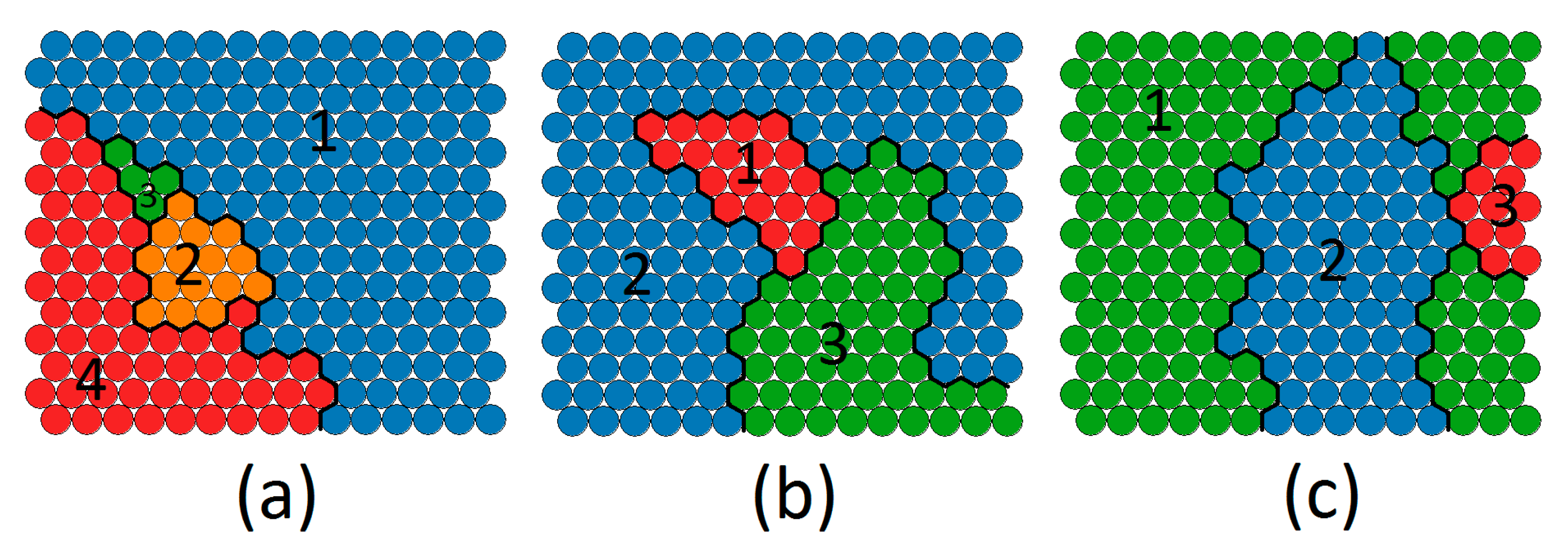
The records in each cluster are fed into the second layer of clustering. In this layer, patients are clustered based on their demographic data such as (e.g., age, sex, race, etc.). The first cluster is divided into four demographic sub-clusters and the second and third clusters are both divided into three demographic sub-clusters. The process is outlined in Algorithm 3 and the outcome of this step is visualized in Figure 3.

Algorithm 3. Recommendation extraction.

Find Recommendations (data, split_index)     Satisfaction_questions_data ← data [:] [0:split_index]     noc ← FindNumberOfClusters (Satisfaction_questions_data )     Sq_clustered_data = kmeans (Satisfaction_questions_data)     Sq_salient_dim ← FindingSalientFeatures (noc, Sq_clustered_data, z)     For i ← 0 to noc         For j in Sq_clustered_data[i]             Demographic_data ← data[j] [split_index: number_of_columns(data)]             D_clustered_data ← kmeans (Demographic_data)             D_salient_dim ← FindingSalientFeatures (noc, D_clustered_data, z)         For sq_salient in Sq_salient_dim[i]:             If sq_salient != 0:                 For d_salient in D_salient_dim:                     If d_salient != 0:                       Recommendation                     [(col_name(sq_salient), sq_salient)].                      Add ((col_name(d_salient), d_salient))   Return recommendation

Once again salient feature extraction algorithm is applied on each sub-cluster. The results are asserted in

Table 9. Salient features of all satisfaction clusters and their demographic sub-clusters (Numbers in parenthesis demonstrate the clusters’ populations).

Cluster	C1 (1210 Observations)
Cluster Salient Features	High Satisfaction with Help after discharge High Satisfaction with Symptoms info High Overall Health
Sub-cluster	SC1 (378 obs.)	SC2 (236 obs.)	SC3 (268 obs.)	SC4 (328)
Sub-cluster Salient Features	Mostly not Spanish/Hispanic/Latino Ethnicity Mostly Spanish Language	Mostly Old Mostly Emergency Room Admission Source Mostly Medical Principal Reason of Admission	Mostly Young Mostly Female Mostly Physician Referral Admission Source Mostly Obstetric Principal Reason of Admission	Mostly Old Mostly Physician Referral Admission Source Mostly Surgical Principal Reason of Admission
Cluster	C2 (602 Observations)
Cluster Salient Features	High Satisfaction with Help after discharge High Satisfaction with Symptoms info
Sub-cluster	SC1 (141 obs.)	SC2 (224 obs.)	SC3 (237 obs.)
Sub-cluster Salient Features	Mostly Old Mostly Emergency Room Admission Source Mostly Medical Principal Reason of Admission	Mostly Physician Referral Admission Source Rarely Medical Principal Reason of Admission	Rarely not Spanish/Hispanic/Latino Ethnicity Mostly Spanish Language
Cluster	C3 (840 Observations)
Cluster Salient Features	Low Satisfaction with Help after discharge Low Satisfaction with Symptoms info Low Overall Health
Sub-cluster	SC1 (278 obs.)	SC2 (296 obs.)	SC3 (266 obs.)
Sub-cluster Salient Features	Mostly Old Mostly Emergency Room Admission Source Mostly Medical Principal Reason of Admission	Rarely not Spanish/Hispanic/Latino Ethnicity Mostly Spanish Language	Mostly Physician Referral Admission Source Mostly Obstetric Principal Reason of Admission

.

Putting the salient features of a satisfaction cluster and the salient features of its demographic sub-cluster, we derived the associations listed in

Table 10. Derived Associations.

1	Patients who have high Satisfaction with Help After Discharge, have these qualities: Mostly Physician Referral Admission Source, Mostly not Medical Principal Reason of Admission
2	Patients who have high Satisfaction with Symptoms Info, have these qualities: Mostly Physician Referral Admission Source, Rarely Medical Principal Reason of Admission
3	Patients who have high Satisfaction with Help After Discharge, have these qualities: Rarely White Race
4	Patients who have high Satisfaction with Symptoms Info, have these qualities: Rarely White Race
5	Patients who have high Satisfaction with Help After Discharge, have these qualities: Mostly Old, Mostly Emergency Room Admission Source, Mostly Medical Principal Reason of Admission
6	Patients who have high Satisfaction with Symptoms Info, have these qualities: Mostly Old, Mostly Emergency Room Admission Source, Mostly Medical Principal Reason of Admission
7	Patients who have low Satisfaction with Help After Discharge, have these qualities: Mostly Old, Mostly Physician Referral Admission Source, Mostly Surgical Principal Reason of Admission
8	Patients who have low Satisfaction with Symptoms Info, have these qualities: Mostly Old, Mostly Physician Referral Admission Source, Mostly Surgical Principal Reason of Admission
9	Patients who have low Satisfaction with Help After Discharge, have these qualities: Mostly Young, Mostly Female, Mostly Physician Referral Admission Source, Mostly Obstetric Principal Reason of Admission
10	Patients who have low Satisfaction with Symptoms Info, have these qualities: Mostly Young, Mostly Female, Mostly Physician Referral Admission Source, Mostly Obstetric Principal Reason of Admission
11	Patients who have low Satisfaction with Help After Discharge, have these qualities: Mostly Old, Mostly Emergency Room Admission Source, Mostly Medical Principal Reason of Admission
12	Patients who have low Satisfaction with Symptoms Info, have these qualities: Mostly Old, Mostly Emergency Room Admission Source, Mostly Medical Principal Reason of Admission
13	Patients who have high Satisfaction with Help After Discharge, have these qualities: Mostly Physician Referral Admission Source, Mostly Obstetric Principal Reason of Admission
14	Patients who have high Satisfaction with Symptoms Info, have these qualities: Mostly Physician Referral Admission Source, Mostly Obstetric Principal Reason of Admission
15	Patients who have high Satisfaction with Help After Discharge, have these qualities: Rarely not Spanish/Hispanic/Latino Ethnicity, Rarely English Language
16	Patients who have high Satisfaction with Help After Discharge, have these qualities: Rarely not Spanish/Hispanic/Latino Ethnicity, Rarely English Language
17	Patients who have high Satisfaction with Help After Discharge, have these qualities: Mostly Old, Mostly Emergency Room Admission Source
18	Patients who have high Satisfaction with Symptoms Info, have these qualities: Mostly Old, Mostly Emergency Room Admission Source
19	Patients who have high Overall health, have these qualities: Mostly Old, Mostly Emergency Room Admission Source

. These associations represent a possible source of significant satisfaction questions. For instance, the source of low satisfaction with help after discharge according to C3 is communication with old people referred from a physician or Spanish speaking patients admitted from the emergency room. Transforming these associations into recommendations can offer hospital policy changes in favor of both patients and hospitals. The proper recommendation in this case can be putting more effort in communication with elderly people and Spanish people, or hiring a Spanish speaking nurse or interpreter.

It is worth noting, that the method explained in this section, works better in terms of performance and accuracy than in methods such as association rule mining, which has its well-known limitations including a brute-force method for extracting association rules and the risk of finding many irrelevant rules.

5. Validation

The associations derived from the two-layer clustering must be validated through standard statistical tests to ensure that they did not occur by chance. This is a very important step for generating reliable associations. Each of the associations is considered as a hypothesis and it is tested based on the whole data set. As described, almost all of the features in the data set are categorical or even dichotomous, which are of multiple groups of studies with unequal sample sizes. In order to work with such data, chi-square test of independence is used for hypothesis testing.

The Chi-square statistic is a non-parametric tool designed to analyze group differences when the dependent variable is measured at a nominal level [17]. This test is robust to the distribution of data. The null hypothesis is stated as H0: the two classifications are independent, while the alternative hypothesis is H1: the classifications are dependent. The significance of the test is calculated according to the frequency contingency table of the independent classes (Each item in data set belongs only to one class). This value is compared with the critical values in the chi-square table, and if it is larger than this critical value, then the null hypothesis is rejected. Typically, if the chi-square test p-value is lower than 0.05, the independence of the features in the association is rejected.

Before using chi-square test for validating the associations, we have to make sure that the dataset meets the assumptions of the chi-square. The chi-square test requires that no more than 20% of the frequencies of categories are less than five; otherwise the calculated p-values may not be accurate. There are many empty or low frequency categories in the patients’ contingency table that consists of more than 35% of the frequencies. By combining the columns or rows this issue can be resolved. For example,

Table 11. Contingency Table for Satisfaction with Symptoms Info and rarely not Spanish/Hispanic/ Latino and Spanish Language.

Satisfaction with Symptoms Info	Rarely Not Spanish/Hispanic/Latino Ethnicity Spanish Language
	0.0	1.0	0.1	1.1
1	3	180	1710	249
2	1	32	521	63
3	0	6	94	7
4	0	5	72	5

illustrates a 3-way contingency table for testing the 16 association in Table 10. The rows are the satisfaction of symptoms info and the columns are a combination of not Spanish, Hispanic or Latino and the Spanish language. The two-digit binary values in the first row indicate a combination of not Spanish, Hispanic, or Latino Ethnicity (Yes/No) and Spanish Language (Yes/No). For example, 0.0 in the first row indicates that the patients are rarely not Spanish, Hispanic or Latino Ethnicity, and they speak Spanish. In order to get higher frequencies, we can combine the first two rows into a single row to indicate a “low” satisfaction. Similarly, we can merge the last two rows to indicate a “high” satisfaction (

Table 12. Contingency Table with Combined Rows.

Satisfaction with Symptoms Info	Rarely Not Spanish/Hispanic/Latino Ethnicity Spanish Language
	0.0	1.0	0.1	1.1
Low	4	212	2231	256
High	0	11	166	12

). The rows must be combined in a way to yield an interpretable result. The algorithm proposed for this modification to chi-square test is delineated in Algorithm 4.

Algorithm 4. Modified chi-square test.

Modified_chisquare(interaction_table):     Comment: Adjusting interaction table not to have values less than five.     Col ← 0 to num_col(interaction_table):     If all(table[, col] < 5):         table1 ← table [, -col]         table ← table1         col ← col−1         numcol ← numcol−1    col ← col + 1    return chisq.test(table)

The frequencies can further be improved by combining the first two columns as shown in

Table 13. Contingency with combined Rows and Columns.

Satisfaction with Symptoms Info	Rarely Not Spanish/Hispanic/Latino Ethnicity Spanish Language
	X.0	0.1	1.1
Low	216	2231	256
High	11	166	12

.

The interpretation of the contingency table needs to be done carefully when combining the rows or columns. For example, Table 13 indicates that 216 non-Spanish speaking patients were not satisfied with information provided about their symptoms after discharge. The process of combining the rows and columns continuous until the resulting frequencies satisfy the Chi-square test assumptions.

The chi-square test can be used to prove the validity of an association but it does not give any measure to assess the strength of each valid association. After filtering out the invalid associations using chi-square test, we use odds ratio [18] to measure the strength of each association and to rank them based on their strength. Odds ratio is a measure of association between a condition and an outcome. The odds ratio shows the odds that an outcome will occur in a particular condition, as compared to the odds of the outcome occurring in other conditions. A z-test is used to compare two odds ratios. The significance of the z-test is measured by its p-value. If the p-value is bigger than 2 or smaller than −2, then the association is considered significant both in terms of dependency and strength. Odds ratio is not dependent to the sample size and it can provide a basis to compare the strengths of the associations extracted from the two-layer clustering between patients’ satisfaction identifiers and their demographics. Using these two-step validations, recommendations created because of noise in the data are removed, which alleviates the overfitting that could have happened in the process.

Most associations extracted from the patient dataset have more than two features. Before computing the odds ratio, the contingency table should be converted to a two by two table. The converted table is made by calculating the frequencies of instances that meet the demographic conditions in the derived association and the ones that don’t meet these conditions.

Table 14. Two by Two Table.

Satisfaction with Symptoms Info	Condition: Rarely Not Spanish/Hispanic/Latino Ethnicity High Spanish Language
	Meet Condition	Do Not Meet Conditions
Low	2447	256
High	177	12

converts the contingency table in Table 13 to a two by two table for calculating the odds ratio.

Having converted the contingency table to a two by two table, the odds ratio of each cell in the table is calculated. A z-test is used to compare the odds ratio of the patients meeting the conditions versus the ones who do not having the same satisfaction level. The significance of the z-test is measured by its p-value. If the absolute p-value is greater than 2, then the association is considered significant both in terms of dependency and strength. Unlike chi-square test, the p-value of the z-test can be used both for omitting weak, irrelevant associations and for ranking them. This pseudo code for the validation function used is depicted in Algorithm 5.

Algorithm 5. Validation function.

validate_relationships (recommendation)     Interaction_table ← interact(recommendation)     Chisqr ← Modifies_chisquare(Interaction_table)     If Chisqr. P_value < 0.5:         For row in interaction_table.rows:             For col in interaction_table.cols:                 Odds_ratio ← Odds_ratio(interaction_table,row,col)                     If odds_ratio.p_value > 2 or odds_ratio.p_value < −2:                         Return True       Return False

Table 15. Validation results of extracted associations from the HCAHPS data related to one hospital.(Linked to Table 10 by row number). Bold figures are p-values in accepted test ranges.

1	Chi-square	X-squared = 28.104	p-value = 3.455 × 10−6
	z-test	p-value = 5.00891912614554
2	Chi-square	X-squared = 7.084	p-value = 0.06927
	z-test	p-value = 0.0183582852328812
3	Chi-square	X-squared = 1.5969	p-value = 0.2063
	z-test	p-value = 1.31385601104743
4	Chi-square	X-squared = 0.50012	p-value = 0.4794
	z-test	p-value = −0.760696016958917
5	Chi-square	X-squared = 30.14	p-value = 0.001506
	z-test	p-value = −2.9118314808416
6	Chi-square	X-squared = 43.594	p-value = 8.558 × 10−6
	z-test	p-value = −0.212828628801027
7	Chi-square	X-squared = 26.86	p-value = 0.004825
	z-test	p-value = −1.97247635563556
8	Chi-square	X-squared = 63.926	p-value = 1.715 × 10−9
	z-test	p-value = 3.59338301942709
9	Chi-square	X-squared = 25.48	p-value = 0.01271
	z-test	p-value = −3.39514132553282
10	Chi-square	X-squared = 61.28	p-value = 1.315 × 10−8
	z-test	p-value = −5.48685043800752
11	Chi-square	X-squared = 30.14	p-value = 0.001506
	z-test	p-value = 2.9118314808416
12	Chi-square	X-squared = 43.594	p-value = 8.558 × 10−6
	z-test	p-value = 0.212828628801027
13	Chi-square	X-squared = 20.061	p-value = 0.0001649
	z-test	p-value = 3.50130627065847
14	Chi-square	X-squared = 43.489	p-value = 1.937 × 10−9
	z-test	p-value = 5.57545804293131
15	Chi-square	X-squared = 8.8791	p-value = 0.03094
	z-test	p-value = 2.45951143035353
16	Chi-square	X-squared = 0.9116	p-value = 0.8226
	z-test	p-value = −0.774093020800148
17	Chi-square	X-squared = 18.715	p-value = 0.002172
	z-test	p-value = −2.85471982135127
18	Chi-square	X-squared = 27.572	p-value = 4.413 × 10−5
	z-test	p-value = −1.47076729692434
19	Chi-square	X-squared = 24.691	p-value = 0.0001599
	z-test	p-value = −0.231962167837976

lists the p-values of the chi-square and the z-tests for each association derived in Table 10. Associations with significant values are shown in bold figures. If both p-values values are significant, than the association is considered accurate and reliable. Otherwise, the association is omitted as there is not enough evidence to support its significance. The list of cleaned associations is ranked based on the p-value of z-test and presented in

Table 16. The list of cleaned associations ranked based on their odds ratio.

1	Patients who have high Satisfaction with Symptoms Info, have these qualities: Mostly Physician Referral Admission Source, Mostly Obstetric Principal Reason of Admission
	z-test	p-value = 5.57545804293131
2	Patients who have low Satisfaction with Symptoms Info, have these qualities: Mostly Young, Mostly Female, Mostly Physician Referral Admission Source, Mostly Obstetric Principal Reason of Admission
	z-test	p-value = −5.48685043800752
3	Patients who have high Satisfaction with Help After Discharge, have these qualities: Mostly Physician Referral Admission Source, Rarely Medical Principal Reason of Admission
	z-test	p-value = 5.00891912614554
4	Patients who have low Satisfaction with Symptoms Info, have these qualities: Mostly Old, Mostly Physician Referral Admission Source, Mostly Surgical Principal Reason of Admission
	z-test	p-value = 3.59338301942709
5	Patients who have high Satisfaction with Help After Discharge, have these qualities: Mostly Physician Referral Admission Source, Mostly Obstetric Principal Reason of Admission
	z-test	p-value = 3.50130627065847
6	Patients who have low Satisfaction with Help After Discharge, have these qualities: Mostly Young, Mostly Female, Mostly Physician Referral Admission Source, Mostly Obstetric Principal Reason of Admission
	z-test	p-value = −3.39514132553282
7	Patients who have high Satisfaction with Help After Discharge, have these qualities: Mostly Old, Mostly Emergency Room Admission Source, Mostly Medical Principal Reason of Admission
	z-test	p-value = −2.9118314808416
8	Patients who have high Satisfaction with Help After Discharge, have these qualities: Mostly Old, Mostly Emergency Room Admission Source
	z-test	p-value = −2.85471982135127
9	Patients who have high Satisfaction with Help After Discharge, have these qualities: Rarely not Spanish/Hispanic/Latino Ethnicity, Rarely English Language
	z-test	p-value = 2.45951143035353
10	Patients who have high Satisfaction with Symptoms Info, have these qualities: Mostly Old, Mostly Emergency Room Admission Source, Mostly Medical Principal Reason of Admission
	z-test	p-value = −0.212828628801027

.

6. Turning Associations into Recommendations for Hospitals

The associations extracted in the previous section can be used in two ways to improve patient experience for various patient groups:

• The valid association can be simply transformed into a set of general applicable recommendations. For instance, based on the second association in Table 16, the system can make the recommendation that “Young ladies whose admission source is physician referral and their reason of admission is obstetrical, need more information about their symptoms when they are being discharged”. In this approach, one recommendation is generated for each correlation, although, the recommendations which are based on patients’ dissatisfaction are probably more useful than ones which are based on patients’ satisfaction.
• The associations can be used to produce target-based recommendations. Assume that a patient is being admitted to a hospital. The reception takes the patient’s information and relative recommendations would be popped out. For instance, suppose an old patient with physician referral is being admitted for surgical reason. Based on the 4th correlation in Table 4, a recommendation is shown to the health care provider asserting that this patient needs more information about her/his symptoms. This can be accomplished by a simple rule-based expert system.

7. Conclusions

In this work, an unsupervised exploratory data analysis methodology is introduced to discover associations between patients’ demographics and their various satisfaction identifiers. Such associations are extracted using a two-layer cluster analysis together with extracting the salient features of each cluster. The associations are validated using statistical tests and are ranked based on their significance. The goal was to use such associations to create a patient satisfaction based the recommendation system for hospitals. The methodology was applied to HCAHP data obtained from CAHPS Database and the generated recommendations were validated using statistical tests. In the presented case study in this work, the proposed methodology, extracted nineteen associations from the HCAHPS dataset of a hospital with 2652 records. Ten associations out of nineteen were validated through statistical methods of chi-squared independence test, and odds ratio z-test, which shows the reliability of the proposed recommendation system.

The proposed recommendation system provides knowledge that may be hidden to an expert analyzing the surveys and rectifies the need for a subject-matter expert. The analysis approach is designed specifically for the format of the standard HCAHPS survey; however, it can be extended to other domains in which customer survey plays an important role.

The future work of this study will focus on three aspects:

• More extensive data collection: Our long-term goal is to assess how the recommendations produced by our system can improve patients’ loyalty and result in saving costs and time in the long run. Using the preliminary results outlined in this paper, our goal is to obtain a more comprehensive data set which includes data on whether the patients have come back to the hospital if medical services were needed, and to examine the relationship between customer loyalty and their satisfaction identifiers.
• Handling skip questions: In this study, a single imputation method based on K-nearest neighbor (KNN) is used to impute missing values. Other popular approaches, such as multiple imputations by chained equations (MICE) [19], should be explored in future for imputing both categorical and continues variables. Also, other approaches for handling skip questions should be examined to better distinguish between non-applicable and missing data.
• Alternative distance measures for K-means: In this study, we used Euclidean distance for clustering. Euclidean distance is typically used for continuous data where data are seen as points in the Euclidean space. Since HCAHPS data consist of mixed numeric and categorical variables, we should examine other types of distance measures such as cosine, Jaccard, Overlap, Occurrence Frequency, etc. [20] and compare the quality of recommendations produced by each measure. In addition, since there are two layers of clustering and the intrinsic characteristics of data points in each layer vary, and a different distance function can be used for each layer.

References

- Lehtonen, R.; Pahkinen, E. Practical Methods for Design and Analysis of Complex Surveys; John Wiley & Sons: Hoboken, NJ, USA, 2004. [Google Scholar]
- Kenett, R.; Salini, S. Modern Analysis of Customer Surveys: With Applications Using R (Vol. 117); John Wiley & Sons: Hoboken, NJ, USA, 2011. [Google Scholar]
- Giordano, L.A.; Elliott, M.N.; Goldstein, E.; Lehrman, W.G.; Spencer, P.A. Development, implementation, and public reporting of the HCAHPS survey. Med. Care Res. Rev. 2010, 67, 27–37. [Google Scholar] [CrossRef] [PubMed]
- Stratford, N.J. Patient perception of pain care in the United States: A 5-year comparative analysis of hospital consumer assessment of health care providers and systems. Pain Phys. 2014, 17, 369–377. [Google Scholar]
- Sheetz, K.H.; Seth, A.W.; Micah, E.G.; Darrell, A.C., Jr.; Michael, J.E. Patients’ perspectives of care and surgical outcomes in Michigan: an analysis using the CAHPS hospital survey. Ann. Surg. 2014, 260, 5–9. [Google Scholar] [CrossRef] [PubMed]
- Goldstein, E.; Marc, N.E.; William, G.L.; Katrin, H.; Laura, A.G. Racial/ethnic differences in patients’ perceptions of inpatient care using the HCAHPS survey. Med. Care Res. Rev. 2010, 67, 74–92. [Google Scholar] [CrossRef] [PubMed]
- Elliott, M.N.; William, G.L.; Megan, K.B.; Elizabeth, G.; Katrin, H.; Laura, A.G. Gender differences in patients’ perceptions of inpatient care. Health Serv. Res. 2012, 47, 1482–1501. [Google Scholar] [CrossRef] [PubMed]
- Elliott, M.N.; William, G.L.; Elizabeth, G.; Katrin, H.; Megan, K.B.; Laura, A.G. Do hospitals rank differently on HCAHPS for different patient subgroups? Med. Care Res. Rev. 2010, 67, 56–73. [Google Scholar] [CrossRef] [PubMed]
- Klinkenberg, W.; Dean, S.B.; Brian, M.W.; Koichiro, O.; Joe, M.I.; Jan, C.G.; Wm Claiborne, D. Inpatients’ willingness to recommend: a multilevel analysis. Health Care Manag. Rev. 2011, 36, 349–358. [Google Scholar] [CrossRef] [PubMed]
- Kleinbaum, D.; Lawrence, K.; Azhar, N.; Eli, R. Applied Regression Analysis and Other Multivariable Methods; Nelson Education: Scarborough, ON, Canada, 2013. [Google Scholar]
- Scholkopft, B.; Klaus-Robert, M. Fisher Discriminant Analysis with Kernels. In Proceedings of the Neural Networks for Signal Processing IX, Madison, WI, USA, 25 August 1999. [Google Scholar]
- Thurstone, L.L. Multiple factor analysis. Psychol. Rev. 1931, 38, 406. [Google Scholar] [CrossRef]
- Batista, G.E.; Monard, M.C. A Study of K-Nearest Neighbour as an Imputation Method. HIS 2002, 87, 251–260. [Google Scholar]
- Ailon, N.; Ragesh, J.; Claire, M. Streaming k-means approximation. In Advances in Neural Information Processing Systems; Columbia University: New York, NY, USA, 2009; pp. 10–18. [Google Scholar]
- Caliński, T.; Jerzy, H. A dendrite method for cluster analysis. Commun. Stat.-Theory Methods 1974, 3, 1–27. [Google Scholar] [CrossRef]
- Azcarraga, A.P.; Hsieh, M.H.; Pan, S.L.; Setiono, R. Extracting salient dimensions for automatic SOM labeling. IEEE Trans. Syst. Man Cybern. Part C 2005, 35, 595–600. [Google Scholar] [CrossRef]
- McHugh, M.L. The chi-square test of independence. Biochem. Med. 2013, 23, 143–149. [Google Scholar] [CrossRef]
- Bland, J.M.; Douglas, G.A. The odds ratio. BMJ 2000, 320, 1468. [Google Scholar] [CrossRef] [PubMed]
- White, I.R.; Patrick, R.; Angela, M.W. Multiple imputation using chained equations: Issues and guidance for practice. Stat. Med. 2011, 30, 377–399. [Google Scholar] [CrossRef] [PubMed]
- Boriah, S.; Varun, C.; Vipin, K. Similarity measures for categorical data: A comparative evaluation. In Proceedings of the 2008 Society for Industrial and Applied Mathematics (SIAM) International Conference on Data Mining, Atlanta, GA, USA, 24–26 April 2008; pp. 243–254. [Google Scholar]
Figure 1.
Two-layered analysis method. In the first layer, the clusters and their labels are generated based on the satisfaction questions. In second layer, the clusters of first layer are re-clustered based on patient demographic data.
Figure 2.
The clusters produced based on patients’ responses to satisfaction questions.
Figure 3.
Sub-clusters produced based on patient demographic data (a) demographic sub-clusters of the first satisfaction cluster, (b)demographic sub-clusters of the second satisfaction cluster, (c) demographic subclusters of the third satisfaction cluster.